MBIS: Multivariate Bayesian Image Segmentation Tool

Abstract

We present MBIS (Multivariate Bayesian Image Segmentation tool), a clustering tool based on the mixture of multivariate normal distributions model. MBIS supports multichannel bias field correction based on a B-spline model. A second methodological novelty is the inclusion of graph-cuts optimization for the stationary anisotropic hidden Markov random field model. Along with MBIS, we release an evaluation framework that contains three different experiments on multi-site data. We first validate the accuracy of segmentation and the estimated bias field for each channel. MBIS outperforms a widely used segmentation tool in a cross-comparison evaluation. The second experiment demonstrates the robustness of results on atlas-free segmentation of two image sets from scan-rescan protocols on 21 healthy subjects. Multivariate segmentation is more replicable than the monospectral counterpart on T1-weighted images. Finally, we provide a third experiment to illustrate how MBIS can be used in a large-scale study of tissue volume change with increasing age in 584 healthy subjects. This last result is meaningful as multivariate segmentation performs robustly without the need for prior knowledge.

1 Introduction

Brain tissue segmentation from magnetic resonance imaging (MRI) has been one of the most challenging problems in computer vision applied to biomedical image analysis [kapur_segmentation_1996]. It is intended to provide precise delineations of white matter (WM), gray matter (GM) and cerebrospinal fluid (CSF) from acquired data. Brain tissue segmentation is the standpoint of processing schemes in an endless number of research studies concerning brain morphology, such as quantitative analyses of tissue volumes [mortamet_effects_2005, abe_sex_2010, taki_correlations_2011], studies of cortical thickness [fischl_measuring_2000, jones_three-dimensional_2000, macdonald_automated_2000], and voxel-based morphometry [wright_voxel-based_1995, paus_structural_1999, good_voxel-based_2001, ge_age-related_2002]. In a clinical context, numerous studies have demonstrated the potential use of brain tissue segmentation. The spatial location of the above key anatomical structures within the brain is a requirement for clinical intervention [kikinis_digital_1996] (e.g. radiotherapy planning, surgical planning, and image-guided intervention). Early applications addressed global conditions; for example [tanabe_tissue_1997] used semiautomated segmentation of MRI to assess the decrease in total brain tissue and cortical GM, and ventricle enlargement in Alzheimer’s Disease patients. Another study [hazlett_cortical_2006] presented an automated methodology to identify abnormal increase of the GM volume in individuals with autism. Focal conditions have also been studied, including extra classes in clustering and some other adaptations of methods to pathologies, such as automated tumor delineation [prastawa_automatic_2003], lesion detection and volume analyses in multiple sclerosis [collins_automated_2001, zijdenbos_automatic_1998, zijdenbos_automatic_2002, van_leemput_automated_2001, van_leemput_unifying_2003], and white matter lesions associated with age and several conditions like clinically silent stroke, and higher systolic blood pressure [anbeek_probabilistic_2004]. The accurate and automated segmentation of tumor and edema in multivariate brain images is an active field of interest in medical image analysis, as illustrated by the Challenge on Multimodal Brain Tumor Segmentation [menze_multimodal_2014] that has been held in conjunction with the last three sessions of the Medical Image Computing and Computer Assisted Intervention (MICCAI) International Conference.

A survey on brain tissue segmentation techniques is reported elsewhere [liew_current_2006]. Currently popular methodologies can be grouped into three main families. Deformable model fitting approaches [suri_leaking_2000, yushkevich_user-guided_2006, roura_marga:_2012, delibasis_novel_2013, dang_validation_2013] are designed to evolve a number of initial contours towards the intensity steps that occur at tissue interfaces. Atlas-based methods [gorthi_active_2011] use image registration to perform a spatial mapping between the actual data and an anatomical reference called an atlas. The atlas is prior knowledge on the morphology of data, and it generally comprehends a partition previously extracted by any other means (i.e. manual delineation, averaging large populations, etc.). Clustering or classification algorithms [van_leemput_automated_1999-1, ahmed_modified_2002, vrooman_multi-spectral_2007, ji_generalized_2012] search for a pixel-wise partition of the image data into a certain number of categories or clusters (i.e. WM, GM, and CSF). The partition can be hard when each pixel belongs to a single cluster or fuzzy, assigning a probability of membership to each category, which yields a so-called tissue probability map (TPM) per class. These three families of segmentation strategies have often been combined to obtain enhanced results. For instance, deformable models can be initialized using contours already located close to the solution sought using atlases. In clustering methods, priors usually take the form of precomputed TPMs derived from the atlas. These prior probability maps can be used just to initialize the model, or be integrated throughout the model fitting process [ashburner_unified_2005], simultaneously improving the atlas registration at each iteration. The use of priors presents two particular properties. On one hand, it generally aids the segmentation process providing great stability and robustness. However, it is also suspected to bias results, driving the solution somewhat close to the population features that underlie the atlas [davatzikos_why_2004]. One further concern about the use of priors is posed by the need for a spatial mapping of the atlas information to the actual data [bookstein_voxel-based_2001, ashburner_why_2001], typically performed through a registration process that may not be trivial or flawless [crum_zen_2003]. The unpredictable morphology found in pathologic brains discourages the use of atlases extracted from healthy populations. Conversely, monospectral and strictly data-driven approaches are usually very unreliable for pathologic subjects. For instance, a previous study [prastawa_automatic_2003] updated a standard atlas with an approximation of tumor locations for automated clustering-based segmentation. On the other hand, multivariate approaches with outlier detection [van_leemput_automated_2001] have been proposed in the case of multiple sclerosis derived lesions.

The tool proposed in this work, named MBIS (Multivariate Bayesian Image Segmentation tool), belongs to the sub-group of Bayesian classification methods, which have been successfully applied to brain tissue segmentation for the last 20 years [van_leemput_automated_1999-1]. Therefore, we will restrict the scope of this paper to this sub-group of clustering methods. Given the maturity of the field, numerous evaluation studies have been reported [cuadra_comparison_2005, de_boer_accuracy_2010, roche_convergence_2011], along with further refinements or extensions to the original methodologies [zhang_segmentation_2001, van_leemput_unifying_2003, ashburner_unified_2005, fischl_whole_2002]. Existing applications of brain tissue segmentation generally use MRI as input data as a safe, noninvasive, and highly precise modality. Early applications typically selected T1-weighted (T1w)MPRAGE sequences, mainly for their particularly appropriate contrast between soft tissues, and for their wide availability. The current clinical setup provides a large number of different sequences that can be used to characterize each voxel of the brain with a vector of intensities from each different MRI scheme. In the last decade, we have witnessed an explosion of the number of MRI sequences widely available, enabling the exploration of new observed features and requiring powerful multivariate processing and analysis. Moreover, the vast amount of multi-site data that research and clinical routines produce daily, necessitates accurate and robust methods to perform fully automated segmentation on heterogeneous (in the sense of multi-centric and/or multi-scanner) data reliably.

In this paper, we contribute to the field with MBIS, an open-source software suite to perform multivariate segmentation on heterogeneous data. We also present a comprehensive evaluation framework, containing several validation experiments on data from three publicly-available resources. The first experiment demonstrates the accuracy of MBIS segmenting one synthetic dataset, in comparison to FAST (Fast Automated Segmentation Tool [zhang_segmentation_2001]), a widely-used tool. The second experiment demonstrates the repeatability of results, reporting the disagreement between segmentations of two multivariate images of the same subject. These images correspond to 21 subjects who underwent a scan-rescan session with the same MRI protocol acquired twice. The third experiment proves the suitability of MBIS on large-scale segmentation studies. We demonstrate the successful application of MBIS on a multi-site resource of 584 subjects and observe the aging effects over tissue volumes.

The manuscript is structured as follows: In section 2, after introducing the theoretical background, we describe the particular features of the method implemented by MBIS, highlighting its methodological novelties. In section 3, we review the existing software that can be used to perform brain tissue segmentation, and compare it to MBIS. We also present the design considerations that underlie this work, and we describe the evaluation framework. In section 4, we describe the specific details of each experiment, illustrating the usefulness of MBIS and reporting the results of evaluation. Finally, we discuss in LABEL:sec:discussion the three experiments, and envision the unique opportunity that multivariate segmentation of the latest MRI sequences provides.

2 Computational methods and theory

2.1 Background

Mixture models allow the expression of relatively complex marginal distributions fitting the observed variables in terms of more tractable joint distributions over the expanded space of observed and latent variables [bishop_pattern_2009]. The latent variables behave as simpler components used for building the inferred distribution from the observed data. This general statistical framework provides not only the possibility of modeling complex distributions, but also enables data to be clustered, using Bayes’ theorem. Given the generation and reconstruction processes involved in brain MRI, it is accepted that these latent variables (the tissue classes) are reasonably well modeled with normal distributions [van_leemput_automated_1999-1]. Nonetheless, the existence of other minor sources of tissue contrast and the non-normality of several tissues under some conditions is widely accepted. For instance, the CSF is usually modeled with more than one normal distribution [van_leemput_automated_1999-1, ashburner_unified_2005] to overcome these drawbacks.

A second relevant assumption is that the multivariate distributions associated with each expected cluster do not significantly overlap. In the case of MRI data, there are two principal sources of overlap in the observed tissue distribution: the partial volume (PV) effect and the bias field. On one hand, the so-called PV effect is remarkably related to tomographic biomedical imaging. Given that the images are defined on a grid of volume elements (voxels), they enclose a finite region. This region may contain a mixture of signals from several tissues, producing an overlap between the tails of their distributions that can make the problem intractable by means of a mixture of multivariate Gaussian distributions (MMG). The number of voxels affected by the PV effect within a typical MRI volume is usually significant, and worse when the resolution is low [bromiley_multi-dimensional_2008]. Previous studies have dealt with PV using non-normal intensity distribution models for each tissue [santago_statistical_1995, noe_partial_2001, tohka_fast_2004], modeling each cluster with more than one normal distribution [ashburner_unified_2005, cuadra_comparison_2005], modeling the MRI relaxation times at PV-affected voxels [duche_bi-exponential_2012], or using models with continuous latent variables [liang_em_2009].

On the other hand, most imaging datasets are affected to some degree by a spatially smooth offset field (called bias field). In MRI, this illumination artifact derives from the spatial inhomogeneity of the magnetic field inside the scanner during acquisition. Some retrospective techniques for tackling the bias field have been proposed, either embedded within the model [van_leemput_automated_1999] or as a preliminary process [tustison_n4itk:_2010].

Finally, as MMGs are very sensitive to noise. It is possible to introduce piecewise smoothness including spatial information in the described model, often implemented as a hidden Markov random field (MRF).

2.2 Distribution model

mixture of multivariate Gaussian distributions

Let $Y=\{{\mathbf{y}}_{i}\in\mathbb{R}^{C}\}$ be a random variable that represents the observed data. Therefore, the image $Y$ is a stack of $C$ different MRI sequences, and $i\in[1,\ldots,N]$ is the index of each voxel in this image of $N$ voxels. Accordingly, segmentation aims to obtain a certain realization of the latent random variable $X=\{x_{i}\}$. Thus, $Y$ is segmented after finding the class identified by $l_{k}$ in the set of $K$ different clusters $\mathcal{L}=\{l_{1},l_{2},\ldots,l_{K}\}$ that best matches ${\mathbf{y}}_{i}$ given the model. Finally, the MMG model is defined by two probabilities. The first is the estimated normal distribution of each cluster, $\mathcal{N}({\mathbf{y}}_{i}\mid\theta_{k})$, with $\theta_{k}=\{\boldsymbol{\mu}_{k},\boldsymbol{\Sigma}_{k}\}$ the parameters (means vector and covariance matrix) corresponding to the tissue identified by label $l_{k}$. The second is the prior probability of every voxel $i$ belonging to cluster $l_{k}$, represented by $\pi_{k,i}$.

Using Bayes’ theorem and the multivariate normal distribution as starting points, segmentation relies on iteratively improving the fitness of the model to the data. To this end, posterior density or responsibility maps can be computed to evaluate the fitness [bishop_pattern_2009] using the following expression:

$$\gamma_{k,i}=P(x_{i}=l_{k}\mid{\mathbf{y}}_{i})=\frac{\pi_{k,i}\,\mathcal{N}({\mathbf{y}}_{i}\mid\theta_{k})}{\sum_{j\in K}\pi_{j,i}\,\mathcal{N}({\mathbf{y}}_{i}\mid\theta_{j})},$$ (1)

where $\gamma_{k,i}$ is the posterior density of tissue class $k$ at voxel $i$. Equivalently, $\gamma_{k,i}$ is the probability of detecting the class $l_{k}$ at $i$, given that ${\mathbf{y}}_{i}$ was observed and the current model defined by $\{\pi_{k,i},\theta_{k}\}$.

Once a stopping criterion has been met, the fuzzy segmentation outcome is the set of TPMs corresponding to the last $\gamma_{k,i}$ estimated, and the hard segmentation $X$ is obtained after applying the maximum a posteriori (MAP) rule:

$$\tilde{x}_{i}=\underset{\mathcal{L}}{\textrm{argmax}}\{\gamma_{k,i}\}$$ (2)

Correction for bias field

Let $B=\{{\mathbf{b}}_{i}\in\mathbb{R}^{C}\}$ be the unknown bias field, with $C$ independent components (one per input MRI sequence). It is a widely accepted assumption to consider $B$ a multiplicative smooth function of the pixel position [vovk_review_2007]. Thus, we introduce this new random variable on the definition of the observation ${\mathbf{y}}_{i}=\hat{{\mathbf{y}}}_{i}\cdot{\mathbf{b}}^{T}_{i}$, where $\hat{{\mathbf{y}}}_{i}$ is the bias-free feature vector in $i$.

In order to extract $\hat{{\mathbf{y}}}_{i}$, the observed variables ${\mathbf{y}}_{i}$ are logarithm transformed, so that $B$ becomes an additive field. Thus, $B$ can be estimated by fitting a smooth function that minimizes the error field $E=\{{\mathbf{e}}_{i}\}$:

$${\mathbf{e}}_{i}=\log{\hat{{\mathbf{y}}}_{i}}-\log{\sum_{k\in K}\gamma_{k,i}\,\boldsymbol{\mu}_{k}}.$$ (3)

In section 2.3, we shall discuss how to introduce the minimization of $E$ into the optimization routine for the estimation of $B$.

Regularization

Finally, spatial constraints are included within the model in order to obtain a piece-wise smooth and plausible segmentation. Typically, MMG methods are combined with the MRF model to introduce such regularization. The origin of MRFs theory is the Gibbs distribution [geman_stochastic_1984], which has been comprehensively covered in the literature [li_markov_2009]. The spatial constraints are induced in the model throughout the proportion factors $\pi_{k,i}$ (1). Therefore, assuming an MRF model, $\pi_{k,i}$ now varies depending on the tissues located at the neighboring sites of $i$, the so-called clique $\mathcal{N}_{i}$, with $i\notin\mathcal{N}_{i}$ and $i\in\mathcal{N}_{j}\iff j\in\mathcal{N}_{i}$.

$$\pi_{k,i}\propto e^{\left(V_{i}(x_{i}=l_{k})+\frac{\lambda_{\mathcal{N}}}{2}\underset{j\in\mathcal{N}_{i}}{\sum}V_{ij}(x_{i}=l_{k},x_{j})\right)},$$ (4)

where $V_{i}(x_{i})$ is an external field that weights the relative importance of the different classes present in the image and $V_{ij}(x_{i},x_{j})$ models the interactions between neighbors. Generally, $V_{i}(x_{i})=0$ is set in order to use a simplified model. A typical definition of $V_{ij}(x_{i},x_{j})$ follows Pott’s model [zhang_segmentation_2001]:

$$V_{ij}(x_{i},x_{j})=\delta(x_{i},x_{j})=\begin{cases}1,&\textrm{if}\>x_{i}=x_{j}\\ 0,&\textrm{otherwise}.\end{cases}$$ (5)

2.3 Optimization

Typically, the most common optimization of the described model has been solved by the expectation-maximization (EM) algorithm. With the inclusion of the MRFs into the model, the problem turns out to be a combinational one, intractable with EM. Therefore, a second solver is usually required for optimization of the full model. A number of algorithms have been proposed for this application [bishop_pattern_2009], for instance iterative conditional models (ICM), Monte-Carlo (MC) sampling, or graph-cuts (GC).

expectation-maximization algorithm

EM iteratively seeks local solutions that are constantly closer to the global one. For further details, we refer the reader to a theory book [bishop_pattern_2009]. In LABEL:alg:e_m, we describe a modified version including the bias model estimation. The EM algorithm requires a good initialization of $\{\pi_{k,i},\theta_{k}\}$, as it is likely to get trapped in local minima. Typical initialization strategies can be automated, as the k-means algorithm, or the application of prior knowledge using TPMs from an atlas to estimate the initial parameters. In addition, manual initialization is possible, explicitly specifying the model parameters.

graph-cuts optimization

The standard optimization procedure is to approximate the solution with the EM algorithm and then impose the MRF implicit regularization, as depicted in Figure 1. The problem is stated so that we seek the labeling $X$ that minimizes the following energy functional [boykov_fast_2001]:

$$\Phi(X,Y)=\Phi_{smooth}(X)+\Phi_{data}(X,Y)$$ (6)

where $\Phi_{smooth}$ reflects the extent to which $X$ is not piecewise smooth, while $\Phi_{data}$ measures the disagreement between $X$ and the observed data $Y$.

GC algorithms approximately minimize the energy $\Phi(X,Y)$ for the arbitrary finite set of labels $\mathcal{L}$ under two fairly general classes of interaction penalty $V_{ij}$: metric and semi-metric [boykov_fast_2001]. In the case of $n=2$ this solution is exact, as opposed to greedy algorithms like the widely used ICM. Weighted graphs encoding all possible energy configurations are built as follows. The nodes of the graph are the two possible labels and each voxel of the image grid. All nodes corresponding to image voxels are linked to the nodes of the labels, encoding on the edge weight the membership likelihood. Edges between voxel nodes encode the pair-wise interactions of the MRF system. The minimum of the energy functional (6) concurs on the minimum cut of the graph. In graph theory, a cut is a partition of the vertices of the graph in disjoint subsets. The size of a cut depends on the number and weights of the edges removed. Therefore, the minimum cut is that not larger than the size of any other cut.

The binary case is extended to $n$-cluster classification with iterative algorithms of very large binary moves (a simultaneous and large change of assigned labels in $X$). The basic underlying concept is to find local minima sequentially at each iteration, based on the allowed moves. boykov_fast_2001 [boykov_fast_2001, kolmogorov_what_2004] proposed two different algorithms to implement GC, called $\alpha$-expansion and $\alpha\beta$-swap. In LABEL:alg:swap (Appendix B), we describe $\alpha\beta$-swap to illustrate how the iterative minimization works. Both algorithms have been proven to be highly accurate and efficient approximations of the global minimum for $n$-cluster classification [boykov_experimental_2004].

2.4 Implemented methods and contributions

MBIS implements the general MMG model as described in section 2.2. We specify in this section the main contributions and features implemented in MBIS. An overview of the principal elements of the tool and the optimization strategy is presented in Figure 1.

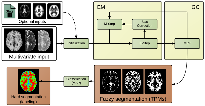
Figure 1: Segmentation flowchart. EM-GC segmentation takes as inputs the blocks depicted in white background and produces the blocks in brown background as outputs. Typically, the initialization can be performed supplying a file with the parameters of the model, or prior TPMs from an atlas (optional inputs are represented with a dashed line connector).

Initialization

Once the model has been fully defined (number of expected pure tissues, number of normal distributions per tissue, number of special PV classes, and bias correction), MBIS allows for several standard initialization approaches. One common and fully-automated strategy is the use of the k-means algorithm, which is the default option in MBIS when no other initialization is required. A second extended initialization strategy is manually setting $\{\theta_{k}\}$, assuming a uniform distribution for $\pi_{k,i}$. Finally, it is also common to use atlas priors when the spatial mapping between the actual case and the atlas is known. Atlas priors can be supplied to MBIS as a set of TPMs, one per normal distribution. It is important to note that these priors are no longer applied after initialization.

Bias correction

When bias correction is required, a new definition of likelihood derived from (1) is applied. We estimate the bias field $B$ approximating the error measurement map $E$ obtained after (3) with uniform B-splines. This solution is dual to N4ITK, the non-parametric algorithm presented elsewhere [tustison_n4itk:_2010]. tustison_n4itk:_2010 analyzed the best B-spline parametrization for bias correction, and concluded that it is preferable to other models based on linear combinations of polynomial or smooth basis functions. Before the next iteration of the E-step (see LABEL:alg:e_m), data are corrected with the field vector ${\mathbf{b}}_{i}$ at $i$ before the distribution parameters are calculated.

partial volume model

On the basis of previous findings [cuadra_comparison_2005], MBIS tackles the PV effect by modeling pure tissues with in-class mixtures of normal distributions, and by adding specific PV classes [noe_partial_2001]. Appropriate transition penalties can be set consistently for these classes, as in [cuadra_comparison_2005]. Instead of estimating the tissue contributions to the PV classes within the model, we provide a simplified procedure to achieve this aim a posteriori. The methodology computes the Mahalanobis distance (7) of the PV samples to the tentative pure tissues. Interpreting the posterior probability as a volume fraction of the tissue within the voxel, this volume is divided between the pure tissues inversely proportional to the distance $D_{k}$ (7) to the tissues. This PV solving is applied to the experimental results presented in section 4.

$$D_{k}({\mathbf{y}}_{i})=\sqrt{({\mathbf{y}}_{i}-\boldsymbol{\mu}_{k})^{T}\boldsymbol{\Sigma}_{k}^{-1}({\mathbf{y}}_{i}-\boldsymbol{\mu}_{k})}.$$ (7)

graph-cuts optimization

MBIS implements GC optimization as in [boykov_fast_2001], wrapping the maxflow library (http://vision.csd.uwo.ca/code/) in ITK (the Insight Registration & Segmentation Toolkit, http://www.itk.org) to solve the graphs. The weighting parameter $\lambda_{\mathcal{N}}$ (4) must be adequately determined for sensible regularization. In section 4.1, we describe the experiment conducted to set $\lambda_{\mathcal{N}}$ empirically. The special PV classes are taken into account specifying an appropriate transition model. The transition model is a matrix where the interactions between individual normal distributions are defined. These energy interactions are defined by the $V_{ij}(x_{i},x_{j})$ presented in section 2.2. Generally, in an MRF model including several normals distributions per tissue (to account for PV effects), transitions within pure tissue have lower penalties (inner transitions) than transitions between pure tissues (outer transitions). MBIS supports complex neighboring systems (beyond the simplest Pott’s model (5)), distance weighted energy interactions, and non-metric tissue transition models.

3 Software description

3.1 Existing software

Many fully automated brain tissue segmentation tools, based on Bayesian classifiers, are readily available and widely used. In Table 1, we present a comparison among representative existing tools, along with a brief summary of the unique features of each. All the tools make use of the MMG model with MRF regularization. The tools listed in the table are FAST [zhang_segmentation_2001], SPM (Statistical Parametric Mapping, The Wellcome Dept. of Imaging Neuroscience, London, UK [ashburner_unified_2005]), EMS (Expectation-Maximization Segmentation [van_leemput_unifying_2003]), ATROPOS [avants_open_2011], NiftySeg [cardoso_niftyseg:_2012], Freesurfer [fischl_freesurfer_2012], and the software proposed in the present study (MBIS). The presented tools generally share a base design that follows the flowchart in Figure 1. It is important to note that Freesurfer and SPM are not just segmentation utilities, but fully automated pipelines for brain MRI processing and analysis that include brain tissue segmentation. SPM provides an isolated interface (called segment) for the problem at hand, the methodology of which is described elsewhere [ashburner_unified_2005]. Conversely, Freesurfer provides precise hard segmentations of the brain in a large number of individual neuroanatomical regions [fischl_whole_2002], which can be appropriately fused to the three-tissue problem. The features presented in Table 1 regarding Freesurfer and SPM refer only to their whole-brain segmentation processes.

Table 1: Brain tissue segmentation tools.

	FAST	SPM	EMS	ATROPOS	NiftySeg	Freesurfer	MBIS
Multivariate	Partial	Partial${}^{1}$	Full	Full	Full	No	Full
Optimization	ICM	ICM	MC	ICM	Unknown	ICM	GC
Bias model	Polynomial	DCT	Polynomial	No${}^{3}$	Unknown	No${}^{3}$	B-spline
Atlas usage	Available	Intensive	Available	Available	Intensive	Intensive	Available
License	GPL	GPL	BSD-like	BSD	BSD	Freeware	GPL
Platform	Unix	Matlab	SPM8	Any${}^{2}$	Any${}^{2}$	Unix	Any${}^{2}$
Reference	[zhang_segmentation_2001]	[ashburner_unified_2005]	[van_leemput_unifying_2003]	[avants_open_2011]	[cardoso_niftyseg:_2012]	[fischl_whole_2002]

${}^{1}$ Work in progress.
${}^{2}$ Any platform supported by the CMake building system.
${}^{3}$ The tool does not integrate a bias model, but it is released along with an external tool for correction.

The first feature to be compared is multivariate implementation. EMS, ATROPOS and NiftySeg fully support the MMG model. SPM is currently integrating support for multivariate data, while FAST provides multichannel segmentation that importantly differs from the univariate segmentation methodology. Freesurfer only supports T1-weighted (T1w) MRI as input for segmentation.

The model estimation is always performed with the EM algorithm, possibly with some improvements. For instance, EMS implements a robust estimator and PV constraints. Therefore, this property has been omitted in Table 1. The main differences are found in the MRF energy minimization problem, ICM being the most used methodology. EMS implements Monte-Carlo (MC)sampling, which is more reliable than ICM but computationally expensive. MBIS is the first tool among the surveyed software packages to include GC optimization, for which a great trade-off between efficiency and correctness has been proven.

Another important feature is the bias field correction, generally solved by approximation of linear combinations of smooth basis functions. FAST and EMS use polynomial least-squares fitting, SPM uses the discrete cosine transform (DCT) with Levenberg-Marquardt (LM) optimization, and MBIS uses B-splines basis. Unfortunately, there was no information available about the bias model implemented in NiftySeg at the time of writing. Two of the surveyed tools do not internally integrate a bias model: Freesurfer provides a pipeline including a previous correction utility, and ATROPOS advises the prior use N4ITK [tustison_n4itk:_2010].

The next point of comparison is the use of atlases to initialize the algorithm and/or to aid the estimation of model parameters. All the tools can initialize segmentation using prior atlas information. Those tools that also use priors throughout the model fitting are denoted with “intensive” atlas use in Table 1.

In terms of software availability, for all the tools the source code is publicly released and the software is distributed under open-source licenses. With respect to their installation, a number of them (FAST, SPM and EMS) are platform-dependent, whereas the others are multi-platform using the CMake building tool (http://www.cmake.org).

3.2 Design considerations

Given the described context of existing software, we aimed to design a multivariate segmentation tool, which is flexible, easy to use, comprehensive, and would also include a GC solver and a B-spline bias field model. As a result we designed MBIS, an open-source and cross-platform software that supports multivariate data by design and that integrates all the methods described in section 2.4. Segmentation provided with MBIS is general purpose. In this study, MBIS is specifically adapted to the 3D brain tissue segmentation problem. In order to facilitate contributions by third-party developers, the code follows the standards of ITK, and some interfaces have been defined to integrate new code, preserving the software modularity.

We also promote reproducible research, a concept that is drawing increasing interest in parallel to the proliferation of computational solutions for image processing problems. Following the definition of vandewalle_reproducible_2009 [vandewalle_reproducible_2009], we release here an open-source bundle with evaluation experiments based on open data to help the community replicate and test our work [yoo_open_2005, ibanez_open_2006].

In order to evaluate MBIS comprehensively, we define three validation targets. Consistently with the design considerations mentioned above, we test the performance of MBIS with three different open data resources containing multivariate and multi-site data. Full details of these databases are provided in LABEL:table:data (LABEL:a:data), describing the MRI sequences involved and their specific parameters. Finally, we address these targets in three different experiments (the results are presented in section 4).

The first experiment evaluates the accuracy of segmentation, with comparison to FAST, using one simulated dataset. The evaluation framework includes tests to calibrate the best parameters for the tool, benchmarks of the bias field estimation, and studies the impact of spatial misalignment between channels. The second experiment evaluates the reproducibility of results, in similar settings to a recent validation study [de_boer_accuracy_2010]. Unfortunately, the database used by de_boer_accuracy_2010 is not publicly available. Hence, the resulting figures are not directly comparable to their work as we used different data. On one hand, we studied the repeatability of the segmentation by analyzing the differences in tissue volumes. On the other hand, the overlap indices described in section 3.3 were evaluated. The third section of the evaluation framework is an exemplary pipeline of tissue volume analysis in large-scale databases. We illustrated the use of MBIS on such applications, segmenting multivariate MRI datasets from 584 healthy subjects, and correlating tissue volumes with age.

3.3 Evaluation framework

The evaluation framework is built using nipype (Neuroimaging in Python, Pipelines, and Interfaces [gorgolewski_nipype:_2011]), in order to facilitate the fulfillment of the requirements of reproducible research. The evaluation includes a nipype Interface to MBIS, three nipype Workflows to implement the experiments described in section 3.2 and a set of scripts in Python to automate the execution of the workflows and presentation of results (figures and tables included in this paper). To assess and compare results appropriately in terms of accuracy and robustness [altman_measurement_1983], we evaluate two families of indicators: volume agreements and overlap indices.

Volume agreement

Volume agreement between the segmentation found and the ground-truth, or between segmentations of corresponding time points, is a commonly used benchmark. Volumes of the identified tissues are directly related to the total size of the brain. Therefore, we provide here the “intra-cranial volume (ICV) fraction” of each tissue as the ratio of the measured volume over the total volume of the whole-brain.

Overlap indices

Overlap is a widely used indicator to assess segmentation results with respect to a ground-truth [crum_generalized_2006]. We use a fuzzy similarity index (fSI) derived from the fuzzy Jaccard’s index (JI) [crum_generalized_2006], as in eq. (8). This fuzzy index definition takes the resulting TPMs as inputs, and naturally extends the binary definition. We refer to the binary index as the similarity index (SI), when computed on hard segmentations. Generally, the definition of JI tends to favor classes with greater volume when computing the average overlap of several classes. Thus, results reporting averages of overlap indices are compensated for tissue volume in this paper. Additional indices are also provided: true-positive fraction (TPF) that acts as a measure of sensitivity (9); extra fraction (EF) that expresses the over-segmentation (10); and overlap conformity measurement (OC), which is reported as an alternative to the SI (11).

$$fSI,SI =\frac{2\,JI}{1+JI}\,,$$ (8)

$$TPF =\frac{TP}{TP+FN}\,,$$ (9)

$$EF =\frac{FP}{TP+FN}\,,$$ (10)

$$OC =1-\frac{FP+FN}{TP}\,,$$ (11)

where $TP$ stands for true positives, $FP$ for false positives, and $FN$ for false negatives. We did not extend these measures to the probabilistic results, so they are only used for the assessment of the hard segmentations.

4 Evaluation experiments and results

4.1 Accuracy assessment and bias field correction

Data

The first experiment demonstrated the accuracy of MBIS, and it was conducted over the only multivariate dataset included in the BrainWeb Simulated Brain Database [cocosco_brainweb:_1997]. The details of this dataset can found in LABEL:table:data. It provides T1w, T2-weighted (T2w) and proton-density-weighted (PDw) realistic MRI, simulated for only one “normal” model presenting a healthy anatomy. We generated the ground-truth taking the TPMs corresponding to soft tissues from the BrainWeb (i.e. CSF, GM, glial matter, and WM). As glial matter and GM are almost indistinguishable (in terms of intensity) for the three MRI (T1w, T2w and PDw), we merged their corresponding TPMs in order to produce a three-class (CSF, GM, and WM) distribution model. The resulting three TPMs were normalized to sum up to 1.0 at every voxel. Using the MAP criterion (2), we generated the ground-truth labeling (presented in the first row of Figure 3). As it is shown in the same figure, the combination of the three TPMs yields a brain mask that was used for brain extraction.

Parameter $\lambda_{\mathcal{N}}$ setting

We characterized the parameter $\lambda_{\mathcal{N}}$ (4), to set an appropriate default value. We used the BrainWeb dataset with a noise factor of 5% and the three available inhomogeneity fields (called 0%, 20% and 40% with increasing strength of intensity non-uniformity field).

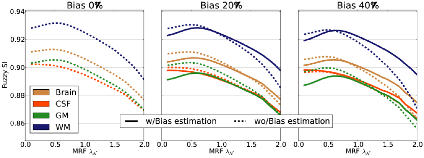
Figure 2: Parameter calibration. Fine tuning of the parameter $\lambda_{\mathcal{N}}$ (4). Dashed lines represent the evaluation without bias estimation and filled lines correspond to the evaluation with bias estimation. The figure shows that the optimum value for $\lambda_{\mathcal{N}}$ ranges [$0.55-0.65$].

From the results shown in Figure 2, two conclusions can be drawn. First, $\lambda_{\mathcal{N}}=[0.55-0.65]$ is consistently the optimum value; and second, the bias estimation does not effectively improve the segmentation results. As the channels have independent inhomogeneity patterns, the model is less prone to this confounding effect, allowing more flexible MMG models without losing sensitivity. This conclusion is confirmed later, on the visual assessment of the estimated bias field maps. Once $\lambda_{\mathcal{N}}$ was set, we explored different PV models to segment the dataset.

Results

The performance test on the synthetic ground-truth was carried out on the three available relaxation-time-weighted sequences (T1w, T2w, and PDw), with 5% noise and 20% bias field. We configured MBIS for fully automatic initialization (k-means) and $\lambda_{\mathcal{N}}=0.6$. Additionally, FAST was also used to perform the segmentation using its multichannel mode and default settings. After evaluating numerous configurations, we achieved acceptable results from FAST with a four-class model as suggested elsewhere [he_generalized_2008]. We merged the TPM of the fourth class into the one corresponding to CSF. This ad hoc decision was taken after ensuring that the accuracy figures were the best we could reach using FAST. The quantitative results shown in Table 2 indicate a better overall performance (row labeled as “Brain”) of MBIS for all the evaluated indices.

Table 2: Quantitative results of the accuracy assessment. Overlap measured using the different indices proposed in section 3.3. Boldface font highlights the best score for both tools at each overlap index. Row labeled as “Brain” represents the volume-corrected average of the three detected clusters (CSF, GM, WM). Columns contain the different indices evaluated (see section 3.3): fuzzy similarity index (fSI), similarity index (SI), true-positive fraction (TPF), extra fraction (EF), and overlap conformity measurement (OC).

		fSI	SI	TPF	EF	OC
	FAST	0.846	0.874	0.907	0.163	0.710
Brain	MBIS	0.912	0.940	0.955	0.079	0.871
	FAST	0.863	0.889	0.993	0.241	0.750
CSF	MBIS	0.900	0.923	0.997	0.163	0.834
	FAST	0.807	0.845	0.741	0.014	0.632
GM	MBIS	0.904	0.939	0.923	0.043	0.871
	FAST	0.868	0.888	0.987	0.236	0.749
WM	MBIS	0.931	0.956	0.945	0.032	0.908

Qualitative evaluation using visual assessment and error maps is also reported. Figure 3 presents representative views of the error maps obtained with the tools under comparison, highlighting regions with remarkable differences.

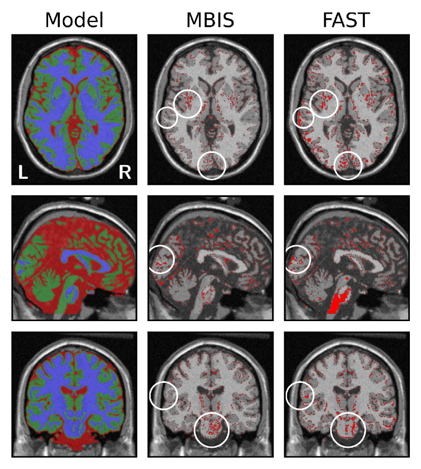
Figure 3: Visual assessment of the hard-segmentation results. The ground-truth is presented on the left column. Error maps are presented for MBIS and FAST (red color represents misclassified pixels). Rather than the obvious differences, we highlighted some more subtle examples.

Regarding the fuzzy outcome, Figure 4 presents the TPMs obtained with MBIS and FAST, compared with the original ones. An error map for each tool under testing is also presented, computed as the voxel-wise mean squared difference between the three original maps and the three maps obtained after segmentation.

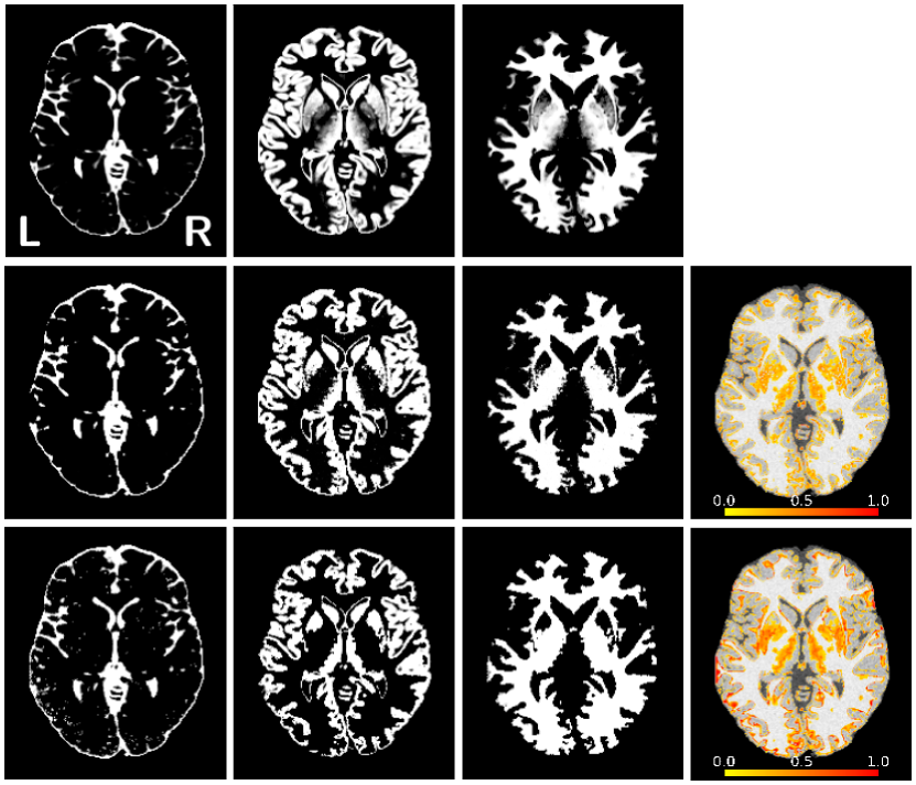
Figure 4: Visual assessment of the fuzzy-segmentation results. First row shows the TPMs of the ground-truth (from left to right: CSF, GM, WM). Second and third rows present the corresponding TPMs obtained with MBIS and FAST, respectively. The extra column represents the mean squared error of the TPMs, normalized by the maximum squared error of both maps.

Bias field estimation

We conclude the accuracy assessment by studying the performance on estimating the bias field. Figure 5 presents a comparison of the results. The first row shows the bias field contained by the simulated data from BrainWeb, for the T1w MRI. The corresponding realizations of bias field for the T2w and PDw images are also available. The second and third rows present the corresponding estimations obtained with MBIS and FAST. Visual assessment is straightforward, as FAST did not perform a valid estimation of the bias field. Similar results were obtained for the bias field that affected the T2w and PDw images. Even though FAST obtained inadequate estimations, segmentation did not lose sensitivity dramatically (see Table 2), confirming that multivariate data are very robust against the different realizations of bias field on each channel, as they are independent.

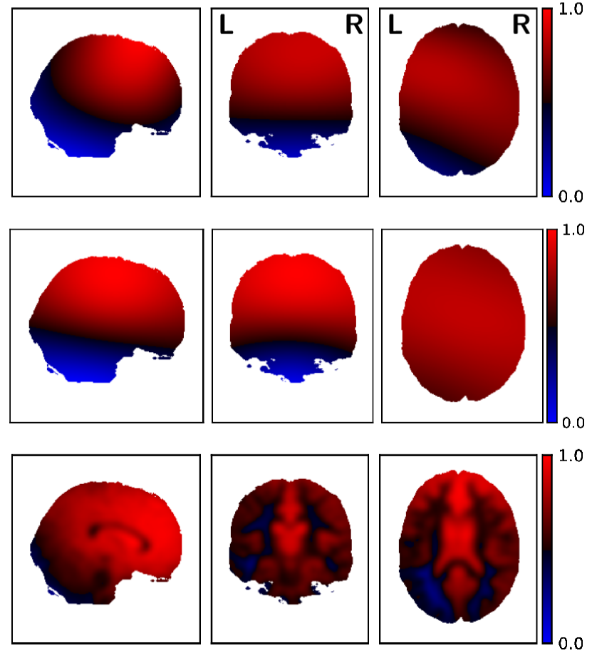
Figure 5: Comparison of bias estimation. Normalized magnitudes of the reference (first row) and estimated field maps are presented (second row is MBIS, third is FAST), for the T1w channel.

Intra-scan registration

The misregistration between the different contrasts stacked as a multivariate image is a prominent drawback that hinders multivariate segmentation. We present in Figure 6 the characterization of the impact of small misalignments between image channels. More precisely, we translated T2w and PDw images from their ground-truth location and conducted multivariate segmentation with MBIS. Segmentation results were assessed using the fSI index, and they were proven to be quite sensitive to the registration error introduced artificially. Given that we restricted the analysis only to 3D translations along the Y-axis, a very important impact should be expected from other misalignments (as rotations, linear transforms of a higher degree, or nonlinear deformations).

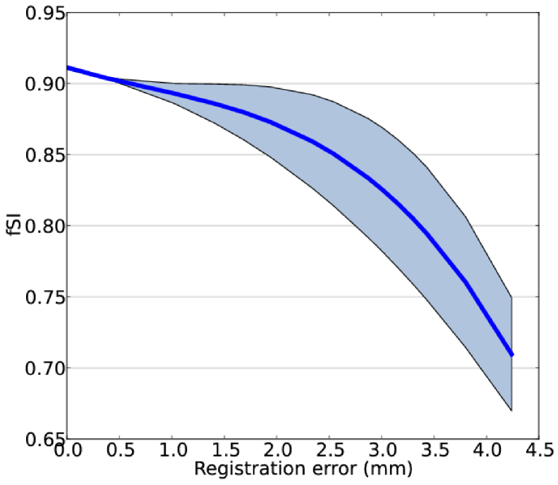
Figure 6: Intra-subject registration error. Influence of different combinations of translations between the channels. The figure represents the fuzzy similarity index (fSI)(defined in section 3.3) versus the absolute displacement.

4.2 Reproducibility evaluation

Data

The Multi-modal MRI Reproducibility Resource (also called the Kirby21 database) [landman_multi-parametric_2011] consists of scan-rescan imaging sessions on 21 healthy volunteers with no history of neurological disease. The database includes a wide range of MRI sequences, from which we selected T1w, T2w and magnetization transfer imaging (MT) for segmentation. The complete database is publicly available online, and details of the MRI sequences and other information can be found in LABEL:table:data.

Image preprocessing

First, all datasets were corrected for inhomogeneity artifacts using N4ITK [tustison_n4itk:_2010] as it was necessary to obtain acceptable brain extraction using BET (Brain Extraction Tool [smith_fast_2002]). Moreover, the use of corrected images as input enabled testing the fully automated initialization included in MBIS, avoiding the use of atlas information. T1w images were then enhanced, replacing intensity values above the 85${}^{th}$ percentile with the local median value. This filtering removed the typical tail present in the intensity distribution of brain-extracted T1w images, corresponding to spurious regions remaining after skull-stripping. The second step, after this initial preparation, consisted of correctly aligning the different modalities with respect to the reference T1w image. We used ANTS (Advanced Normalization Tools [avants_ants:_2013]) to register rigidly the T2w and MT images to the space of the T1w. We visually validated the intra-scan registration of each dataset, as it was proven to be an important source of error hindering repeatability in a previous experiment (section 4.1).

Segmentation

We then used MBIS and FAST to segment the available datasets (a total of 42 datasets from 21 subjects scanned twice), using as input several variations of the three available MRI sequences (i.e. T1w, T2w, and MT). We do not present a comparison of the repeatability with FAST as most of the resulting segmentations from it were not visually acceptable. Even when the results were visually acceptable, they were not repeatable because of the well-known identifiability problem [bishop_pattern_2009]. This problem occurs when a class is correctly detected, but assigned to a different class-identifier, which makes the automatic computation of the evaluation indices impossible. We performed segmentation using MBIS with four different combinations of sequences: T1w alone, T1w-T2w, T1w-MT, and T1w-T2w-MT. The first evaluation considering only the T1w channel is the standard methodology and reference. All segmentation trials used a five-class model, where four represented pure tissues (two for CSF and one each for GM and WM). The remaining class fitted the partial volume existing between CSF and GM. We post-processed the MBIS results to obtain the probability maps corresponding to three-class clustering, as described in section 2.4.

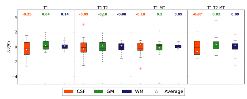
(a) Volume agreement.

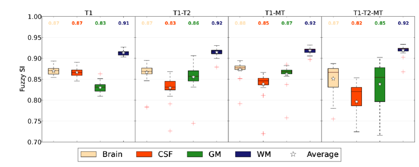
(b) Fuzzy Similarity Index.

Figure 7: Repeatability experiment. Above each subplot, the MRI sequences that were stacked to conduct each segmentation are indicated in the title. For instance, “T1” stands for T1w alone, “T1-T2” stands for T1w and T2w, and so forth. Inside the plots, the median value of each box is on top in the color of the corresponding tissue.

Results

The first experiment consisted of measuring the volume change of each tissue ($\mathrm{\Delta }V{}_{\text{<span title="" class="ltx\_glossaryref"><span class="ltx\_text ltx\_glossary\_name">CSF</span></span>}}$