Groebner basis methods for stationary solutions of a low-dimensional model for a shear flow

Abstract

We use Groebner basis methods to extract all stationary solutions for the 9-mode shear flow model that is described in Moehlis et al, New J. Phys. 6 54 (2004). Using rational approximations to irrational wave numbers and algebraic manipulation techniques we reduce the problem of determining all stationary states to finding roots of a polynomial of order 30. The coefficients differ by 30 powers of 10 so that algorithms for extended precision are needed to extract the roots reliably. We find that there are eight stationary solutions consisting of two distinct states that each appear in four symmetry-related phases. We discuss extensions of these results for other flows.

I Introduction

The transition to turbulence in several shear flows that do not show a linear instability has been connected with the appearance of exact coherent states Faisst and Eckhardt (2003); Wedin and Kerswell (2004); Eckhardt et al. (2007); Eckhardt (2008). These states together with their heteroclinic connections form the scaffold on which the turbulent dynamics takes place Schmiegel (1999); Eckhardt et al. (2008); Gibson et al. (2008a, b); Halcrow et al. (2009) and they dominate the statistical properties of the flow Schneider et al. (2007); Eckhardt et al. (2008); Kerswell and Tutty (2007). In the case of plane Couette flow, a fluid confined between two parallel plates that move in opposite directions, the coherent states are of a particularly simple form because of an up-down symmetry in the flow: they are stationary states Nagata (1990); Clever and Busse (1997); Wang et al. (2007); Schneider et al. (2008). Because of the significance of these states it would be interesting to know how many fixed points there are. In reliable numerical simulations with their thousands of degrees of freedom this amounts to finding zeros of the equations of motion in very high dimensional spaces. The present approaches use suitably adapted Newton methods Viswanath (2007); Dijkstra et al. (2014) to find fixed points in the neighborhood of the initial conditions and therefore cover the state space only probabilistically: as the number of initial conditions tested increases, the room for missed fixed points decreases, which makes their existence less likely but not impossible. Despite these sometimes very costly searches that require millions of initial conditions one is not assured that no pocket with possibly new states is missed. Hence a different approach to finding all states would be welcome. We here discuss how Groebner basis methods Becker and Weispfennig (1993) can be applied to the problem at hand.

The original problem involves a partial differential equation, the Navier-Stokes equation, on a suitably defined domain with appropriate boundary conditions. For this infinite-dimensional system only the simplest solutions can be obtained exactly (like the linear profile for plane Couette flow) and all the ones relevant to the turbulence transition in shear flows are obtained numerically. However, due to the fact that the equation is dissipative and that the fractal dimension of the turbulent state is finite (though increasing with Reynolds number, see Ruelle (1982); Temam (1995)), projections onto finite dimensional subspaces give approximations that become more accurate as the dimensions increase. Within such subspaces, the equations are sufficiently simple and of a form that Groebner basis methods can be used.

Specifically, an expansion of the Navier-Stokes equation in appropriate divergence free basis functions generically leads to coupled equations of the form

$$\dot{a}_{i}=\sum_{j}d_{ij}a_{j}+\sum_{jk}\alpha_{i,jk}a_{j}a_{k}+f_{i}$$ (1)

where the $a_{i}$ are the coefficients for the expansion of the velocity field. The precise form of this representation (in Chandrasekhar modes or spectral-tau schemes or others Gottlieb and Orszag (1977)) only affects the coupling coefficients in the equations and does not matter here. The coefficients $\alpha$ cover the nonlinearity, the $d$’s are typically connected with damping and the $f$’s are external forcings. Formally, the number of equations is infinite because of the partial differential nature of the original equation, and good approximations converge to the exact result as the number of basis functions increases. The conflicting requirement of a large number of modes for numerical accuracy and a small number of modes so that the Groebner basis methods can be applied will be discussed in the concluding section.

The key feature of eq (1) that enables the application of Groebner basis methods is the quadratic coupling between amplitudes. As a consequence, in the generic case, that is, when the system (1) does not have trajectories filled with singular points or, equivalently, the system of polynomials on the right hand side of (1) has only a finite number of zeros, there cannot be more than $2^{N}$ fixed points, where $N$ is the number of equations. The actual number may be obtained by transforming the equations and extracting a Groebner basis. Ultimately, this transforms the problem into one involving the roots of a polynomial in one of the variables, together with equations that determine the remaining variables. The reduction in the number of roots from the maximum of $2^{N}$ comes about because some of the roots may be complex and hence meaningless, and because the final polynomial may be of lower order. Specifically, for the case studied here, we can show that there are only two sets of symmetry related roots.
In the next section we focus the discussion on the 9-mode shear flow model derived in Moehlis et al. (2004, 2005). Section 3 describes the Groebner basis search, and section 4 contains the results for a specific aspect ratio. We conclude with a summary of the results on the present model and an outlook of the implications for other flows in section 5.

II The shear flow model

The 9-mode model used here is obtained for a variation to the original plane Couette flow problem that allows for a representation of the velocity fields in Fourier modes. To this end, the no-slip boundary conditions at the top and bottom plate are replaced by free-slip boundary conditions, and the driving is obtained from a sinusoidal body force. Furthermore, the number of modes is severely truncated so that only nine modes survive. These modes have a physical interpretation, as explained in Moehlis et al. (2004): two modes (amplitudes $a_{1}$ and $a_{9}$) describe the laminar profile and its deformation due to other modes, one mode ($a_{3}$) describes downstream vortices which are important for the extraction of energy from the laminar profile, and another mode ($a_{2}$) then captures the streaks that are induced by the vortices. One pair of modes ($a_{4}$ and $a_{5}$) capture transverse motions that are needed in order to deform the flow in the downstream direction, and another pair ($a_{6}$ and $a_{7}$) describes normal vortices. Finally, there is a 3-d mode ($a_{8}$) that provides important couplings between the modes. For the functional form of the 3-d velocity fields we refer to Moehlis et al. (2004).
The system has three parameters. The control parameter that we will use later on is the Reynolds number $Re$. Two geometrical parameters $\alpha$ and $\gamma$ describe the length $\pi d/\alpha$ and the width $\pi d/\gamma$ of the domains (the height is fixed by $d=2$ with our choice of units). We study the system for the parameter values of the larger of the two domains discussed in Moehlis et al. (2004, 2005), the so-called NBC domain with $\gamma=1$ and $\alpha=1/2$.

Then, the equations for the nine coefficients $a_{1}$, $\dots$, $a_{9}$ are given by:

$$\frac{da_{1}}{dt} = \frac{\beta^{2}}{Re}-\frac{\beta^{2}}{Re}a_{1}-\sqrt{\frac{3}{2}}\left(\frac{\beta}{\kappa_{\alpha\beta\gamma}}a_{6}a_{8}-\frac{\beta}{\kappa_{\beta\gamma}}a_{2}a_{3}\right),$$ (2)

$$\frac{da_{2}}{dt} = -\left(\frac{4\beta^{2}}{3}+1\right)\frac{a_{2}}{Re}+\frac{5\sqrt{2}}{3\sqrt{3}}\frac{1}{\kappa_{\alpha\gamma}}a_{4}a_{6}-\frac{1}{\sqrt{6}\kappa_{\alpha\gamma}}a_{5}a_{7}-\frac{\beta}{2\sqrt{6}\kappa_{\alpha\gamma}\kappa_{\alpha\beta\gamma}}a_{5}a_{8}$$

$$-\sqrt{\frac{3}{2}}\frac{\beta}{\kappa_{\beta\gamma}}(a_{1}a_{3}+a_{3}a_{9}),$$

$$\frac{da_{3}}{dt} = -\frac{\beta^{2}+1}{Re}a_{3}+\frac{1}{\sqrt{6}}\frac{\beta}{\kappa_{\alpha\gamma}\kappa_{\beta\gamma}}(a_{4}a_{7}+a_{5}a_{6})+\frac{7\beta^{2}-15}{4\sqrt{6}\kappa_{\alpha\gamma}\kappa_{\beta\gamma}\kappa_{\alpha\beta\gamma}}a_{4}a_{8},$$ (4)

$$\frac{da_{4}}{dt} = -\frac{3+16\beta^{2}}{12Re}a_{4}-\frac{1}{2\sqrt{6}}(a_{1}a_{5}+a_{5}a_{9})-\frac{5}{6\sqrt{6}}\frac{1}{\kappa_{\alpha\gamma}}a_{2}a_{6}-\sqrt{\frac{3}{2}}\frac{\beta}{2\kappa_{\alpha\gamma}\kappa_{\beta\gamma}}a_{3}a_{7}$$

$$-\sqrt{\frac{3}{2}}\frac{\beta^{2}}{4\kappa_{\alpha\gamma}\kappa_{\beta\gamma}\kappa_{\alpha\beta\gamma}}a_{3}a_{8},$$

$$\frac{da_{5}}{dt} = -\frac{1+4\beta^{2}}{4Re}a_{5}+\frac{1}{2\sqrt{6}}(a_{1}a_{4}+a_{4}a_{9})+\frac{1}{4\sqrt{6}\kappa_{\alpha\gamma}}a_{2}a_{7}-\frac{\beta}{2\sqrt{6}\kappa_{\alpha\gamma}\kappa_{\alpha\beta\gamma}}a_{2}a_{8}$$

$$+\frac{1}{\sqrt{6}}\frac{\beta}{\kappa_{\alpha\gamma}\kappa_{\beta\gamma}}a_{3}a_{6}$$

$$\frac{da_{6}}{dt} = -\frac{15+16\beta^{2}}{12Re}a_{6}+\frac{1}{2\sqrt{6}}(a_{1}a_{7}+a_{7}a_{9})+\sqrt{\frac{3}{2}}\frac{\beta}{\kappa_{\alpha\beta\gamma}}a_{1}a_{8}-\frac{5}{2\sqrt{6}}\frac{1}{\kappa_{\alpha\gamma}}a_{2}a_{4}$$

$$-\sqrt{\frac{2}{3}}\frac{\beta}{\kappa_{\alpha\gamma}\kappa_{\beta\gamma}}a_{3}a_{5}+\sqrt{\frac{3}{2}}\frac{\beta}{\kappa_{\alpha\beta\gamma}}a_{8}a_{9},$$

$$\frac{da_{7}}{dt} = -\frac{5+4\beta^{2}}{4Re}a_{7}-\frac{1}{2\sqrt{6}}(a_{1}a_{6}+a_{6}a_{9})+\frac{3}{4\sqrt{6}}\frac{1}{\kappa_{\alpha\gamma}}a_{2}a_{5}+\frac{1}{2\sqrt{6}}\frac{\beta}{\kappa_{\alpha\gamma}\kappa_{\beta\gamma}}a_{3}a_{4},$$ (8)

$$\frac{da_{8}}{dt} = -\frac{5+4\beta^{2}}{4Re}a_{8}+\frac{1}{\sqrt{6}}\frac{\beta}{\kappa_{\alpha\gamma}\kappa_{\alpha\beta\gamma}}a_{2}a_{5}+\frac{15-4\beta^{2}}{4\sqrt{6}\kappa_{\alpha\gamma}\kappa_{\beta\gamma}\kappa_{\alpha\beta\gamma}}a_{3}a_{4},$$ (9)

$$\frac{da_{9}}{dt} = -\frac{9\beta^{2}}{Re}a_{9}+\sqrt{\frac{3}{2}}\frac{\beta}{\kappa_{\beta\gamma}}a_{2}a_{3}-\sqrt{\frac{3}{2}}\frac{\beta}{\kappa_{\alpha\beta\gamma}}a_{6}a_{8},$$ (10)

where

$$\beta = \frac{\pi}{2},$$ (11)

$$\kappa_{\alpha\gamma} = \sqrt{\alpha^{2}+\gamma^{2}}=\frac{\sqrt{5}}{2},$$ (12)

$$\kappa_{\beta\gamma} = \sqrt{\beta^{2}+\gamma^{2}}=\frac{\sqrt{\pi^{2}+4}}{2},$$ (13)

$$\kappa_{\alpha\beta\gamma} = \sqrt{\alpha^{2}+\beta^{2}+\gamma^{2}}=\frac{\sqrt{\pi^{2}+5}}{2}.$$ (14)

The system (2)-(10) possesses two discrete symmetries that are connected with the invariance of the flow under shifts along half the width and half the length, respectively, in the full domain, Moehlis et al. (2004, 2005):

$$T_{L_{x}/2}\vec{a}=(a_{1},a_{2},a_{3},-a_{4},-a_{5},-a_{6},-a_{7},-a_{8},a_{9}),$$ (15)

$$T_{L_{z}/2}\vec{a}=(a_{1},-a_{2},-a_{3},a_{4},a_{5},-a_{6},-a_{7},-a_{8},a_{9}),$$ (16)

They imply that for each solution $\vec{a}$ there exist another three symmetry-related solutions $T_{L_{x}/2}\vec{a}$, $T_{L_{z}/2}\vec{a}$ and $T_{L_{x}/2}T_{L_{z}/2}\vec{a}$.

The system of these nine modes and their couplings captures many features of shear flows and their dynamical behaviour Moehlis et al. (2004, 2005): the laminar profile is linearly stable for all Reynolds numbers, the non-trivial state that appears first is not a periodic or in other ways simple state but chaotic, and the chaotic dynamics are not persistent but transient. Moreover, the transition scenario between simpler and more complicated states is similar to what has been seen in pipe flow and other shear flows. Of course, it cannot capture the flow behaviour quantitatively because of the small number of modes and hence poor resolution, and it differs from the full system in the boundary conditions.

III Groebner basis

For fixed points $\dot{a}_{i}=0$, and the above equations reduce to a polynomial system of the form

$$f_{1}(a_{1},\dots,a_{n}) = 0,$$

$$\vdots\qquad$$ (17)

$$f_{m}(a_{1},\dots,a_{n}) = 0,$$

where $f_{k}$ are real polynomials and where the roots are the amplitudes of the stationary solutions. Even though such systems of multivariate polynomials are pervasive in all areas of applied science and engineering, no algorithmic methods to solve systems like (III) were known until the mid-sixties of the last century, when Bruno Buchberger Buchberger (1965, 2006); Becker and Weispfennig (1993) invented the theory of Groebner bases. They have since become the cornerstone of modern computational algebra.

We here summarize the notion of Groebner basis briefly and refer to Buchberger (1965, 2006); Becker and Weispfennig (1993); Arnold (2003) for more details. Let $k[a_{1},\dots,a_{n}]$ denote the ring of polynomials of variables $a_{1},\dots,a_{n}$ with coefficients in a field $k$ and $I=\langle f_{1},f_{2},\dots,f_{s}\rangle$ denote the ideal generated by polynomials $f_{1}(a_{1},\dots,a_{n})$, $\ldots$, $f_{s}(a_{1},\dots,a_{n})$, that is, the set of all sums $\{h_{1}f_{1}+h_{2}f_{2}+\dots+h_{s}f_{s}\},$ where $f_{k},h_{k}$ are polynomials.

A Groebner basis of $I$ requires an ordering of the monomials of $k[a_{1},\dots,a_{n}]$, and different orderings give different results. The two most commonly used term orders are the lexicographic order and the degree reverse lexicographic order, defined as follows. Let $\mu=(\mu_{1},\dots,\ \mu_{n})$ and $\nu=(\nu_{1},\dots,\nu_{n})$ be elements of $\mathbb{N}_{0}^{n}$ ($\mathbb{N}_{0}=\mathbb{N}\cup 0$). We say that $\mu\succ_{\rm lex}\nu$ with respect to the lexicographic order if and only if, reading left to right, the first nonzero entry in the $n$-tuple $\mu-\nu\in\mathbb{Z}^{n}$ is positive. Similarly, we say that $\mu\succ_{\rm degrev}\nu$ with respect to the degree reverse lexicographic order if and only if $|\mu|=\sum_{j=1}^{n}\mu_{j}>|\nu|=\sum_{j=1}^{n}\nu_{j}$ or $|\mu|=|\nu|\$ and, reading right to left, the first nonzero entry in the $n$-tuple $\mu-\nu\in\mathbb{Z}^{n}$ is negative.

Furthermore, we introduce the abbreviated notation ${\bf a}^{\sigma}$ for the monomial $a_{1}^{\sigma_{1}}a_{2}^{\sigma_{2}}\cdots a_{n}^{\sigma_{n}}$ with $\sigma\in\mathbb{N}_{0}$. Fixing a term order on $k[a_{1},\dots,a_{n}]$, any $f\in k[a_{1},\dots,a_{n}]$ may then be written in the standard form with respect to the order,

$$f=\alpha_{1}{\bf a}^{\mu_{1}}+\alpha_{2}{\bf a}^{\mu_{2}}+\dots+\alpha_{s}{\bf a}^{\mu_{s}},$$ (18)

where $\mu_{i}\neq\mu_{j}$ for $i\neq j$ and $1\leq i,j\leq s$, and where, with respect to the specified term order, $\mu_{1}\succ\mu_{2}\succ\cdots\succ\mu_{s}$. The leading term $LT(f)$ of $f$ is the term $LT(f)=\alpha_{1}{\bf a}^{\mu_{1}}$.

Let $f$ and $g$ be from $k[a_{1},\dots,a_{n}]$ with $LT(f)=\alpha{\bf a}^{\mu}$ and $LT(g)=\beta{\bf a}^{\nu}$. The least common multiple of ${\bf a}^{\mu}$ and ${\bf a}^{\nu}$, denoted $LCM({\bf a}^{\mu},{\bf a}^{\nu})$, is the monomial ${\bf a}^{\sigma}=a_{1}^{\sigma_{1}}\cdots a_{n}^{\sigma_{n}}$ such that $\sigma_{j}=\max(\mu_{j},\nu_{j})$, $1\leq j\leq n$, and the $S$-polynomial of $f$ and $g$ is the polynomial

$$S(f,g)=\frac{{\bf a}^{\sigma}}{LT(f)}f-\frac{{\bf a}^{\sigma}}{LT(g)}g.$$

The following algorithm due to Buchberger Buchberger (1965) produces a Groebner basis $G=\{g_{1},\dots,g_{s}\}$ for the ideal $I=\langle f_{1},\dots,f_{s}\rangle\in k[a_{1},\dots,a_{n}]$:

• Step 1: $G:=\{f_{1},\dots,f_{s}\}$.
  

• Step 2: For each pair $g_{i},g_{j}\in G$, $i\neq j$, compute the $S$-polynomial $S(g_{i},g_{j})$ and compute the remainder $r_{ij}$ of the division $S(g_{i},g_{j})$ by $G$.
  

• Step 3: If all $r_{ij}$ are equal to zero, output $G$,
  else
  add all nonzero $r_{ij}$ to $G$ and return to Step 2.

It is clear that the set of solutions of the system

$$g_{1}=\dots=g_{s}=0$$

is the same as the set of solutions of the original system (III).

The convergence criterion in the last step requires that the coefficients vanish exactly. This can only be met if the coefficients of the polynomials are integers or rational numbers (which become integers once the equation is multiplied with the least common multiple of all denominators).

A Groebner basis $G=\{g_{1},\dots,g_{m}\}$ is called reduced if for all $i$, $1\leq i\leq m$, the coefficient of the leading term is 1 and no term of $g_{i}$ is divisible by any $LT(g_{j})$ for $j\neq i$. It is well known (see e.g. Cox et al. (1997); Romanovski and Shafer (2009)) that system (III) has a solution over the field of complex numbers if and only if the reduced Groebner basis $G$ for $\langle f_{1},\dots,f_{s}\rangle$ with respect to any term order on $\mathbb{C}[a_{1},\dots,a_{n}]$ is different from $\{1\}$. The Groebner basis theory allows to find all solutions of system (III) in the case the system has only a finite number of solutions. In such case a Groebner basis with respect to the lexicographic order is always in a “triangular” form.

If system (III) has only a finite number of solutions, then any reduced Groebner basis with respect to a lexicographic order must contain a polynomial in one variable, say, $g_{1}(a_{1})$. Then, there is a group of polynomials in the Groebner basis depending on this variable and one more variable, say, $g_{2}(a_{1},a_{2}),\dots,g_{t}(a_{1},a_{2})$ etc. Thus, we first solve (perhaps numerically) the equation $g_{1}(a_{1})=0$. Then, for each solution $a_{1}^{*}$ of $g_{1}(a_{1})=0$ we find the solutions of $g_{2}(a_{1}^{*},a_{2})=\dots=g_{t}(a_{1}^{*},a_{2})=0,$ which is a system of polynomials in a single variable $a_{2}$. Continuing the process we obtain in this way all solutions of our system (III). Therefore, in the case of a finite number of solutions, Groebner basis computations provide the complete solution to the problem (see e.g. Cox et al. (1997) for more details). However, this theoretical result is in practice clouded by considerable technical difficulties, since calculations of Groebner bases, especially with respect to lexicographic orders, require tremendous computational resources, as the size of the coefficients of $S$-polynomials grows exponentially during the execution of the algorithms.

Therefore, the computation of Groebner bases requires powerful computers and efficient program packages. Nowadays all major computer algebra systems (Mathematica, Maple, REDUCE, SINGULAR, Macaulay and many others) have routines to compute Groebner bases, which use much more efficient algorithms than the original ones described above. To our experience one of the most efficient software tools for this purpose is the computer algebra system SINGULAR Greuel et al. (2005) because of its rich functionality and high performance in implementation of constructive algorithms. In our study of the system (2)-(10) we were able to complete the computation over the field of the rational numbers.

As mentioned, Groebner bases cannot be calculated over real numbers, so all irrational numbers have to be approximated by rational ones. The Reynolds numbers we study are between 200 and 1000 and are taken to be integers. The geometrical factors and the coupling contain irrational numbers that have to be approximated by ratios. We noticed that poor approximations gave results incompatible with numerical simulations of the full equations, so we finally settled for the representations

$$\alpha=1/2,\quad\beta=157/100\approx\frac{\pi}{2},\quad\gamma=1$$

and

$$\sqrt{3/2}\approx 564597/460992,\quad\sqrt{2/3}\approx 837390/1025589,$$

$$\sqrt{6}\approx 1590187/649191,$$

$$\kappa_{\alpha\gamma}\approx 1934705/1730453,\quad\kappa_{\beta\gamma}\approx 1441913/774629,$$

$$\kappa_{\alpha\beta\gamma}\approx 334287/173438.$$

IV Results for the shear flow model

The Groebner bases of the 9-mode shear flow model were determined for Reynolds numbers 200, 300, 350, 400, 500 and 1000 (each Reynolds number required an independent determination of the basis). In each case we found a basis consisting of 11 polynomials, with one of them, $j_{1}(a_{9})$, depending on $a_{9}$ only, and the others containing $a_{9}$ and one or more of the other coefficients. Therefore, the roots of $j_{1}$ define the possible values of $a_{9}$ and the other equations give the values for the other coefficients, or, if no real solutions can be found, eliminate a particular root of $j_{1}$. The fixed points of the 9-mode shear flow model are mapped equivalently to the roots of polynomials on the right hand side of (1) and the roots are determined by computing the reduced Groebner basis of the polynomials using the lexicographic ordering with $a_{1}\succ a_{2}\succ a_{3}\succ a_{4}\succ a_{5}\succ a_{6}\succ a_{7}\succ a_{8}\succ a_{9}$. The Groebner basis found for the 9-mode shear flow model generally has the following structure:

$$j_{1}(a_{9})\; =\;a_{9}\;p_{1}(a_{9})$$ (19)

$$j_{2}(a_{8},a_{9})\; =\;a_{8}\;p_{2}(a_{9})$$ (20)

$$j_{3}(a_{8},a_{9})\; =\;c_{3}\;(a_{8})^{2}\;+\;p_{3}(a_{9})$$ (21)

$$j_{4}(a_{7},a_{8},a_{9})\; =\;c_{4}\;a_{7}\;+\;a_{8}\;+\;p_{4}(a_{9})$$ (22)

$$j_{5}(a_{6},a_{8},a_{9})\; =\;c_{5}\;a_{6}\;+\;a_{8}\;p_{5}(a_{9})$$ (23)

$$j_{6}(a_{5},a_{9})\; =\;a_{5}\;p_{6}(a_{9})$$ (24)

$$j_{7}(a_{5},a_{9})\; =c_{7}\;(a_{5})^{2}\;+\;p_{7}(a_{9})$$ (25)

$$j_{8}(a_{4},a_{5},a_{9})\; =\;c_{8}\;a_{4}\;+\;a_{5}\;a_{8}\;p_{8}(a_{9})$$ (26)

$$j_{9}(a_{3},a_{5},a_{8},a_{9})\; =\;c_{9}\;a_{3}\;+\;a_{5}\;a_{8}\;p_{9}(a_{9})$$ (27)

$$j_{10}(a_{2},a_{5},a_{8},a_{9})\; =\;c_{10}\;a_{2}\;+\;a_{5}\;a_{8}\;p_{10}(a_{9})$$ (28)

$$j_{11}(a_{1},a_{9})\; =\;a_{1}\;-\;9\;a_{9}\;-\;1$$ (29)

with coefficients $c_{3}$ to $c_{10}$ and the polynomials

$$p_{\nu}(a_{9})=\sum_{\mu=0}^{30}\alpha_{\nu\mu}(a_{9})^{\mu}.$$ (30)

The coefficients $c_{\nu}$ and the polynomial coefficients $\alpha_{\nu\mu}$ depend on the Reynolds number, but the structure of the Groebner basis does not.

These coefficients are integer numbers of enormous size and varying signs. For instance, for $Re=400$ the coefficients $\alpha_{2j}$ have more than 1300 digits and vary over up to 29 orders of magnitude,

$$\left|\frac{\alpha_{2,25}}{\alpha_{2,0}}\right|\approx\frac{1.23\cdot 10^{1315}}{4.98\cdot 10^{1285}}\approx 2.5\cdot 10^{29}.$$ (31)

Together with alternating signs this causes enormous cancellations and considerable numerical difficulties. This applies in particular in the regions of most interest, where the roots of the polynomials are located, e.g. $p_{2}(a_{9})$ with $a_{9}\in[-1,1]$. For example, $a_{9}=10^{-1}$ results in $(a_{9})^{30}=10^{-30}$, which is a variation by $30$ orders of magnitude in the powers of the variable alone. In order to overcome this problem arbitrary precision algorithms of the ”Class library for numbers” (CLN) are used to compute the functional values of the polynomials using the Horner algorithm. The number of reliable digits of CLN floating point numbers can be tuned to any desired accuracy Haible and Kreckel (2008). The implementation of elementary arithmetics of the CLN is remarkably fast, so that root finding for the polynomial $p_{2}(a_{9})$ by Newton’s method is just a matter of seconds even when numbers with thousands of digits have to be handled.

For our case, where the coefficients vary by about 30 orders of magnitude, we found that 55 significant digits are sufficient to determine the real roots of the 9-mode model up to a relative error of approximately $10^{-4}$ using Newtons method. This is of the same order as the error introduced by representing the real coefficients of the 9-mode model by rationals needed for the Groebner basis. To be on the safe side for all parameter values, we worked with 100 digits, so that the roots could be determined with at least 30 reliable digits.

It is not only the range that is large, but the absolute numbers as well. The coefficients in the Groebner basis can be as large as $10^{27000}$. For instance, when we plot the polynominal $p_{2}(a_{9})$ in Figure 1, we use the decadic logarithm $\lg|p_{2}(a_{9})|$ to cover values up to $\mathcal{O}(10^{1300})$. The roots of the polynomial result in logarithmic singularities in this diagram, which are easily identified in the otherwise smooth function.

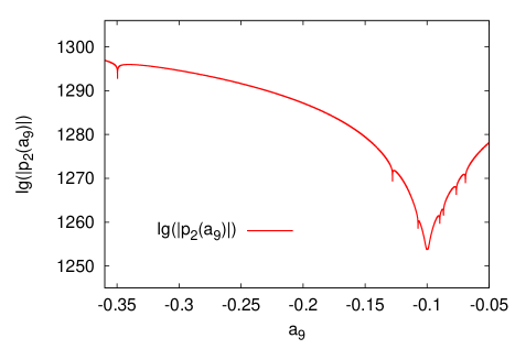
Figure 1: The decadic logarithm of the value of the polynomial $p_{2}(a_{9})$ reveals roots as logarithmic singularities, which are easily identified in the plot. From left to right there are 3 roots followed by an extremum and another four roots.

The polynomial $p_{2}(a_{9})$ and thus also the polynomial $j_{2}(a_{8},a_{9})$ possess exactly 8 roots in variable $a_{9}$ indicated by $a^{\prime}_{9,s}$ with $s\in\{1,2,\ldots,8\}$. The polynomials $p_{1}$ and $p_{6}$ coincide with $p_{2}$. From polynomials $j_{3}(a_{8},{a^{\prime}_{9,s}})$ and $j_{7}(a_{5},{a^{\prime}_{9,s}})$ necessarily follow values for the roots $a^{\prime}_{8,s,t}$ and $a^{\prime}_{5,s,t}$ of these polynomials with $t\in\{1,2\}$, the multiplicity is due to the free choice in sign. The quadratic occurrence of $a_{8}$ and $a_{5}$ in these polynomials suggests that there are up to four times eight real roots

$$a^{\prime}_{8,s,t}=\pm\sqrt{-\frac{p_{3}(a^{\prime}_{9,s})}{c_{3}}}$$ (32)

and

$$a^{\prime}_{5,s,t}=\pm\sqrt{-\frac{p_{7}(a^{\prime}_{9,s})}{c_{7}}}$$ (33)

in these variables. Interestingly, not all roots $a^{\prime}_{9,s}$ result in real values of $a^{\prime}_{8,s,t}$ and $a^{\prime}_{5,s,t}$, which indicates that not all roots of $j_{2}(a_{8},a_{9})$ belong to a set of common roots $\{a_{\mu,r}\}$ of the Groebner basis $j_{\nu}(\{a_{\mu}\})$. Table 1 shows the hierarchy of resulting roots of $j_{2}$, $j_{3}$ and $j_{7}$ followed by their implications on the Groebner basis.

Table 1: The roots $a^{\prime}_{9,s}$ of polynomial $j_{2}(a_{8},a_{9})$ and the resulting values of $a^{\prime}_{8,s,t}$ and $a^{\prime}_{5,s,t}$ indicate that only two roots of $j_{2}(a_{8},a_{9})$ belong to a set of common roots of the Groebner basis.

s	$a^{\prime}_{9,s}$	$a^{\prime}_{8,s,t}$	$a^{\prime}_{5,s,t}$	Root of Groebner basis
1	$-0.350$	$\pm 0.827$	$\not\in\mathbb{R}$	No
2	$-0.128$	$\pm 2.13$	$\not\in\mathbb{R}$	No
3	$-0.107$	$\not\in\mathbb{R}$		No
4	$-0.0897$	$\pm 0.0631$	$\pm 0.0356$	Yes
5	$-0.0868$	$\not\in\mathbb{R}$		No
6	$-0.0764$	$\pm 0.0734$	$\pm 0.0771$	Yes
7	$-0.0691$	$\pm 2.25$	$\not\in\mathbb{R}$	No
8	$0.00924$	$\pm 0.00414$	$\not\in\mathbb{R}$	No

The structure of the Groebner basis clearly reveals that all the remaining polynomials do not impose further restrictions on the two roots $a_{9,4}$ and $a_{9,6}$ such that each of these roots of $j_{2}(a_{8},a_{9})$ gives rise to a real root of the Groebner basis. The remaining $j_{\nu}({a_{\mu}})$ can successively be solved for the remaining undetermined $a_{\mu}$, which are then uniquely determined once the signs of $a_{8}$ and $a_{5}$ have been chosen.

Table 2 lists all eight roots of the Groebner basis of the 9-mode shear flow model at Reynolds number $Re=400$. The different roots of the Groebner basis follow from the signs of the roots $a^{\prime}_{9,4}$ and $a^{\prime}_{9,6}$ of polynomial $j_{2}(a_{8},a_{9})$. From the theory of Groebner bases discussed above these sets of variables are equivalent to fixed points of the 9-mode shear flow model, which will be investigated in the following.

Table 2: A list of all eight roots of the Groebner basis at $Re=400$ following from the roots $a^{\prime}_{9,4}$ (top) and $a^{\prime}_{9,6}$ (bottom) of polynomial $j_{2}(a_{8},a_{9})$. A root of the Groebner basis consists of a column of signs multiplied to the column of values. The four sets of signs follow from Equations (32) and (33). The values of the $\{a_{\mu}\}$ have been computed much more accurately than displayed and have been truncated for this list.

$r$	1	2	3	4
$a^{\prime}_{8,4}$	$>0$	$<0$	$>0$	$<0$
$a^{\prime}_{5,4}$	$>0$	$>0$	$<0$	$<0$
$a_{9,r}$					-0.0897 ​44635 ​37647
$a_{8,r}$	+	-	+	-	0.0631 ​22811 ​60210
$a_{7,r}$	-	+	-	+	0.1794 ​15620 ​62289
$a_{6,r}$	+	-	+	-	0.1063 ​13203 ​79275
$a_{5,r}$	+	+	-	-	0.0356 ​35231 ​54453
$a_{4,r}$	+	+	-	-	0.0168 ​03142 ​01677
$a_{3,r}$	+	-	-	+	0.0345 ​33570 ​69306
$a_{2,r}$	+	-	-	+	0.0481 ​49018 ​20195
$a_{1,r}$	+	+	+	+	0.1922 ​98281 ​61171
r	5	6	7	8
$a^{\prime}_{8,6}$	$>0$	$<0$	$>0$	$<0$
$a^{\prime}_{5,6}$	$>0$	$>0$	$<0$	$<0$
$a_{9,r}$					-0.0764 ​45389 ​20741
$a_{8,r}$	+	-	+	-	0.0734 ​20744 ​07881
$a_{7,r}$	-	+	-	+	0.2989 ​49154 ​13129
$a_{6,r}$	+	-	+	-	0.0711 ​93885 ​61847
$a_{5,r}$	+	+	-	-	0.0771 ​37476 ​48830
$a_{4,r}$	+	+	-	-	0.0157 ​42387 ​67594
$a_{3,r}$	+	-	-	+	0.0355 ​82985 ​62015
$a_{2,r}$	+	-	-	+	0.0265 ​26551 ​11492
$a_{1,r}$	+	+	+	+	0.3119 ​91497 ​13324

Given the numerical difficulties with the polynomials we verified the roots by substituting them into the equations of motion (with ordinary double precision floating point arithmetic). We find that all roots of the Groebner basis listed in Table 2 are indeed fixed points of the 9-mode shear flow model. The different sign combinations mirror the symmetry relations of the amplitude equations.

The physical states corresponding to the fixed points of the 9-mode shear flow model are functions of the Reynolds number. It is relatively straightforward to track the roots, once they have been determined for one Reynolds number, to different Re. A gradual decrease of the Reynolds number shows that the fixed points do not vary much with the Reynolds number until it reaches $Re\approx 308.17$, where the coefficients quickly approach each other and annihilate in an inverse saddle node bifurcation, as shown in Figure 2.

As the Groebner basis has been determined for $Re=400$ it is guaranteed that there exist just the eight fixed points found for exactly this Reynolds number. In principle there could exist more fixed points for other Re, not connected to the ones identified through bifurcations. We therefore computed Groebner bases for $Re=\{200,300,350,500,1000\}$. For the lowest two values $Re=200$ and $Re=300$ the Groebner bases do not posses any roots besides the trivial one, so there are no fixed points and stationary solutions in this flow regime. For all other Reynolds numbers there exist exactly eight roots of the Groebner basis as is the case for $Re=400$ and the corresponding fixed points are identical to those obtained from root tracking. From these checks we conclude that there exist only eight fixed points of the 9-mode shear flow model in this range of Reynolds numbers.

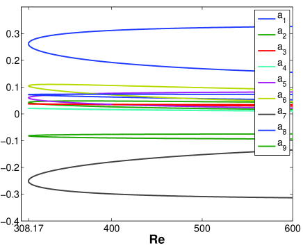
Figure 2: The bifurcation diagram shows the merging of the fixed points $\{a_{\mu,1}\}$ and $\{a_{\mu,5}\}$ of the 9-mode shear flow model at the critical Reynolds number $Re_{crit}=308.17$.

To conclude this section, we display the velocity field of the fixed point that has been obtained by these methods, at the point of bifurcation at $Re=308.17$. One clearly notes the pair of vortices and the modulations in the downstream velocity, the streaks. As one moves above the critical Reynolds number for the bifurcation, the upper and lower branch differ slightly in the velocity pattern from the one at the point of bifurcation, but the vortices and streaks remain prominent features.

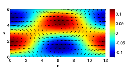
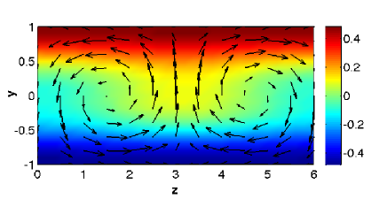
Figure 3: Velocity field of one fixed point at the saddle-node bifurcation at $Re\approx 308.17$. Left image: Flow in the midplane of the domain ($y=0$). The color indicates the velocity in $y$-direction and the arrows indicate the flow in the $(x,z)$-plane. Right image: The color and the arrows indicate the averaged flow in $x$-direction and the flow in the $(y,z)$-plane, respectively.

V Conclusions

The Groebner basis analysis has confirmed that the two sets of four symmetry related fixed points found numerically in Moehlis et al. (2005) are indeed the only ones in this setting. They appear in a saddle node bifurcation near $Re=308.17$ and continue to exist for all larger Reynolds numbers. The absence of further fixed points at higher Reynolds numbers is somewhat unexpected, especially in view of the high degree of the polynominal and the large number of additional states found in direct numerical simulations of the full system Schmiegel (1999); Gibson et al. (2008b). However, all these states have a more complicated spatial structure that cannot be captured by the simple Fourier modes included in the present model. This suggests that more states can only be found if the model is extended to include additional spatial degrees of freedom that can become dynamically active.

As in other cases, the dynamics of the Groebner basis calculation remains mysterious and unpredictable. On top of that, the calculation of roots of polynomials of order 30 with coefficients O(1) near the origin turns out to be unexpectedly troubling, requiring very high precision arithmetic. The dependence on the parameters, in particular the aspect ratio and the Reynolds number seems to be sufficiently well behaved, at least for the aspect ratios studied here. This also suggests that the rational approximation of real quantities that is required for the Groebner analysis can be tolerated.

Given the complexity of the calculation one would like to take advantage of as much prior information as possible, and include, for instance, the discrete symmetries. The four-fold discrete degeneracy of the solutions shows up in the quadratic equations for $a_{8}$ and $a_{5}$ in equations (32) and (33), respectively. However, we are not aware of methods that would allow to include this in a Groebner basis algorithm.

The existence of stationary solutions is a special feature of plane Couette flow, connected with the discrete up-down symmetry of the velocity field Nagata (1990); Clever and Busse (1997); Wang et al. (2007). Once this symmetry is broken the states move downstream in the form of traveling waves. In more general cases, like plane Poiseuille flow or pipe flow, no stationary solutions can exist and travelling waves are the simplest states that can appear Faisst and Eckhardt (2003); Wedin and Kerswell (2004). Since travelling waves become fixed points in a co-moving frame of reference, a similar analysis should be possible at the expense of yet another parameter, the phase speed of the solutions. Now the issue would be to find the number of solutions for a given Reynolds number and all possible phase speeds. This requires either multiple transformations for a set of phase speeds (similar to the scan of Reynolds numbers discussed in section 2) or the analysis of a higher order system with the phase speed as an additional parameter.

Acknowledgements. This work was partly supported by the Deutsche Forschungsgemeinschaft with Forschergruppe 1182. VR acknowledges the support by the Slovenian Research Agency and by the Transnational Access Programme at RISC-Linz of the European Commission Framework 6 Programme for Integrated Infrastructures Initiatives under the project SCIEnce (contract no. 026133).

References

- Faisst and Eckhardt (2003) H. Faisst and B. Eckhardt, Phys. Rev. Lett. 91, 224502 (2003).
- Wedin and Kerswell (2004) H. Wedin and R. R. Kerswell, J. Fluid Mech. 508, 333 (2004).
- Eckhardt et al. (2007) B. Eckhardt, T. M. Schneider, B. Hof, and J. Westerweel, Annu. Rev. Fluid Mech. 39, 447 (2007).
- Eckhardt (2008) B. Eckhardt, Nonlinearity 21, T1 (2008).
- Schmiegel (1999) A. Schmiegel, Transition to turbulence in linearly stable shear flows, Ph.D. thesis, Philipps-Universität Marburg (1999).
- Eckhardt et al. (2008) B. Eckhardt, H. Faisst, A. Schmiegel, and T. M. Schneider, Phil. Trans. R. Soc. A 366, 1297 (2008).
- Gibson et al. (2008a) J. F. Gibson, J. Halcrow, and P. Cvitanović, J. Fluid Mech. 611, 107 (2008a).
- Gibson et al. (2008b) J. F. Gibson, J. Halcrow, and P. Cvitanović, J. Fluid Mech. 638, 23 (2008b).
- Halcrow et al. (2009) J. Halcrow, J. F. Gibson, P. Cvitanović, and D. Viswanath, J. Fluid Mech. 621, 365 (2009).
- Schneider et al. (2007) T. M. Schneider, B. Eckhardt, and J. Vollmer, Phys. Rev. E 75, 066313 (2007).
- Kerswell and Tutty (2007) R. R. Kerswell and O. R. Tutty, J. Fluid Mech. 584, 69 (2007).
- Nagata (1990) M. Nagata, J. Fluid Mech. 217, 519 (1990).
- Clever and Busse (1997) R. M. Clever and F. H. Busse, J. Fluid Mech. 344, 137 (1997).
- Wang et al. (2007) J. Wang, J. F. Gibson, and F. Waleffe, Phys. Rev. Lett. 98, 6 (2007).
- Schneider et al. (2008) T. M. Schneider, J. F. Gibson, M. Lagha, F. De Lillo, and B. Eckhardt, Phys. Rev. E 78, 037301 (2008).
- Viswanath (2007) D. Viswanath, J. Fluid Mech. 580, 339 (2007).
- Dijkstra et al. (2014) H. A. Dijkstra, F. W. Wubs, A. K. Cliffe, E. Doedel, I. F. Dragomirescu, B. Eckhardt, A. Y. Gelfgat, A. L. Hazel, V. Lucarini, A. G. Salinger, E. T. Phipps, J. Sanchez-Umbria, H. Schutrelaars, L. S. Tuckerman, and U. Thiele, Commun. Comput. Phys. 15, 1 (2014).
- Becker and Weispfennig (1993) T. Becker and V. Weispfennig, Gröbner bases: a computational approach to commutative algebra, Graduate Texts in Mathematics, Vol. 141 (Springer, 1993).
- Ruelle (1982) D. Ruelle, Comm. Math. Phys. 87, 287 (1982).
- Temam (1995) R. Temam, Navier-Stokes equations and nonlinear functional analysis (SIAM, 1995).
- Gottlieb and Orszag (1977) D. Gottlieb and S. Orszag, Numerical Analysis of Spectral Methods: Theory and Applications, CBMS-NSF Regional Conference Series in Applied Mathematics (Society for Industrial and Applied Mathematics, 1977).
- Moehlis et al. (2004) J. Moehlis, H. Faisst, and B. Eckhardt, New J. Phys. 6, 56 (2004).
- Moehlis et al. (2005) J. Moehlis, H. Faisst, and B. Eckhardt, SIAM J. Appl. Dyn. Syst. 4, 352 (2005).
- Buchberger (1965) B. Buchberger, Ein Algorithmus zum Auffinden der Basiselemente des Restklassenringes nach einem nulldimensionalen Polynomideal, Ph.D. thesis, University of Innsbruck (1965).
- Buchberger (2006) B. Buchberger, J. Symbolic Comput. 41, 475 (2006).
- Arnold (2003) E. A. Arnold, J. Symbolic Comput. 35, 403 (2003).
- Cox et al. (1997) D. Cox, J. Little, and D. O’Shea, Ideals, Varieties, and Algorithms (Springer, 1997).
- Romanovski and Shafer (2009) V. G. Romanovski and D. S. Shafer, The center and cyclicity problems: a computational algebra approach (Birkhäuser, 2009).
- Greuel et al. (2005) G.-M. Greuel, G. Pfister, and H. Schönemann, Singular 3.0 A computer algebra system for polynomial computations, Tech. Rep. (University of Kaiserslautern, www.singular.uni-kl.de, 2005).
- Haible and Kreckel (2008) B. Haible and R. B. Kreckel, “CLN, a class library for numbers,” www.ginac.de/CLN (2008).