A Multiscale Thermo-Fluid Computational Model
for a Two-Phase Cooling System

Abstract

In this paper, we describe a mathematical model and a numerical simulation method for the condenser component of a novel two-phase thermosyphon cooling system for power electronics applications. The condenser consists of a set of roll-bonded vertically mounted fins among which air flows by either natural or forced convection. In order to deepen the understanding of the mechanisms that determine the performance of the condenser and to facilitate the further optimization of its industrial design, a multiscale approach is developed to reduce as much as possible the complexity of the simulation code while maintaining reasonable predictive accuracy. To this end, heat diffusion in the fins and its convective transport in air are modeled as 2D processes while the flow of the two-phase coolant within the fins is modeled as a 1D network of pipes. For the numerical solution of the resulting equations, a Dual Mixed-Finite Volume scheme with Exponential Fitting stabilization is used for 2D heat diffusion and convection while a Primal Mixed Finite Element discretization method with upwind stabilization is used for the 1D coolant flow. The mathematical model and the numerical method are validated through extensive simulations of realistic device structures which prove to be in excellent agreement with available experimental data.

1 Introduction and Motivation

Ever since the early 1980s the increasing growth of new technologies and applications has been shifting scientific interest on power electronics. In such wide-range industrial context, the necessity to develop devices with a high power dissipation per unit volume has justified the need of advanced cooling systems capable to prevent excessive temperature increase and consequent device failure. Conventional cooling procedures exploit convection heat transfer between a fluid in motion and a bounding surface at different temperatures. Typical examples are water-cooled and air-cooled systems, widely used in power electronics applications. A different approach to cooling is represented by the two-phase thermosyphon device whose functioning principle is schematically illustrated in Fig. 1 and whose structure is shown in Fig. 2(a).

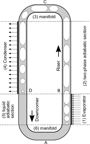
Figure 1: Schematic representation of the working principle of a thermosyphon cooler.

(a) Cooling system assembly

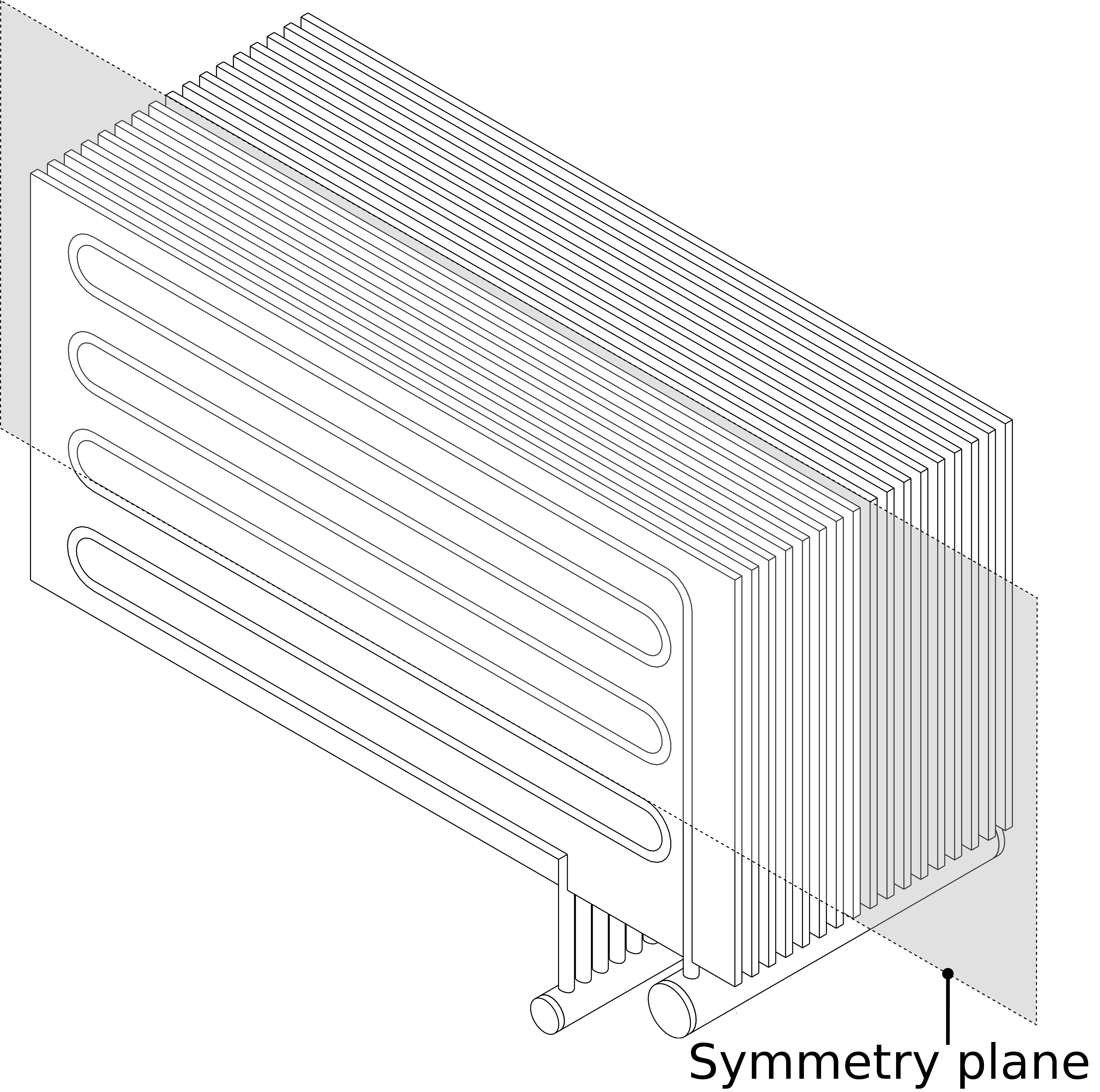
(b) Detail of the condenser and symmetry plane

Figure 2: Two-phase cooling system based on the thermosyphon principle experimental ; iecon11 .

This kind of device consists of an evaporator and a condenser connected by a pipe in which a mixture of liquid and vapor phases is flowing. The heat generated by an electronic device in contact with the evaporator is collected by means of an evaporating fluid. The vapor phase fluid, rising in the pipe, passes through the condenser where it returns to the liquid phase. As no pumps are needed to move the refrigerant fluid from the evaporator to the condenser, the resulting thermodynamical efficiency of two-phase cooling systems is remarkably superior to that of water-cooled or air-cooled systems (see Lasance1997 ). In order to deepen our understanding of the mechanisms that determine the performance of a two-phase thermosyphon cooler device and to facilitate the further optimization of its design, in the present research we focus on the study of the condenser subsystem (see Fig. 2(b)), for which we develop a multiscale mathematical model that is implemented in a numerical simulation code. As computational efficiency is a stringent requirement in industrial design and optimization procedures, model complexity is suitably reduced through the adoption of physically sound consistent assumptions that allow us to end up with a system of nonlinearly coupled 2D PDEs for the air and panel temperatures, and 1D PDEs for the refrigerant fluid flow.

Another important constraint is represented by the ability of the computational method to reproduce on the discrete level important physical features characterizing the problem at hand, such as mass and flux conservation, and its robustness in the presence of dominating convective flow regimes. These requirements are here satisfied by the introduction of a stabilized mixed finite element scheme on quadrilateral grids that automatically provides the desired inter-element flux conservation and upwinding through the use of suitable quadrature rules for the mass flux matrix and convection term. The resulting discrete method has also an immediate interpretation in terms of finite volume formulation which allows a compact implementation of the scheme that highly improves the overall efficiency of the computer-aided design procedure.

A final issue of critical importance in the development of a reliable computational tool for use in industrial design is model calibration and validation. Model calibration is properly addressed by supplying the parameter setting in the equation system with suitable empirical correlations, that are functional relations between two or more physical variables, usually obtained by means of a series of experimental tests. In common engineering practice, correlations are widely used because they allow to account for complex physical phenomena in a simple and synthetic manner, albeit their applicatibility is clearly restricted to a specific admissible range of parameter values. Model validation is carried out through extensive numerical simulations of the two-phase condenser under realistic working conditions.

An outline of the article is as follows. Sect. 2.1 describes the two–dimensional model for heat convection in air and heat diffusion in the panel whose derivation from the corresponding full 3D model is outlined in A. The simplified geometrical representation of the coolant–filled channel and the one–dimensional system of PDEs describing the flow within it are dealt with in Sect. 2.2. Sect. 3 discusses the decoupled iterative algorithm used to solve the complete model while Sects. 4 and 5 are devoted to the discussion of the discretization techniques adopted to treat each differential subsystems arising from system linearization. Finally, in Sect. 6 simulation results are presented and discussed and in Sect. 7 conclusions are drawn and possible future research directions are addressed.

2 Mathematical Models

In this section we describe the mathematical model on which our numerical simulation tool for the condenser is based. The equations for heat convection in air and heat diffusion in the panel wall are presented in Sect. 2.1, while the model for the two-phase flow in the channel is in Sect. 2.2.

2.1 2D model for the panel wall and air flow

The model for heat diffusion and convection is based on the following set of simplifying assumptions:

1. the geometry of the channel embedded into each panel of the condenser is the same;

2. air flow is in steady-state conditions;

3. air flow conditions in between each pair of condenser fins are identical;

4. air flow velocity $\boldsymbol{v}_{a}$ is everywhere parallel to the fin plates and its magnitude varies only in the orthogonal direction;

5. air density $\rho_{a}$ is constant;

6. the thickness of each panel is negligible compared to its size in any other direction;

7. the thickness of the air layer separating two panels in the condenser is negligible compared to the panel size in any other direction.

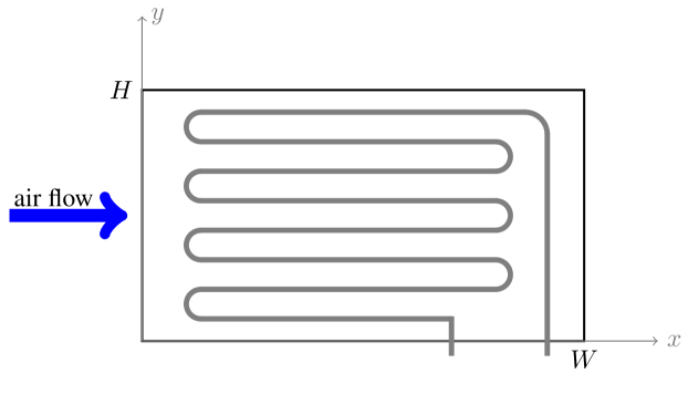
Figure 3: Computational domain for the two-dimensional heat flow problem.

Under the assumptions above, symmetry considerations lead to define the simplified computational domain $\Omega:=(0,W)\times(0,H)\subset\mathbb{R}^{2}$ illustrated in Fig. 3, in such a way that the air temperature $T_{a}$ and panel temperature $T_{w}$ satisfy in $\Omega$ the following equations which express conservation of energy:

$${\boldsymbol{\nabla}}\cdot(-k_{a}{\boldsymbol{\nabla}}T_{a}+\rho_{a}{c_{p}}\widetilde{\boldsymbol{v}}_{a}T_{a})+\widetilde{\textit{h}}_{aw}(T_{a}-T_{w})=0,$$ (1a)

$${\boldsymbol{\nabla}}\cdot(-k_{w}{\boldsymbol{\nabla}}T_{w})+\textit{h}_{aw}^{\ast}(T_{w}-T_{a})+\textit{h}_{wc}^{\ast}(T_{w}-T_{c})=0,$$ (1b)

complemented by the boundary conditions:

$$T_{a}={T_{a}}^{in} \quad y=0,$$ (1c)

$$-k_{a}{\boldsymbol{\nabla}}T_{a}\cdot\boldsymbol{n}=0 \quad y=H,$$ (1d)

$$(-k_{a}{\boldsymbol{\nabla}}T_{a}+\rho_{a}c_{p}\widetilde{\boldsymbol{v}}_{a}T_{a})\cdot\boldsymbol{n}=0 \quad x=0,\ x=W,$$ (1e)

$$-k_{w}{\boldsymbol{\nabla}}T_{w}\cdot\boldsymbol{n}=0 \quad y=0,\ y=H,\ x=0,\ x=W.$$ (1f)

The unknown functions $T_{a}=T_{a}(x,y)$ and $T_{w}=T_{w}(x,y)$ are the air and wall temperature respectively, $c_{p}$ is the air specific heat capacity at constant pressure and $k_{a}$ and $k_{w}$ are the thermal conductivities of air and panel material (e.g., aluminium), respectively. The function $T_{c}=T_{c}(x,y)$ represents the temperature of the cooling two-phase fluid in the channel network and is assumed to be a given datum in the solution of the equation system (1). The parameters $\widetilde{\textit{h}}_{aw}$ and $\textit{h}_{aw}^{\ast}$ are the heat transfer coefficient $\textit{h}_{aw}$ between air and condenser wall divided by suitably defined characteristic lengths $\lambda_{1a}$ and $\lambda_{1w}$, respectively. Precisely, $\lambda_{1a}$ is related to the variation of $k_{a}$ in the direction between air and condenser wall while $\lambda_{1w}$ is related to the variation of $k_{w}$ in the thickness of the condenser wall. The quantity $\textit{h}_{wc}^{\ast}$ is the heat exchange coefficient $\textit{h}_{wc}$ between the fluid and the panel wall divided by $\lambda_{1w}$. The vector field $\widetilde{\boldsymbol{v}}_{a}$ is the air flow velocity multiplied by the factor $\lambda_{2a}/\lambda_{1a}$ where $\lambda_{2a}$ is another characteristic length related to the formation of the thermal boundary layer at the interface between air and panel.

The quantities $W$ and $H$ are the size of the panel in the $x$ and $y$ directions, respectively, and $\boldsymbol{n}$ is the outward unit vector along the external surface of $\Omega$. It is important to notice that the physical properties of air, namely $k_{a}$ and $c_{p}$, as well as the panel material properties, e.g. $k_{w}$, and, when simulations are carried out in the natural convection regime, also the magnitude of the air velocity $\widetilde{\boldsymbol{v}}_{a}$, depend on the temperatures $T_{a}$ and $T_{w}$, hence problem (1) is nonlinear. The detailed derivation of (1) from the corresponding 3D model is illustrated for convenience in A.

2.2 Model for the channel subsystem

The channel embedded in each panel, where the two-phase coolant flows, is modeled as a pipeline network bandahertyklar ; BrouwerGasserHerty ; herty ; formaggia2012 , i.e., a set of a number $M$ of 1D straight pipe segments $\boldsymbol{\sigma}_{j}\subset\Omega,\ j=1,\ldots,M$. Such segments are joined at a set of $N$ vertices $\mathbf{x}_{i}\in\Omega,\ i=1,\ldots,N$ and each is parametrized by a (scalar) local coordinate $s_{j}$ such that $0\leq s_{j}\leq L_{j}$, $L_{j}$ being the length of $\boldsymbol{\sigma}_{j}$.

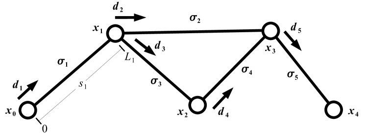
Figure 4: Example of channel network geometry and notation.

For each junction $\mathbf{x}_{i}$, we denote by $I^{-}_{i}\subseteq\{1,\ldots,N\}$, the set of those indices $j$ for which $\mathbf{x}_{i}$ is the first endpoint of the segment $\boldsymbol{\sigma}_{j}$, i.e., $j\in I^{-}_{i}\Leftrightarrow\mathbf{x}(s_{j})\big{|}_{s_{j}=0}=\mathbf{x}_{i}$, where $\mathbf{x}$ is the (vector) cartesian coordinate. Similarly, we define $I^{+}_{i}\subseteq\{1,\ldots,N\}$, to be the set of those indices $j$ for which $\mathbf{x}_{i}$ is the second endpoint of the segment $\boldsymbol{\sigma}_{j}$, i.e., $j\in I^{+}_{i}\Leftrightarrow\mathbf{x}(s_{j})\big{|}_{s_{j}=L_{j}}=\mathbf{x}_{i}$. We assume each parametrization to be uniform, i.e., $j\in I^{-}_{m}\cap I^{+}_{n}\Leftrightarrow\mathbf{x}(s_{j})=\mathbf{x}_{m}+\mathbf{d}_{j}s_{j}$, where $\mathbf{d}_{j}=(\mathbf{x}_{n}-\mathbf{x}_{m})/L_{j}$ is the unit vector defining the direction of $\boldsymbol{\sigma}_{j}$. Furthermore, we introduce the two additional vertices $\mathbf{x}_{0}$ and $\mathbf{x}_{N+1}$ representing the inlet and the outlet of the channel and we assume that they are connected to the first node of the first pipe and second node of the last pipe, respectively, so that we have $I^{-}_{0}\equiv\{1\}$, $I^{+}_{0}\equiv\varnothing$, $I^{-}_{N+1}\equiv\varnothing$ and $I^{+}_{N+1}\equiv\{M\}$.

Within each pipe $\boldsymbol{\sigma}_{j}$ we assume the following 1D equations, stating conservation of mass, momentum and energy, respectively, to hold (see, e.g., hermes2008numerical ):

$$\partial_{s_{j}}G_{j}=0,$$ (2a)

$$\partial_{s_{j}}\left(\displaystyle\frac{G_{j}^{2}}{\rho_{j}}+p_{j}\right)=f_{j}+\rho_{j}\mathbf{g}\cdot\mathbf{d}_{j},$$ (2b)

$$\partial_{s_{j}}\left(G_{j}\mathcal{H}_{j}\right)+\textit{h}_{wc}\left(T_{cj}-T_{w}\right)=0.$$ (2c)

where $G_{j}$, $\rho_{j}$, $p_{j}$, $f_{j}$, $\mathcal{H}_{j}$ and $T_{cj}$ are momentum, density, pressure, frictional forces, specific enthalpy and temperature of the two-phase fluid in each segment $\boldsymbol{\sigma}_{j}$, respectively, while $\mathbf{g}$ is the vector denoting the acceleration of gravity. In view of numerical discretization, it is convenient to rewrite equations (2a)- (2b) as:

$$\left\{\begin{array}[]{l}\partial_{s_{j}}G_{j}=0\\[5.69054pt] \partial_{s_{j}}\varphi_{j}=R_{j}G_{j}+\rho_{j}\mathbf{g}\cdot\mathbf{d}_{j}\end{array}\right.$$ (3)

where $\varphi_{j}=G_{j}^{2}/\rho_{j}+p_{j}$ denotes the total dynamical pressure and $R_{j}=f_{j}/G_{j}$ denotes the pipe hydraulic resistance per unit length. Similarly, equation (2c), upon introducing the symbol $\mathcal{W}_{j}$ denoting the enthalpy flux, can be rewritten as:

$$\left\{\begin{array}[]{l}\partial_{s_{j}}\mathcal{W}_{j}=h_{wc}(T_{w}-T_{cj})\\[5.69054pt] \mathcal{W}_{j}=G_{j}\mathcal{H}_{j}.\end{array}\right.$$ (4)

To close system (2), we need:

1. a set of coupling conditions at the $N$ junctions $\mathbf{x}_{i},\ i=1,\ldots,N$;

2. a set of boundary conditions at the inlet and outlet sections;

3. a set of constitutive relations.

All of these relations will be defined in the subsections below.

2.2.1 Coupling conditions

At each of the junction nodes $\mathbf{x}_{i}$ we impose the following coupling conditions, $\forall i\in\{1,\ldots,N\},\,\forall j\in I^{-}_{i},\,\forall k\in I^{+}_{i}$:

$$\left.\varphi_{j}\right|_{s_{j}=0}=\left.\left(\displaystyle\frac{G_{j}^{2}}{\rho_{j}}+p_{j}\right)\right|_{s_{j}=0}=\left.\left(\displaystyle\frac{G_{k}^{2}}{\rho_{k}}+p_{k}\right)\right|_{s_{k}=L{k}}=\left.\varphi_{k}\right|_{s_{k}=L{k}},$$ (5a)

$$\left.\mathcal{H}_{j}\right|_{s_{j}=0}=\left.\mathcal{H}_{k}\right|_{s_{k}=L{k}},$$ (5b)

$$\displaystyle\sum_{j}\left.-G_{j}\right|_{s_{j}=0}+\displaystyle\sum_{k}\left.G_{k}\right|_{s_{k}=L{k}}=0,$$ (5c)

$$\displaystyle\sum_{j}\left.-\mathcal{W}_{j}\right|_{s_{j}=0}+\displaystyle\sum_{k}\left.\mathcal{W}_{k}\right|_{s_{k}=L{k}}=\displaystyle\sum_{j}\left.-\left(G_{j}\mathcal{H}_{j}\right)\right|_{s_{j}=0}+\displaystyle\sum_{k}\left.\left(G_{k}\mathcal{H}_{k}\right)\right|_{s_{k}=L{k}}=0.$$ (5d)

These conditions express continuity of total dynamical pressure and enthalpy and conservation of mass and enthalpy fluxes at the junctions.

2.2.2 Boundary conditions

At the inlet $\mathbf{x}_{0}$ and outlet $\mathbf{x}_{N+1}$ we apply the following boundary conditions:

$$\varphi_{1}\Big{|}_{s_{1}=0}=\left(\displaystyle\frac{G_{1}^{2}}{\rho_{1}}+p_{1}\right)\Big{|}_{s_{1}=0}=p_{inlet},$$ (6a)

$$\mathcal{H}_{1}\Big{|}_{s_{1}=0}=\mathcal{H}_{inlet},$$ (6b)

$$G_{1}\Big{|}_{s_{1}=0}=G_{M}\Big{|}_{s_{M}=L_{M}}=G_{tot},$$ (6c)

where $p_{inlet}$, $\mathcal{H}_{inlet}$ and $G_{tot}$ are given data.

2.2.3 Constitutive relations

Within each pipe $\boldsymbol{\sigma}_{j}$ we assume the following constitutive relations, defining the homogeneous flow regime, to hold:

$$\rho_{j}=\displaystyle\frac{\rho_{V}(T_{cj})\rho_{L}(T_{cj})}{\rho_{V}(T_{cj})(1-\textit{x}_{j})+\rho_{L}(T_{cj})\textit{x}_{j}},$$ (7a)

$$\mathcal{H}_{j}=\mathcal{H}_{L}(T_{cj})(1-\textit{x}_{j})+\mathcal{H}_{V}(T_{cj})\textit{x}_{j},$$ (7b)

$$p_{j}=\textit{p}(T_{cj}).$$ (7c)

The two-phase density $\rho_{j}$ and enthalpy $\mathcal{H}_{j}$ are calculated through the empirical interpolation between all liquid flow (subscript $L$ in (7)) and all vapor flow quantities (subscript $V$ in (7)) that are weighted by the vapor quality $\textit{x}_{j}$. All the single-phase quantities depend implicitly on the temperature $T_{cj}$ of the two-phase fluid in the $j$-th segment $\boldsymbol{\sigma}_{j}$, hence system (7) is nonlinear. For a detailed description of the two-phase constitutive relations, we refer to collier1996convective , thome2006engineering and whalley1996two . After analyzing the review of the most recent correlation of the heat transfer coefficient for condensation inside tubes cavallini2003condensation and garcia2003review , we have decided to consider the Shah correlation shah1979general , valid for film condensation pattern, in the modified version proposed in (carichino2010, , Chap. 4). To model the frictional forces $f_{j}$ we used a relation based on the Blasius equation (thome2006engineering, , Chap. 13). For the dependence of the air velocity $\widetilde{\boldsymbol{v}}_{a}$ on the average temperature of the neighbouring panels and on the temperature of air at inflow we used correlations given in bar1984thermally .

3 Iterative Algorithms

The staggered algorithm used for the coupling of the different subsystems is depicted in the flow-chart of Fig. 5.

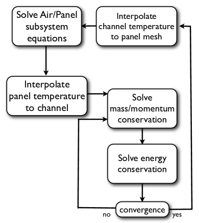
Figure 5: Schematic rapresentation of the staggered iteration algorithm.

The procedure consists of a nested fixed-point iteration composed of: 1) an outer iteration loop to solve the 2D air/panel subsystem; and 2) an inner iteration loop to solve the non-linear problems within each subsystem. In more detail, the outer iteration proceeds as follows:

1. Given $T_{c}$ and $\widetilde{h}_{aw}$, compute a new value for $T_{a}$ and $T_{w}$ by solving system (1).

2. Determine the value of $T_{w}$ at each node of the channel network.

3. Solve system (2) to update the quantities $G$, $\mathcal{H}$, $p$ describing the state of the fluid flow in the channel and, as a by-product, compute the fluid temperature $T_{c}$ and the vapor quality.

4. Go back to step 1.

Inner iteration loops are required to solve the non-linear heat flow equations at step 1. and for solving the nonlinear coupled system for the two phase flow at step 3. For the former we employ a monolithic quasi-Newton algorithm, while for the latter we further decouple the equations and proceed as follows:

1. Solve subsystem (2a)- (2b) to update $G$ and $p$.

2. Solve subsystem (2c) to update $\mathcal{H}$.

3. Determine the density, temperature and vapor quality using system (7).

4. Go back to step 3.1.

4 Dual Mixed-Finite Volume Discretization of the 2D Subproblems

In this section we describe the dual mixed-finite volume (MFV) method used for the numerical approximation of the air/panel physical model, presented in Sect. 2.1.

4.1 Dual mixed finite element approximation

Consistently with Sect. 2.1, we assume that the computational domain $\Omega$ is a rectangular open bounded set of $\mathbb{R}^{2}$ and denote by $\Gamma:=\partial\Omega$ and $\boldsymbol{n}$ the domain boundary and its outward unit normal vector, respectively. Then, we consider the following advection-diffusion-reaction model problem in mixed form:
find $u:\Omega\rightarrow\mathbb{R}$ and $\boldsymbol{J}:\Omega\rightarrow\mathbb{R}^{2}$ such that:

$$a\boldsymbol{J}+{\boldsymbol{\nabla}}u-a\boldsymbol{\beta}u=\boldsymbol{0} \qquad\mbox{in }\Omega,$$ (8a)

$$\nabla\cdot\boldsymbol{J}+\gamma u=f \qquad\mbox{in }\Omega,$$ (8b)

$$u=0 \qquad\mbox{on }\Gamma.$$ (8c)

In (8a), $a:=\alpha^{-1}$ is the inverse diffusion coefficient, with $\alpha>0$, and the convective field $\boldsymbol{\beta}$ is a given constant vector, while $f\in L^{2}(\Omega)$ and $\gamma\in L^{\infty}(\Omega)$ are given functions, with $\gamma(\boldsymbol{x})>0$. We also let $\boldsymbol{J}:=-\alpha{\boldsymbol{\nabla}}u+\boldsymbol{\beta}u$ be the flux associated with $u$, and we assume that (see douglasroberts1985 ; Arbogast_Chen95 )

$$\dfrac{\left\|{\boldsymbol{\beta}}\right\|_{L^{\infty}(\Omega)}}{4\,\alpha\,\displaystyle\inf_{\Omega}(\gamma)}<1.$$ (9)

Eq. (1a) is a special case of (8) upon setting $u:=T_{a}$, $\alpha:=k_{a}$, $\boldsymbol{\beta}:=\rho c_{p}\widetilde{\boldsymbol{v}}_{a}$, $\gamma:=\widetilde{h}_{aw}$ and $f:=\widetilde{h}_{aw}T_{w}$, with $T_{w}$ a known function, while Eq. (1b) is a special case of (8) upon setting $u:=T_{w}$, $\alpha:=k_{w}$, $\boldsymbol{\beta}:=\boldsymbol{0}$, $\gamma:=h_{aw}^{\ast}+h_{wc}^{\ast}$ and $f:=h_{aw}^{\ast}T_{a}+h_{wc}^{\ast}T_{c}$, with $T_{a}$ and $T_{c}$ known functions. Homogeneous Dirichlet boundary conditions for $u$ are assumed only for ease of presentation, because mixed and/or Neumann conditions can be easily handled by the proposed scheme (see sacco1997mixed ; BrezziMariniMichPietraSacco2006 ).

In view of the numerical approximation of (8), we introduce a regular decomposition $\mathcal{T}_{h}$ of $\Omega$ into ${\tt Nel}$ rectangles $K$ of area $|K|$ and center of gravity $\boldsymbol{x}_{G,K}$, and we denote by $\mathcal{E}_{h}$ the set of edges of $\mathcal{T}_{h}$ and by ${\tt Ned}$ the number of total edges of the mesh. We also let $\mathcal{E}_{h}^{in}$ denote the set of internal edges of $\mathcal{E}_{h}$. Let $\mathbb{P}_{k_{1},k_{2}}$ be the space of polynomials of degree less than or equal to $k_{1}$ with respect to $x$ and less than or equal to $k_{2}$ with respect to $y$. Let $k\geq 0$; for each $K\in\mathcal{T}_{h}$ we denote by $\mathbb{RT}_{[k]}(K):=\mathbb{P}_{k+1,k}(K)\times\mathbb{P}_{k,k+1}(K)$ the $k$-th order Raviart-Thomas (RT) mixed finite element space RaviartThomas1977 and by $\mathbb{Q}_{k}(K)=\mathbb{P}_{k,k}(K)$. We introduce the functional spaces $\mathbf{V}\equiv H_{{\rm div}}(\Omega)=\left\{\boldsymbol{v}:\boldsymbol{v}\in[L^{2}(\Omega)]^{2},\,\nabla\cdot\boldsymbol{v}\in L^{2}(\Omega)\right\}$ and $\mathbf{Q}\equiv L^{2}(\Omega)$, and their corresponding finite dimensional approximations:

$$\begin{array}[]{rcl}\mathbf{V}_{h}&=&\left\{\boldsymbol{v}_{h}\in\mathbf{V}:\ \boldsymbol{v}_{h}\big{|}_{K}\in\mathbb{RT}_{[0]}(K)\ \forall K\in\mathcal{T}_{h}\right\},\\ \mathbf{Q}_{h}&=&\left\{q_{h}\in\mathbf{Q}:\ q_{h}\big{|}_{K}\in\mathbb{Q}_{0}(K)\ \forall K\in\mathcal{T}_{h}\right\}.\end{array}$$

Functions in $\mathbf{V}_{h}$ are linear along each coordinate direction and discontinuous over $\mathcal{T}_{h}$ but have continuous normal component across each edge $e\in\mathcal{E}_{h}^{in}$. Functions in $Q_{h}$ are piecewise constant and discontinuous over $\mathcal{T}_{h}$.

To reflect the different nature of the degrees of freedom of functions in $\mathbf{V}_{h}$ and $\mathbf{Q}_{h}$, we introduce two different adjacency structures.

For each (oriented) edge $\boldsymbol{e}\in\mathcal{E}_{h}^{in}$, we indicate by $|\boldsymbol{e}|$ the length of $\boldsymbol{e}$, and we denote by $K^{+}_{e}$ and $K^{-}_{e}$ the pair of mesh elements such that $\boldsymbol{e}=\partial K^{+}_{e}\cap\partial K^{-}_{e}$. We also denote by $\boldsymbol{n}_{e}^{+}$ the unit normal vector on $\boldsymbol{e}$ pointing from $K^{+}_{e}$ to $K^{-}_{e}$ and define $\boldsymbol{n}_{e}^{-}=-\boldsymbol{n}_{e}^{+}$ as the unit normal vector to $\boldsymbol{e}$ pointing from $K^{-}_{e}$ to $K^{+}_{e}$. In the case where $\boldsymbol{e}\in\partial\Omega$, we set $\boldsymbol{n}_{e}^{+}:=\boldsymbol{n}$. We indicate by $d_{e}$ the distance between $\boldsymbol{x}_{G,K^{+}_{e}}$ and $\boldsymbol{x}_{G,K^{-}_{e}}$. In the case where $\boldsymbol{e}\in\Gamma$, $d_{e}$ is the distance between $\boldsymbol{x}_{G,K^{+}_{e}}$ and the midpoint of edge $\boldsymbol{e}$.

For each element $K\in\mathcal{T}_{h}$, we denote by $e(l)$, $l=1,\ldots,4$, the label number of edge $\boldsymbol{e}_{l}$, and by $K_{l}$ the mesh element neighbour of $K$ with respect to edge $\boldsymbol{e}_{l}$, whenever $\boldsymbol{e}_{l}$ does not belong to $\Gamma$. For any function $w_{h}\in\mathbf{Q}_{h}$, we introduce the two following operators associated with each edge of $\mathcal{E}_{h}^{in}$

$$\llbracket w_{h}\rrbracket_{e}:=w^{K^{+}_{e}}\boldsymbol{n}_{e}^{+}+w^{K^{-}_{e}}\boldsymbol{n}_{e}^{-},\qquad\{w_{h}\}_{e}:=\displaystyle\frac{1}{2}(w^{K^{+}_{e}}+w^{K^{-}_{e}}),$$

where for each $K\in\mathcal{T}_{h}$, $w^{K}$ is the constant value of $w_{h}$ over $K$. The operator $\llbracket w_{h}\rrbracket_{e}$ is the jump of $w_{h}$ across $\boldsymbol{e}$ while $\{w_{h}\}_{l}$ is the average of $w_{h}$ across $\boldsymbol{e}$. The previous definitions apply also in the case where $\boldsymbol{e}\in\partial{\Omega}$ by setting $w^{K^{-}_{e}}:=0$. Finally, let $\boldsymbol{v},\,\boldsymbol{w}$ be any pair of vectors in $(L^{2}(\Omega))^{2}$, and $v,\,w$ be any function pair in $L^{2}(\Omega)$. We set $A(\boldsymbol{v},\,\boldsymbol{w}):=\int_{\Omega}a\,\boldsymbol{v}\cdot\boldsymbol{w}$, $B(v,\,\boldsymbol{v}):=-\int_{\Omega}v\,\nabla\cdot\boldsymbol{v}$, $C(v,\,\boldsymbol{v}):=-\int_{\Omega}v\boldsymbol{\beta}\cdot\boldsymbol{v}$ and $(v,\,w):=\int_{\Omega}v\,w$.

Then, the dual mixed finite element approximation of (8) over quadrilateral grids reads: find $u_{h}\in\mathbf{Q}_{h}$ and $\boldsymbol{J}_{h}\in\mathbf{V}_{h}$ such that, for all $\boldsymbol{\tau}_{h}\in\mathbf{V}_{h}$ and for all $q_{h}\in\mathbf{Q}_{h}$, we have:

$$A(\boldsymbol{J}_{h},\boldsymbol{\tau}_{h})+B(u_{h},\boldsymbol{\tau}_{h})+C(u_{h},\boldsymbol{\tau}_{h})=0$$ (10a)

$$B(q_{h},\boldsymbol{J}_{h})-(q_{h},\gamma\,u_{h})=-(q_{h},f).$$ (10b)

Equation (10a) is the discretized form of the constitutive law (8a), while equation (10b) is the discretized form of the conservation law (8b). The finite element pair $\mathbf{Q}_{h}\times\mathbf{V}_{h}$ satisfies the inf-sup compatibility condition, so that problem (10), under the coerciveness assumption (9), admits a unique solution and optimal error estimates can be proved for the pair $(u_{h},\boldsymbol{J}_{h})$ in the appropriate graph norm (see RaviartThomas1977 ; BrezziFortin1991 ; Arbogast_Chen95 ). The DM formulation can be written in matrix form as

$$\left[\begin{array}[]{cc}\mathbf{A}&\quad(\mathbf{B}^{T}+\mathbf{C})\\ \mathbf{B}&\quad\mathbf{D}\end{array}\right]\,\left(\begin{array}[]{c}\mathbf{j}\\ \mathbf{u}\end{array}\right)=\left(\begin{array}[]{c}\mathbf{0}_{\tt Ned}\\ \mathbf{f}\end{array}\right)$$ (11)

where $\mathbf{A}\in\mathbb{R}^{{\tt Ned}\times{\tt Ned}}$ is the flux mass matrix, $\mathbf{B}\in\mathbb{R}^{{\tt Nel}\times{\tt Ned}}$, $\mathbf{C}\in\mathbb{R}^{{\tt Ned}\times{\tt Nel}}$ and $\mathbf{D}\in\mathbb{R}^{{\tt Nel}\times{\tt Nel}}$, while $\mathbf{u}\in\mathbb{R}^{{\tt Nel}\times 1}$, $\mathbf{j}\in\mathbb{R}^{{\tt Ned}\times 1}$ is the unknown vector pair, and $\mathbf{0}_{\tt Ned}$ is the column null vector of size Ned. Two computational difficulties are associated with the solution of the DM problem (10). The first difficulty is that the linear algebraic system (11) is in saddle-point form and has a considerably larger size than a standard displacement–based method of comparable order. The second difficulty is that, even in the particular case where $\boldsymbol{\beta}$ is equal to zero, it is not possible to ensure that the stiffness matrix acting on the sole variable $\mathbf{u}$ (obtained upon block Gaussian elimination) is an M-matrix for every value of $\gamma$ (see MariniPietra1989 in the case of triangular RT elements). This implies that the discrete maximum principle (DMP) can be satisfied by the DM method only if the mesh size $h$ is sufficiently small, and this constraint may become even more stringent if convection is present in the model.

4.2 The stabilized dual mixed finite volume approximation

To overcome the above mentioned difficulties, we introduce a (strongly consistent) modification of the DM method that extends to the case of quadrilateral grids the approach for triangular grids proposed and analyzed in sacco1997mixed ; BrezziMariniMichPietraSacco2006 . The introduced modifications consist of: 1) replacing the bilinear form $A(\boldsymbol{J}_{h},\boldsymbol{\tau}_{h})$ with the approximate bilinear form $A_{h}(\boldsymbol{J}_{h},\boldsymbol{\tau}_{h})$ obtained by using the trapezoidal quadrature formula; 2) replacing the bilinear form $C(u_{h},\boldsymbol{\tau}_{h})$ with $C_{h}(u_{h},\boldsymbol{\tau}_{h}):=C(\{u_{h}\},\boldsymbol{\tau}_{h})$; 3) adding to the left-hand side of (10a) the stabilization term

$$S(u_{h},\,\boldsymbol{\tau}_{h}):=-\displaystyle\sum_{\boldsymbol{e}\in\mathcal{E}_{h}^{in}}\varrho_{e}(\mathbb{P}e_{e})\displaystyle\int_{\boldsymbol{e}}\llbracket u_{h}\rrbracket_{e}\cdot\boldsymbol{\tau}_{h}\qquad\boldsymbol{\tau}_{h}\in\mathbf{V}_{h},$$ (12)

where $\mathbb{P}e_{e}:=(\left|{\boldsymbol{\beta}\cdot\boldsymbol{n}_{e}}\right|d_{e})/(2\alpha)$ is the local Pèclet number associated with edge $\boldsymbol{e}$ and $\varrho_{e}:\boldsymbol{e}\in\mathcal{E}_{h}\rightarrow\mathbb{R}^{+}$ is a stabilization function equivalent to adding, for each edge of $\mathcal{E}_{h}$, an artificial diffusion to the original problem.

The resulting stabilized DM formulation reads: find $u_{h}\in\mathbf{Q}_{h}$ and $\boldsymbol{J}_{h}\in\mathbf{V}_{h}$ such that, for all $\boldsymbol{\tau}_{h}\in\mathbf{V}_{h}$ and for all $q_{h}\in\mathbf{Q}_{h}$, we have:

$$A(\boldsymbol{J}_{h},\boldsymbol{\tau}_{h})+B(u_{h},\boldsymbol{\tau}_{h})+C_{h}(u_{h},\boldsymbol{\tau}_{h})+S(u_{h},\,\boldsymbol{\tau}_{h})=0$$ (13a)

$$B(q_{h},\boldsymbol{J}_{h})-(q_{h},\gamma\,u_{h})=-(q_{h},f).$$ (13b)

The significant advantage of introducing the modifications 1)–3) with respect to the standard DM approach is that, for each element $K\in\mathcal{T}_{h}$, the flux of $\boldsymbol{J}_{h}$ across the edge $e(l)$, $l=1,\ldots,4$ (the degree of freedom of $\boldsymbol{J}_{h}$), can be expressed explicitly as a function of the sole degrees of freedom $u^{K}$ and $u^{K_{l}}$ as

$$j_{e(l)}(u^{K},u^{K}_{l})=\left[-\alpha(1+\varrho_{e}(\mathbb{P}e_{e(l)}))\left(\dfrac{u^{K_{l}}-u^{K}}{d_{e(l)}}\right)+\boldsymbol{\beta}\cdot\boldsymbol{n}_{e(l)}\left(\dfrac{u^{K}+u^{K_{l}}}{2}\right)\right]|\boldsymbol{e}_{l}|.$$ (14)

Replacing the above expression into the discrete conservation law (13b), we end up with the stabilized dual mixed-finite volume (MFV) approximation of the model problem (8)

$$\left\{\begin{array}[]{ll}\displaystyle\sum_{l=1}^{4}j_{e(l)}(u^{K},u^{K_{l}})+u^{K}\overline{\gamma}_{K}|K|=\overline{f}_{K}|K|&\qquad\forall K\in\mathcal{T}_{h},\\[14.22636pt] u^{K_{l}}=0&\qquad\boldsymbol{e}_{l}\in\Gamma,\end{array}\right.$$ (15)

where $\overline{\gamma}_{K}$ and $\overline{f}_{K}$ are the mean values of $\gamma$ and $f$ on $K$, respectively. The above proposed stabilized MFV method is the extension to rectangular elements of the formulation for triangular grids introduced and analyzed in sacco1997mixed ; BrezziMariniMichPietraSacco2006 . For a similar use of numerical quadrature aimed to construct a finite volume variant of the DM method, we refer to vanNooyen in the case of the advection-diffusion-reaction model problem and to Fortin1995 for the approximate solution of the Stokes problem in fluid-dynamics.

The MFV method (15) can be written in matrix form as

$$\mathbf{K}\mathbf{u}=\mathbf{g}$$ (16)

where, for $K=1,\ldots,{\tt Nel}$, the entries of the stiffness matrix and of the load vector are:

$$\begin{array}[]{l}\mathbf{K}_{K,K}=\displaystyle\sum_{l=1}^{4}\left[\dfrac{\alpha(1+\varrho_{e}(\mathbb{P}e_{e(l)}))}{d_{l}}+\dfrac{\boldsymbol{\beta}\cdot\boldsymbol{n}_{e(l)}}{2}\right]|\boldsymbol{e}_{l}|+\overline{\gamma}_{K}|K|\\[11.38109pt] \mathbf{K}_{K,K_{l}}=\left[-\dfrac{\alpha(1+\varrho_{e}(\mathbb{P}e_{e(l)}))}{d_{l}}+\dfrac{\boldsymbol{\beta}\cdot\boldsymbol{n}_{e(l)}}{2}\right]|\boldsymbol{e}_{l}|\\[11.38109pt] \mathbf{g}_{K}=\overline{f}_{K}|K|.\end{array}$$ (17)

Matrix $\mathbf{K}$ is sparse and has at most four nonzero entries for each row, in the typical format of lowest-order finite volume methods. Proceeding along the same lines as in sacco1997mixed , we can prove the following result.

Proposition 1

Let the edge artificial viscosity $\varrho_{\boldsymbol{e}}(\mathbb{P}e_{\boldsymbol{e}})$ be chosen in such a way that

$$\varrho_{\boldsymbol{e}}(\mathbb{P}e_{\boldsymbol{e}})\geq\mathbb{P}e_{\boldsymbol{e}}-1\qquad\forall\boldsymbol{e}\in\mathcal{E}_{h}.$$ (18)

Then, $\mathbf{K}$ is an irreducible diagonally dominant M-matrix with respect to its colums Varga1962 .

As a consequence of Prop. 1, the MFV scheme (13) satisfies the DMP irrespective of the local convective term and mesh size. This lends the scheme a property of robustness which is a significant benefit in industrial computations like those considered in the present article. The simplest choice that allows to satisfy (18) is the upwind stabilization

$$\varrho_{l}(\mathbb{P}e_{\boldsymbol{e}})=\mathbb{P}e_{\boldsymbol{e}}\qquad\forall\boldsymbol{e}\in\mathcal{E}_{h}.$$ (19)

Another, more elaborate, choice is the so called Scharfetter-Gummel (SG) stabilization

$$\varrho_{l}(\mathbb{P}e_{\boldsymbol{e}})=\mathbb{P}e_{\boldsymbol{e}}-1+\mathcal{B}(2\mathbb{P}e_{\boldsymbol{e}})\qquad\forall\boldsymbol{e}\in\mathcal{E}_{h},$$ (20)

where $\mathcal{B}(x):=x/(e^{x}-1)$ is the inverse of the Bernoulli function. This latter choice is also known as exponential fitting ScharfetterGummel1969 ; RoosStynesTobiska1996 . The two above stabilizations tend to the same limit as the Pèclet number increases. However, their behaviour is quite different as the mesh size $h$ decreases, because (19) introduces an artificial diffusion of $\mathcal{O}(h)$ as $h\rightarrow 0$ while (20) introduces an artificial diffusion of $\mathcal{O}(h^{2})$ as $h\rightarrow 0$. For this reason, the SG stabilized MFV formulation is preferable as far as accuracy is concerned, and is the one implemented in the simulations reported in Sect. 6.

4.3 Numerical validation of the MFV discretization

In this section, we perform a numerical validation of the stabilized MFV method (13) applied to the solution of the model problem (8) with $\Omega=(0,1)\times(0,1)$.

In a first case study, we verify the convergence rate of the scheme when $\boldsymbol{\beta}=[0,\ 1]^{T}$, $\gamma=1$ and $f$ is computed in such a way that the exact solution is $u(x,y)=\cos x\sin y$. As for the diffusion coefficient, we choose $\alpha=\{1,10^{-1},10^{-2},10^{-3},10^{-4}\}$, in order to analyze both dominating diffusive and convective regimes. Computations are performed on increasingly refined grids of $N\times N$ square elements of dimension varying from $N=4$ to $N=64$. Fig. 6 shows the discrete maximum norm of the discretization error

$$\|u-u_{h}\|_{\infty,h}:=\max_{K\in\mathcal{T}_{h}}|u(\boldsymbol{x}_{G,K})-u^{K}|$$

as a function of $\alpha$ and of the mesh size $h=1/N$. Results indicate that for low values of the Pèclet number $\mathbb{P}e$, corresponding for example to $\alpha=1$, the SG method has a convergence order of $\mathcal{O}(h^{2})$, that decreases to $\mathcal{O}(h)$ for dominating convection regimes, as for $\alpha=10^{-4}$. On the other hand, the estimated convergence error of the upwind method is never better than $\mathcal{O}(h)$ for every value of $\alpha$.

(a) Upwind stabilization

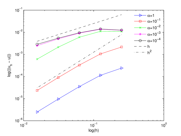
(b) SG stabilization

Figure 6: Logarithmic plot of the maximum norm of the discretization error as a function of $h$ and $\alpha$.

In a second case study, we validate the robustness and accuracy of the SG stabilization in the solution of the two numerical examples considered in xu1999monotone where $\alpha=10^{-6}$, $\gamma=0$ and $h=2^{-6}$. In the first example, $f=1$ and $\boldsymbol{\beta}=[-y,x]^{T}$. The scope of this computation is to verify the accuracy and stability of the method in managing a boundary layer without introducing spurious oscillations. In the second example, $f=0$ and $\boldsymbol{\beta}=\nabla\psi$, $\psi$ being the potential function defined as

$$\psi=\left\{\begin{array}[]{lrcl}0&0\leq&d+x&<0.55,\\ 2(d-0.55)&\quad 0.55\leq&d+x&<0.65,\\ 0.2&0.65\leq&d+x,&\end{array}\right.$$

where $d=(x^{2}+y^{2})^{1/2}$. Mixed Dirichlet-Robin conditions are enforced on the boundary $\Gamma$ in such a way that the solution exhibits two interior layers, one of which is very sharp. For graphical purposes, the computed values of $u_{h}$ have been interpolated through a nodally continuous function. Results reported in Fig. 7 are in excellent agreement with those of xu1999monotone and demonstrate the robustness of the stabilized MFV method with respect to dominating convective terms and its ability in capturing sharp boundary and interior layers without introducing any spurious oscillation in accordance with Prop. 1.

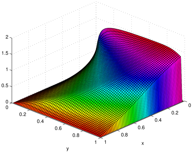
(a) Boundary layer example

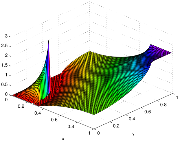
(b) Interior layer example

Figure 7: Surface plot of the numerical solution of two problems with sharp boundary and interior layers.

5 Primal Mixed Discretization of the 1D Fluid Equations

In this section we focus on the description of the Primal Mixed (PM) finite element scheme used for the discretization of the two-phase fluid equations (2) (see RobertsThomas1991 for an introduction to PM methods applied to the numerical solution of elliptic boundary value problems). In the following, we consider one pipe only and drop the subscript denoting the pipe being considered.

We start by noting that both (3) and (4) are special instances of the following boundary value problem to be solved in the 1D domain $\sigma=(0,L)$:

$$\partial_{s}J=f$$ (21a)

$$-\varepsilon\partial_{s}u+\beta u=J+g$$ (21b)

$$u(0)=u(L)=0$$ (21c)

where $f$, $\beta$ and $g$ are given data, and $\varepsilon$ is a non-negative diffusion coefficient. We recover (3) by setting $J=-G$, $u=\varphi$, $\varepsilon=R^{-1}$, $g=-R^{-1}\rho\mathbf{g}\cdot\mathbf{d}$, $f=0$ and $\beta=0$, while we recover (4) by setting $J=\mathcal{W}$, $u=\mathcal{H}$, $\varepsilon=0$, $g=0$, $f=h_{wc}(T_{w}-T_{c})$ and $\beta=G$.

Remark 1 (Hyperbolic character of the two-phase fluid model)

From the mathematical point of view, the model problem (21) represents an advective-diffusive model in conservation form quite similar to that introduced in Sect. 4 for the description of the air/panel physical model. In the present case, however, there is an important difference because the two-phase fluid equations (2) have an hyperbolic character so that the introduction of a diffusive term in the model system (21) must be regarded as a stabilization term for the corresponding numerical discretization of equations (2). For this reason, throughout the section, we always assume $\varepsilon$ to be strictly positive.

Remark 2 (Extension to pipeline geometry)

The advective-diffusive model (21) is here solved in the interval $\sigma=(0,L)$ only for ease of presentation of the Primal Mixed Finite Element Method approximation. The incorporation of the coupling conditions (5) at each junction node of the pipeline newtwork is straightforward with the adopted discretization scheme and is discussed in detail in the remainder of the section.

Let $\varepsilon$ be a positive bounded function and set $a:=\varepsilon^{-1}$. Then, the advective-diffusive problem (21) can be written in mixed form as:
find $u:\sigma\rightarrow\mathbb{R}$ and $J:\sigma\rightarrow\mathbb{R}$ such that:

$$aJ+\partial_{s}u-a\beta u+ag=0 \qquad\mbox{in }\sigma,$$ (22a)

$$\partial_{s}J=f \qquad\mbox{in }\sigma,$$ (22b)

$$u(0)=u(L)=0.$$ (22c)

We assume that

$$\partial_{s}(a\beta)\geq 0\qquad\mbox{a.e. in }\sigma.$$ (23)

In view of the numerical approximation of (22) we introduce a partition $\mathcal{T}_{h}$ of $\sigma$ into $N$ intervals $K_{i}$ of length $h_{i}$, $i=1\ldots N$, by means of $N+1$ nodes $s_{j},j=0\ldots N,s_{0}=0,s_{N}=L$. We also introduce the following function spaces defined on $\mathcal{T}_{h}$:

$$\begin{array}[]{l}V_{h}=\left\{v_{h}\in C^{0}(\overline{\sigma}):v_{h}|_{K_{i}}\in\mathbb{P}_{1}(K)\,\forall K\in\mathcal{T}_{h},\,v_{h}(0)=v_{h}(L)=0\right\}\\[5.69054pt] Q_{h}=\left\{p_{h}\in L^{2}(\sigma):p_{h}|_{K_{i}}\in\mathbb{P}_{0}(K)\,\forall K\in\mathcal{T}_{h}\right\}.\end{array}$$ (24)

Functions in $V_{h}$ are piecewise linear continuous over $\overline{\sigma}$ and vanish at the boundary $\partial\sigma$ while functions in $Q_{h}$ are piecewise constant over $\sigma$. Nodal continuity of functions in $V_{h}$ ensures the automatic satisfaction of the coupling conditions (5a) and (5b).

The PM finite element approximation of (22) reads:
find $u_{h}\in V_{h}$ and $J_{h}\in Q_{h}$ such that:

$$A(J_{h},q_{h})+B(u_{h},q_{h})+C(u_{h},q_{h})=-(ag,q_{h}) \qquad\forall q_{h}\in Q_{h}$$ (25a)

$$B(v_{h},J_{h})=-(v_{h},f) \qquad\forall v_{h}\in V_{h},$$ (25b)

where

$$\begin{array}[]{l}A(J_{h},q_{h}):=\displaystyle\int_{\sigma}a\,J_{h}\,q_{h}\,ds,\\[11.38109pt] B(v_{h},J_{h}):=\displaystyle\int_{\sigma}J_{h}\,\partial_{s}v_{h}\,ds,\\ C(u_{h},q_{h}):=\displaystyle-\int_{\sigma}a\,\beta\,u_{h}\,q_{h}\,ds\end{array}$$

and $(\cdot,\cdot)$ denotes the scalar product in $L^{2}(\sigma)$. It can be checked that under the coercivity assumption (23), problem (25) is uniquely solvable.

The PM system (25) can be written in matrix form as

$$\left[\begin{array}[]{cc}\mathbf{A}&\quad(\mathbf{B}^{T}+\mathbf{C})\\ \mathbf{B}&\mathbf{0}\end{array}\right]\,\left(\begin{array}[]{c}\mathbf{j}\\ \mathbf{u}\end{array}\right)=\left(\begin{array}[]{c}\mathbf{g}\\ \mathbf{f}\end{array}\right)$$ (26)

where $\mathbf{A}\in\mathbb{R}^{N\times N}$ is the flux mass matrix, $\mathbf{B}\in\mathbb{R}^{(N-1)\times N}$ and $\mathbf{C}\in\mathbb{R}^{N\times(N-1)}$, while $\mathbf{u}\in\mathbb{R}^{(N-1)\times 1}$, $\mathbf{j}\in\mathbb{R}^{N\times 1}$ is the unknown vector pair, and $\mathbf{0}\in\mathbb{R}^{(N-1)\times(N-1)}$ is the null square matrix of size $N-1$. Compared with the dual mixed system (11), the PM formulation (26) has a considerable advantage because matrix $\mathbf{A}$ is diagonal, each diagonal entry $A_{kk}$ corresponding to the element $K_{k}$ in the grid, $k=1,\ldots,N$. Assuming that $\varepsilon$, $\beta$ and $g$ are constant over each element $K_{i}$, the first equation of (25) can be solved for the flux $J_{h}$ over each mesh element

$$J_{k}=-\varepsilon_{k}\displaystyle\frac{u_{k}-u_{k-1}}{h_{k}}+\beta_{k}\displaystyle\frac{u_{k-1}+u_{k}}{2}-g_{k}\qquad\forall i=k,\ldots,N.$$ (27)

Taking $v_{h}$ equal to the ”hat” function $\varphi_{i}$, equal to 1 at every internal node $s_{i}$ and zero at every other node, $i=1,\ldots,N-1$, we end up with the following system of nodal conservation laws:

$$J_{i+1}-J_{i}=f_{i}\left(\displaystyle\frac{h_{i}+h_{i+1}}{2}\right)\qquad i=1,\ldots,N-1.$$ (28)

The above equation expresses the fact that at each internal node of the partition the output flux $J_{i+1}$ is equal to the sum of the input flux $J_{i}$ plus the nodal production term $P_{i}:=f_{i}(h_{i}+h_{i+1})/2$, in strong analogy with the classical Kirchhoff law for the current in an electric circuit. In particular, if $f=0$, we get strong flux conservation at the node $s_{i}$, $i=1,\ldots,N-1$, which corresponds to enforcing in strong form the coupling conditions (5c) and (5d).

Substituting (27) into (28) we end up with the linear algebraic system in the sole variable $u_{h}$

$$\mathbf{M}\mathbf{U}=\mathbf{F}$$ (29)

where $\mathbf{U}\in\mathbb{R}^{(N-1)\times 1}$ is the vector of nodal dofs for $u_{h}$, $\mathbf{F}\in\mathbb{R}^{(N-1)\times 1}$ is the right-hand side and $\mathbf{M}\in\mathbb{R}^{(N-1)\times(N-1)}$ is the stiffness matrix whose entries are given by:

$$M_{ij}=\left\{\begin{array}[]{ll}-\displaystyle\frac{\varepsilon_{i}}{h_{i}}-\displaystyle\frac{\beta_{i+1}}{2}&\qquad j=i-1\\[5.69054pt] \displaystyle\frac{\varepsilon_{i}}{h_{i}}+\displaystyle\frac{\varepsilon_{i+1}}{h_{i+1}}+\displaystyle\frac{\beta_{i+1}}{2}-\displaystyle\frac{\beta_{i}}{2}&\qquad j=i\\[8.53581pt] -\displaystyle\frac{\varepsilon_{i+1}}{h_{i+1}}+\displaystyle\frac{\beta_{i+1}}{2}&\qquad j=i+1.\end{array}\right.$$

As in the case of the dual mixed method of Sect. 4.1, the matrix $\mathbf{M}$ turns out to be an M-matrix only if the mesh size $h$ is sufficiently small. To avoid this inconvenience, we define the local Pèclet number

$$\mathbb{P}e_{i}:=\displaystyle\frac{|\beta_{i}|h_{i}}{2\varepsilon_{i}}\qquad i=1,\ldots,N$$

and modify the PM finite element scheme by simply replacing in the first equation of (25) the term $a=\varepsilon^{-1}$ with

$$a_{h}|_{K_{i}}:=\left(\varepsilon_{i}(1+\mathbb{P}e_{i})\right)^{-1}=\left(\varepsilon_{i}+\displaystyle\frac{|\beta_{i}|h_{i}}{2}\right)^{-1}\qquad i=1,\ldots,N.$$

This amounts to adding a stabilizing artificial diffusion term of upwind type (cf. (19)) into the method and transforms system (29) into the stabilized PM scheme

$$\mathbf{M}^{stab}\mathbf{U}=\mathbf{F}$$ (30)

where the entries of the stiffness matrix $\mathbf{M}^{stab}$ of the stabilized PM method now read:

$$M_{ij}^{stab}=\left\{\begin{array}[]{ll}-\displaystyle\frac{\varepsilon_{i}}{h_{i}}-\beta_{i}^{+}&\qquad j=i-1\\[5.69054pt] \displaystyle\frac{\varepsilon_{i}}{h_{i}}+\displaystyle\frac{\varepsilon_{i+1}}{h_{i+1}}+\beta_{i+1}^{+}-\beta_{i}^{-}&\qquad j=i\\[8.53581pt] -\displaystyle\frac{\varepsilon_{i+1}}{h_{i+1}}+\beta_{i+1}^{-}&\qquad j=i+1\end{array}\right.$$

having set:

$$\begin{array}[]{ll}\beta^{+}:=\displaystyle\frac{\beta+|\beta|}{2}&\qquad(\geq 0)\\ \beta^{-}:=\displaystyle\frac{\beta-|\beta|}{2}&\qquad(\leq 0).\end{array}$$

By inspection on the expressions of $M_{ij}^{stab}$ we have the following result.

Proposition 2

The stiffness matrix $\mathbf{M}^{stab}$ is an irreducible diagonally dominant M-matrix with respect to its colums.

As in the case of the MFV scheme, Prop. 2 implies that the upwind stabilized PM finite element scheme satisfies the DMP. Moreover, the upwind PM method is at most first-order accurate with respect to the discretization parameter $h$.

Remark 3 (Stabilization method)

In the case of problem (4) the SG stabilization (20) cannot be used because $\varepsilon=0$. Therefore, to ensure a consistent treatment that is applicable in both hyperbolic and advective-diffusive regimes, the artificial diffusion term of upwind type (19) is added in the numerical examples of Sect. 5.1 and of Sect. 6.

5.1 Numerical validation of the PM discretization

In this section, we perform a numerical validation of the stabilized PM method (25) applied to the solution of the model problem (21) on the test network geometry depicted in Fig. 8.

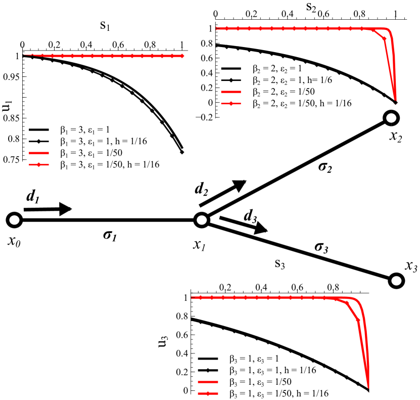
Figure 8: Test case on a three-segment network. Solid lines denote the exact solution while dotted lines denote the numerical solution computed by the upwind stabilized PM method.

In the first test case we study a diffusion-dominated flow while in the second test case the flow is in the advection-dominated regime. For both cases we let $\beta|_{\boldsymbol{\sigma}_{1}}=3$, $\beta|_{\boldsymbol{\sigma}_{2}}=2$, $\beta|_{\boldsymbol{\sigma}_{3}}=1$ and $f=g=0$. For the first test case, whose exact solution is shown in black in Fig. 8, we let $\varepsilon=1$ on all network segments, while for the second test, whose exact solution is shown in red in Fig. 8, we let $\varepsilon=1/50$. It is easily verified that the exact solution of both tests can be expressed as:

$$u(s)|_{\boldsymbol{\sigma}_{i}} =u(0)|_{\boldsymbol{\sigma}_{i}}\displaystyle\frac{e^{\displaystyle(\beta|_{\boldsymbol{\sigma}_{i}}L_{i})/\varepsilon}-e^{\displaystyle(\beta|_{\boldsymbol{\sigma}_{i}}s)/\varepsilon}}{e^{\displaystyle(\beta|_{\boldsymbol{\sigma}_{i}}L_{i})/\varepsilon}-1}+u(L_{i})|_{\boldsymbol{\sigma}_{i}}\displaystyle\frac{e^{\displaystyle(\beta|_{\boldsymbol{\sigma}_{i}}s)/\varepsilon}-1}{e^{\displaystyle(\beta|_{\boldsymbol{\sigma}_{i}}L_{i})/\varepsilon}-1}$$ (31a)

$$J(s)|_{\boldsymbol{\sigma}_{i}} =\beta|_{\boldsymbol{\sigma}_{i}}\displaystyle\frac{u(0)|_{\boldsymbol{\sigma}_{i}}e^{\displaystyle(\beta|_{\boldsymbol{\sigma}_{i}}L_{i})/\varepsilon}-u(L_{i})|_{\boldsymbol{\sigma}_{i}}}{e^{\displaystyle(\beta|_{\boldsymbol{\sigma}_{i}}L_{i})/\varepsilon}-1}$$ (31b)

for $i=1,2,3$, where $L_{1}=L_{2}=L_{3}=1$, $u(0)|_{\boldsymbol{\sigma}_{1}}=1$, $u(L_{1})|_{\boldsymbol{\sigma}_{1}}=u(0)|_{\boldsymbol{\sigma}_{2}}=u(0)|_{\boldsymbol{\sigma}_{3}}=\omega$ and $u(L_{2})|_{\boldsymbol{\sigma}_{2}}=u(L_{3})|_{\boldsymbol{\sigma}_{3}}=0$. The value $\omega$ of the solution $u$ at the junction node $x_{1}$ is determined from the flux continuity condition

$$J|_{\boldsymbol{\sigma}_{1}}=J|_{\boldsymbol{\sigma}_{2}}+J|_{\boldsymbol{\sigma}_{3}},$$

that yields

$$\omega=\displaystyle\frac{\frac{\varepsilon}{L_{1}}\mathcal{B}\left(\frac{-\beta|_{\boldsymbol{\sigma}_{1}}L_{1}}{\epsilon}\right)u(0)|_{\boldsymbol{\sigma}_{1}}+\frac{\varepsilon}{L_{2}}\mathcal{B}\left(\frac{\beta|_{\boldsymbol{\sigma}_{2}}L_{2}}{\epsilon}\right)u(L_{2})|_{\boldsymbol{\sigma}_{2}}+\frac{\varepsilon}{L_{3}}\mathcal{B}\left(\frac{\beta|_{\boldsymbol{\sigma}_{3}}L_{3}}{\epsilon}\right)u(L_{3})|_{\boldsymbol{\sigma}_{3}}}{\frac{\varepsilon}{L_{1}}\mathcal{B}\left(\frac{\beta|_{\boldsymbol{\sigma}_{1}}L_{1}}{\epsilon}\right)+\frac{\varepsilon}{L_{2}}\mathcal{B}\left(\frac{-\beta|_{\boldsymbol{\sigma}_{2}}L_{2}}{\epsilon}\right)+\frac{\varepsilon}{L_{3}}\mathcal{B}\left(\frac{-\beta|_{\boldsymbol{\sigma}_{3}}L_{3}}{\epsilon}\right)}$$

where $\mathcal{B}$ is the inverse of the Bernoulli function introduced in Sect. 4.2.

Fig. 9 shows the logarithmic plots of the discretization errors $\|u-u_{h}\|_{V}$ and $\|J-J_{h}\|_{Q}$ as a function of the discretization parameter $h$ in the diffusive-dominated regime. The scheme turns out to have a first-order accuracy. This result confirms the validity of the error analysis carried out in RobertsThomas1991 in the case of a purely diffusive problem also in the case of an advective-diffusive model.

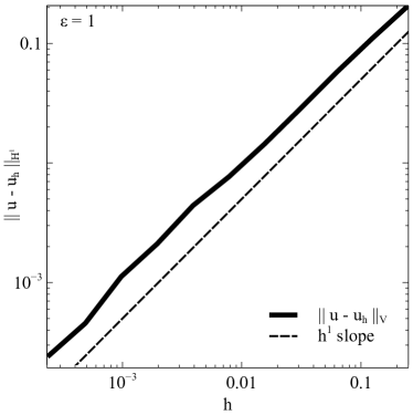
(a) $\|u-u_{h}\|_{V}$

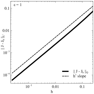
(b) $\|J-J_{h}\|_{Q}$

Figure 9: Logarithmic plot of the discretization error as a function of $h$ in the case $\varepsilon=1$.

Fig. 10 shows the logarithmic plots of the discretization errors $\|u-u_{h}\|_{V}$ and $\|J-J_{h}\|_{Q}$ as a function of the discretization parameter $h$ in the advective-dominated regime. The scheme is still first-order accurate with respect to $h$ in the computation of the primal variable $u$ despite the fact that the magnitude of the computed error is higher than in the diffusion-dominated regime. The reported error curve for the flux variable $J$ is dominated by the effect of round-off, in accordance with the fact that in the advective-dominated regime the flow is almost hyperbolic and the computed flux $J_{h}$ is a very good approximation of the exact flux $J$.

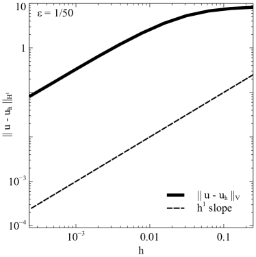
(a) $\|u-u_{h}\|_{V}$

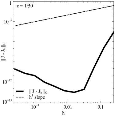
(b) $\|J-J_{h}\|_{Q}$

Figure 10: Logarithmic plot of the discretization error as a function of $h$ in the case $\varepsilon=1/50$.

We conclude the validation analysis of the upwind stabilized PM method by considering again Fig. 8 which shows the numerical solution of the benchmark problem (denoted by black and red dotted curves) computed with a grid spacing $h=1/16$ and superposed to the exact solution (31a). It is to be noted that in the advective-dominated regime ($\varepsilon=1/50$) the numerical solution almost coincides with the exact one in the first branch of the network $\sigma_{1}$ because there the problem is almost hyperbolic and the input datum $u(0)=1$ is transported by the fluid velocity. We also note that in the other two branches of the network, $\sigma_{2}$ and $\sigma_{3}$, even though the chosen stepsize is not sufficiently small to fully resolve the boundary layer at the outlets, the PM upwind method provides a solution which is monotone and free of spurious oscillations in accordance with Prop. 2. A more considerable error occurs in the computed solution when the problem is diffusion-dominated ($\varepsilon=1$) in accordance with the fact that the PM is only first-order accurate.

6 Simulation Results

In this section we perform a thorough validation of the computational model illustrated in the previous sections. The simulations are representative of realistic geometries of advanced cooling systems for power electronics. In particular aluminum condenser panels, as part of a two-phase thermosyphon loop, are simulated in natural convection operation mode. In Sect. 6.1 we analyze the impact of channel geometry and topology on the cooling performance, while in Sect. 6.2 we compare the model predictions with the measured data reported in iecon11 and based on the experimental campaign and methodology illustrated in experimental .

6.1 Comparison of different channel geometries

In this section we use our simulation code to estimate the impact of different pipe geometries on the cooling properties of the system. With this aim, we consider three test cases where panel size and material, input power, air velocity and temperature are the same, but with different channel paths.

The developed code represents a strong tool in the design of complex channel geometries allowing the researchers to optimize the topology of complex systems.

The simulation data are summarized in Tab. 1.

Parameter	Value	Units
$S$	$0.05$	m
$\lambda_{1}=\lambda_{2}$	$0.025$	m
$T_{a}^{in}$	$298.15$	K
$|\boldsymbol{V}_{a}^{in}|$	$1$	${\rm m}\,{\rm s}^{-1}$
$W$	$0.45$	m
$H$	$0.2$	m
$T_{0}$	$358.15$	K
$G_{tot}$	$5.8$	${\rm Kg}\,{\rm m}^{-2}\,{\rm s}^{-1}$
$h_{wc}$	$3$	${\rm W}\,{\rm m}^{-2}\,{\rm K}^{-1}$
$h_{aw}$	$1.1$	${\rm W}\,{\rm m}^{-2}\,{\rm K}^{-1}$

Table 1: Model parameters.

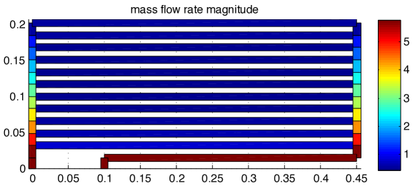
(a) device A

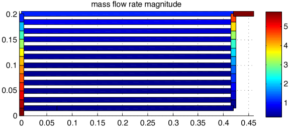
(b) device B

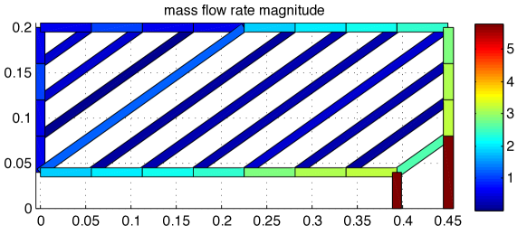
(c) device C

Figure 11: Comparison of mass flow rate magnitude for the three devices geometries.

The mass flux of coolant is the input datum of the simulation. Such value represents the total mass flowing through the panel, assuming the coolant to be in full vapor state at the inlet of the system.

The geometry of the three devices is compared in Fig. 11, with the color scale representing the absolute value of the mass flow rate in each channel segment.

The structure of a condenser panel is based on a series of parallel channels. A good flow distribution is a mandatory element for an optimal design, allowing the designer to maximally exploit the system and therefore increasing the maximum power density of the cooling device. Case ”a” and case ”b” indicate a better distribution of mass flow over the parallelized channels compared to case ”c”. Starting from case ”a” and ”b”, we see that the flow distribution is a function of the flow-path resistance: the higher the flow-path resistances, the lower is the flow rate. For case ”a”, the flow rate is higher in the lower channels, closer to the inlet, and slightly decreases toward the top part of the panel. The configuration ”b” is a possible design solution to overcome the pressure drop unbalance that may occur among the channels, and to guarantee a more uniform distribution over the entire surface due to equal inlet-outlet channel-flow-path length. Unfortunately, this effect is not present and a distribution of the mass flow rate similar to that in case ”a” is obtained. Case ”c” is studied to take advantage of the channel orientation and the positive effect of the gravitational field in the condensation process.

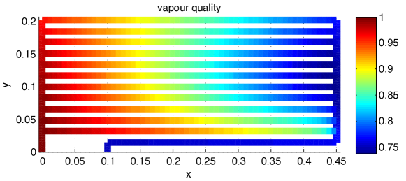
(a) device A

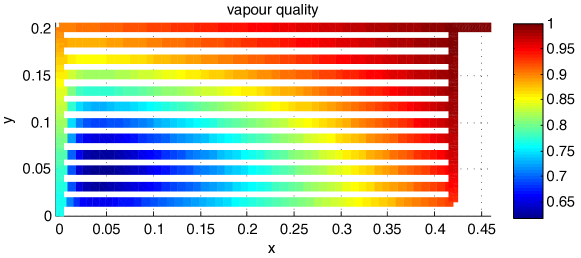
(b) device B

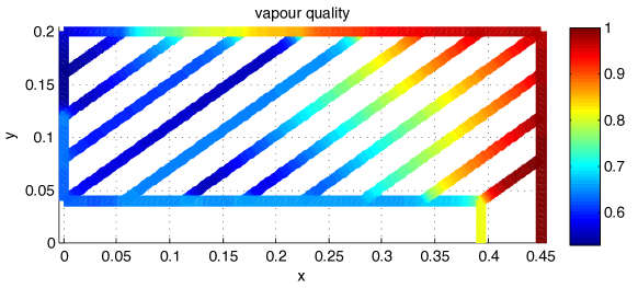
(c) device C

Figure 12: Comparison of vapor quality for the three devices geometries.

While the effect of gravity due to channel orientation helps reducing the pressure losses across the system, the short channels close to the flow inlet act as short circuit path, allowing high mass flow rates of vapor directly from inlet to outlet. This has the clear disadvantage that high flow rates of vapor cannot condense efficiently over a short distance. The described mass flow rate distribution has a strong effect on the local vapor quality, as depicted in Fig. 12. Generally, for a channel of fixed length, high flow rates correspond to a high vapor quality at the discharge. This phenomenon is particularly evident in case ”c”, where the lower sub-channel with the higher flow rate does not provide a good condensation due to its short length. The designer should seek for a balanced distribution of the vapor qualities at the discharge of each channel in order to exploit best the heat transfer area.

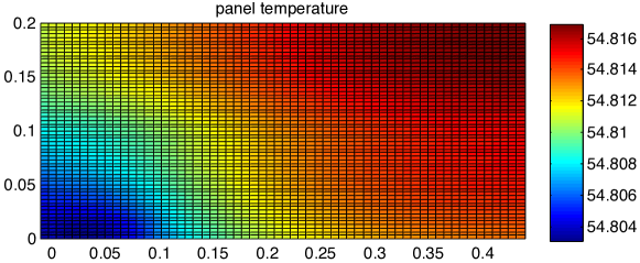
(a) device A

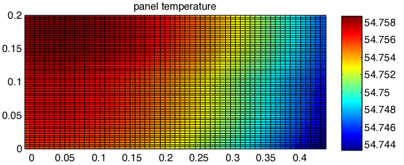
(b) device B

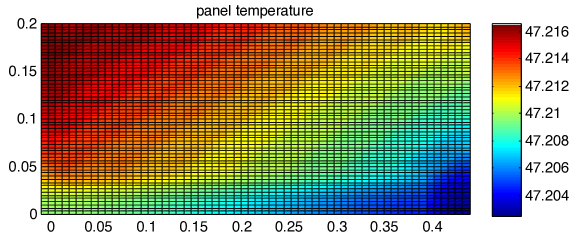
(c) device C

Figure 13: Comparison of panel temperature for the three device geometries.

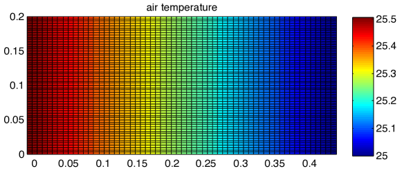
(a) device A

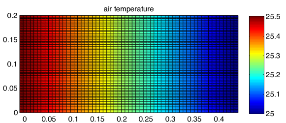
(b) device B

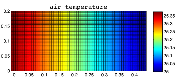
(c) device C

Figure 14: Comparison of air temperature for the three device geometries.

Fig. 13 shows the value of the panel temperature for the three different geometries. Results indicate an almost constant temperature distribution. This is characteristic of a two-phase system where the condensation heat transfer coefficients are orders of magnitude higher than those of the air side. Fig. 14 shows the evolution of the air temperature for the three different geometries. This plot is a good representation of the total heat transferred by the panel, representing the sensible heating of the air stream. Considering the original boundary condition of a fixed inlet mass flow rate of vapor, a higher air temperature difference indicates a higher amount of transferred heat. While case ”a” and case ”b” are comparable, case ”c” shows a lower air temperature at the discharge of the panel, clearly indicating a lower heat transfer to the air. This is well supported by the mass flow rate distribution and vapor quality plots. We also can notice that in Fig. 14 the air temperature differences are smaller in case ”c” compared to ”a” and ”b”. This is probably to be ascribed to the fact that a mass flux is enforced as boundary condition in the simulation model (mass flow rate of vapor per unit area) and not power.

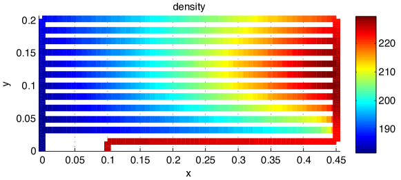
(a) device A

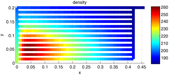
(b) device B

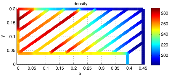
(c) device C

Figure 15: Comparison of the density of the two phase fluid for the three device geometries.

Fig. 15 shows the spatial distribution of the so called two phase density or bulk density for the three different device geometries. This quantity represents a weighted density between liquid and vapor densities, the weighting factor being the vapor quality. This means that the bulk density is the sum of the vapor and liquid densities multiplied by the vapor quality (vapor phase fraction) and its complement (liquid phase fraction), respectively. As a result, portions of the channels with higher bulk densities represent a fluid in a state with a higher content of liquid phase. To interpret Fig. 15 we can directly refer to Fig. 12, so that high flow rates imply a high vapor quality at the discharge and relatively low two phase densities. As discussed for Fig. 12, this latter phenomenon is particularly evident in case ”c” where the lower sub-channel with the higher flow rate does not provide a good condensation due to its short length and low vapor densities occur. As for the vapor quality, the design should seek for a balanced distribution of the two phase densities at the discharge of each channel in order to exploit at the best the heat transfer area and in order to have a balanced distribution of the liquid and vapor phases across the condensing panel.

6.2 Comparison with measured data

In this section we carry out a set of simulation runs to validate the performance of the computational model on realistic geometries and fluid-dynamical data. The experimental campaign and test set-up used for the validation follows closely what is presented in experimental and iecon11 . As described in iecon11 , the investigated cooling system is a thermosyphon device constituted of: an evaporator body, a vapor riser, a condenser (stack of roll-bonded panels) and a liquid downcomer. The evaporator can accommodate two ABB HighpakTM power semiconductor modules. Once the modules are in operation the evaporator collects the heat transferred by means of an evaporating fluid. The evaporator is designed in such a way that at its discharge the liquid is separated from the vapor. The liquid is brought back to the evaporator inlet while the vapor travels toward the condenser through the vapor riser. At the inlet of the condenser a vapor distributor feeds the stack of aluminum panels, equally distributing the mass flow among them. The panels are so-called roll-bonded panels, constituted of two aluminum sheets bounded together over almost the entire surface. Where this bounding is not present, a channel is generated, allowing the passage of the two-phase flow. The heat is rejected to the ambient by means of natural convection, the vapor is brought back to liquid conditions. Finally, the liquid is driven back to the evaporator inlet by gravity. The same aluminum panels and stack geometrical layout as presented in iecon11 is the subject of the investigation. The condenser is a stack of 13 panels 500 mm wide and 250 mm high, 1.2 mm thick, and equally spaced with a pitch of 18mm. Each panel contains 11 horizontal flow channels of a nominal length of 390 mm. The flow channel is formed on both sides of the panel with isoscele trapezoidal sections, the base and the height measuring 10 mm and 2.1 mm, respectively. The vapor and liquid phases are distributed to and collected from the panels by means of collectors of 19 and 16 mm internal diameter, respectively. Detailed drawings are available in iecon11 , while a detailed description of the experimental measurement techniques is presented in experimental . The experimental conditions are summarized in Tab. 2.

Fluid	R245fa
Refrigerant charge	2 Kg
Filling ratio	0.5
Heat Load	200 - 1600 W
Ambient temperature	298.15 K
Air cooling regime	Natural convection

Table 2: Experimental conditions.

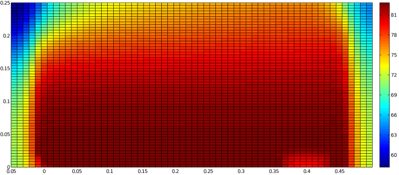
Figure 16: Computed panel temperature for a total dissipated power of $1500$ W.

Figure 16 presents the computed panel temperature corresponding to a power inflow of 1500 W, air inlet temperature of 25 ^∘C and natural convection operation. It is observed that the panel is almost isothermal. This is characteristic of the investigated system. A condensing fluid in the panel channels is characterized by high heat transfer coefficients, orders of magnitude higher than heat transfer coefficients typical of natural convection in air. The heat transfer conditions as well as the nature of the panel, sufficient thickness, small distance between channels and relatively high thermal conductivity of the aluminum result in an almost constant panel temperature. An almost constant temperature of the condenser panel is what we are looking for from an application point of view. It allows to overcome a common drawback of a standard heat-sink based system, where the metallic fin does not behave as a perfect fin (constant temperature) but has a temperature gradient from base to tip, resulting in a limited efficiency. Having an almost constant temperature results in an efficiency of the fin close to unity. The panel border is the coldest part. The low temperature in this region is is due to boundary effects. While the rest of the panel has an almost constant temperature, we can still identify a hotter region in the lower part of the panel compared to the top part.

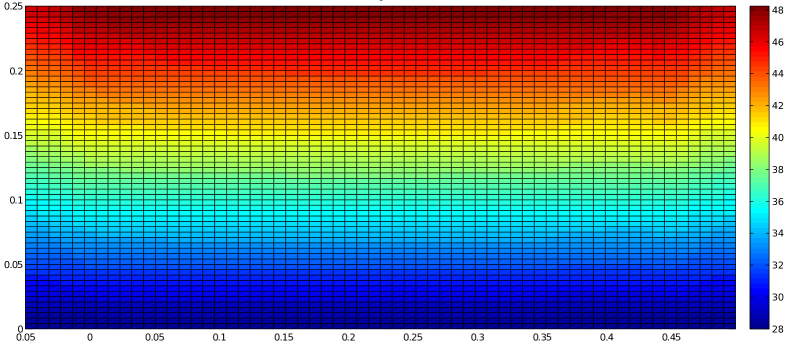
Figure 17: Computed air temperature for a total dissipated power of $1500$ W.

Figure 17 depicts the air temperature between two panels. The values are averaged in the direction perpendicular to the panel surface. The temperature pattern is characteristic of the transfer of sensible heat from panel to air in natural-convection operation. The large temperature difference between inlet and outlet of the condenser panel results from the small air velocity typical of natural convection. The maximum allowed temperature difference between inlet and outlet is usually a design parameter, and the designer of the device tries to optimize the system in order to match this value. A higher allowed temperature difference makes it possible to shrink the size of the device. On the other hand, when required, a decrease of the maximum temperature difference can be obtained by increasing the number of panels or the panel area. Since the panel temperature decreases from bottom to top, while the air temperature increases in that direction, the temperature difference between air and panel is largest at the panel bottom. This means that the heat flux from panel to air is maximum at the panel bottom.

The mass flow rate distribution among the panel channels plays an important role in the behavior of the condenser. During operation, the two-phase fluid tends to flow in the horizontal channels suitably paralleled. Considering the fact that the flow path through the panel and hence the flow resistance is smallest for the bottom channel, a decrease in mass flow rate from bottom to top is expected. A certain inhomogeneity in mass flow rate must therefore always be accounted for in the type of parallel connection of channels. Due to the higher mass flow rate, and consequently higher velocity in the bottom channel, a lower fluid residence time per channel length results. Consequently, it is expected that a longer channel length is needed to complete condensation.

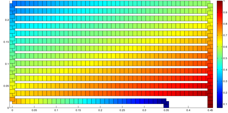
Figure 18: Computed refrigerant vapor quality for a total dissipated power of $1500$ W.

This is indeed observed in the simulation results in Figure 18, showing the local vapor quality in the channels. For the bottom channel, a longer distance from the channel inlet is needed for the vapor quality to decay to a certain value. Consequently, the vapor quality at the channel end, i.e. at the left in the figure, is highest for the bottom channel and lowest for the top channel. Furthermore, from the energy balance, it is clear the condensation of the highest mass flow rate in the bottom channel requires the largest heat flow rate from channel to air. Since all channels have the same surface area, one expects the heat flux to be highest for the bottom channel and lowest for the top channel. This closely agrees with the observation of maximum temperature difference between panel and air at the bottom and the corresponding maximum heat flux between panel and air in this region.

The designer may try to minimize the observed differences in performance between the condenser channels by optimizing the channel design. For example, one may try to achieve the same vapor quality at the end of all condenser channels. Complete condensation and hence low vapor quality is fundamental to guarantee a safe and reliable operation of the device, since a re-wetting of the evaporator surface is mandatory. It is exactly this kind of optimization tasks for which the present mathematical model is beneficial, as it provides insight in the detailed performance and behavior of the cooling device.

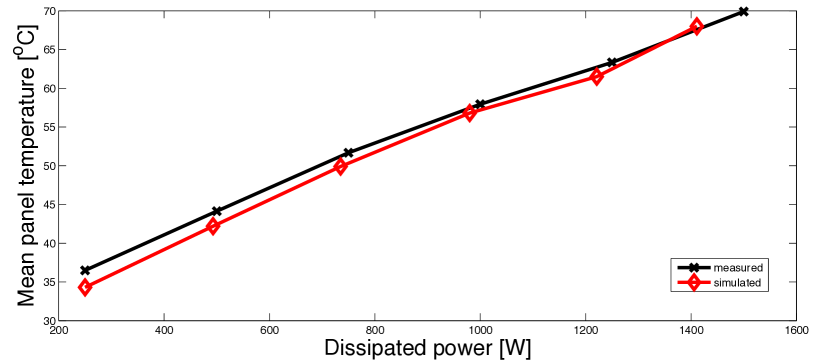
Figure 19: Average panel temperature (computed vs. measured) as a function of the total dissipated power.

Figure 19 shows a plot of the mean temperature of the panel as a function of the dissipated power. While the computed temperature distribution describes in great detail the operation of the device, the mean panel temperature is a synthetic parameter for the designer to validate in an immediate manner the predictive capabilities of the code. Agreement of numerical results of Figure 19 with experimental data is striking and indicates that, although based on many simplifying assumptions, our model does have very good predictive accuracy.

7 Conclusions and Future Work

In this article we have proposed and numerically implemented a multiscale thermo-fluid mathematical model for the description of a condenser component of a novel two-phase thermosyphon cooling system presented in experimental ; iecon11 . The condenser consists of a set of roll-bonded vertically mounted fins among which air flows by either natural or forced convection and plays an important role in the industrial design of advanced power electronics systems.

The mathematical model is developed with the aim of deepening the understanding of the various thermo-fluid mechanisms that determine the performance of the condenser in view of a further optimization of the cooling device. The adopted approach is based on a multiscale formulation meant to reduce as much as possible the complexity required by a fully three-dimensional (3D) simulation code while maintaining reasonable predictive accuracy.

More specifically, the flow of the two-phase coolant within the condenser fins is modeled as a 1D network of pipes, while heat diffusion in the fins and its convective transport in the air slab are modeled as 2D processes. The resulting mathematical problem consists of a system of nonlinearly coupled PDEs in conservation form that are characterized by a mixed parabolic-hyperbolic character with possible presence of strongly advective dominating terms. A fixed point iterative map is used to reduce the computational effort to the successive solution of a sequence of decoupled linear stationary boundary value problems in the 1D channel pipe network and in the 2D air domain, respectively.

For the numerical approximation of the above differential problems a Primal Mixed Finite Element discretization method with upwind stabilization is used for the 1D coolant flow while a Dual Mixed-Finite Volume scheme with Exponential Fitting stabilization is used for 2D heat diffusion and convection.

Extensive numerical tests are carried out to validate the stability and accuracy of the proposed schemes on several benchmark problems whose solution is characterized by the presence of steep interior and boundary layers. The obtained results confirm the good accuracy of the proposed formulation and its ability in satisfying a discrete maximum principle. This latter property confers robustness to the simulation tool and makes it suitable for heavy duty use in industrial applications.

The solver is then thouroughly applied to the numerical study and parametric characterization of a two-phase coolant system with realistic industrial geometry. The output of the simulations provide a complete map of the principal thermal and fluid dynamical variables of the problem (air temperature, coolant fluid pressure and vapor quality) that are extensively used by the project engineer to quantitavely design a novel device structure. Two groups of simulations are performed for the validation of the computational algorithm. In a first set of runs, the code is used to analyze the impact of channel geometry on the distribution of mass flow rate, vapor quality and panel temperature. In a second set of runs, the simulated average panel temperature of a given realistic cooler geometry is compared with available experimental data. Despite the several simplifying model assumptions introduced in the condenser mathematical description, the obtained results turn out to be in very good agreement with measures thus providing a sound indication of model reliability.

Even if applied to a problem arising in a specific area of thermo-fluid dynamical industrial applications, the multiscale modeling approach proposed in the present work can be used to study problems arising in other scientific contexts. For example, the computational model to couple 2D heat convection-diffusion and 1D flow in a pipeline network shares a close resemblance with the mathematical and numerical treatment of flow and mass transport in biological tissues that has been recently investigated in dAngelo2007 ; Shipley2010 ; Erbertseder2012 and references cited therein. This interesting similarity might be profitably used to apply to these latter novel bio-technological applications solution methods that in this article are proved to enjoy properties of accuracy, stability and conservation.

Further research activity will be devoted to the:

• topological optimization of the channels layout;

• integration of the condenser model in a complete thermosyphon loop simulation tool including evaporator body and connections;

• analysis of the existence of a fixed point of the iterative map and its possible uniqueness.

Appendix A Dimensionality Reduction of the Heat Convection-Diffusion Equations

In this section we illustrate the model reduction procedure that allows to derive under the assumptions (H1)–(H7) of Sect. 2.1 the simplified 2D model (1) from the corresponding 3-dimensional equations for heat convection and diffusion in the condenser walls and in the air between two plate walls. In order to describe the dimensionality reduction procedure, we start from the following model problem set in the 3D computational domain $\Omega$ depicted in Fig. 20:

$$\begin{array}[]{rcll}\nabla\cdot\left(-k{\boldsymbol{\nabla}}u+\rho c\boldsymbol{v}u\right)&=&0&\qquad\mbox{in }\Omega\\[8.53581pt] u&=&u_{in}&\qquad\mbox{on }\Sigma_{in}\\[8.53581pt] -k{\boldsymbol{\nabla}}u\cdot\boldsymbol{n}&=&0&\qquad\mbox{on }\Sigma_{out}\\[8.53581pt] \left(-k{\boldsymbol{\nabla}}u+\rho c\boldsymbol{v}u\right)\cdot{\boldsymbol{n}}&=&\textit{h}\ (u-u_{w})&\qquad\mbox{on }\Sigma_{w}\\[8.53581pt] \left(-k{\boldsymbol{\nabla}}u+\rho c\boldsymbol{v}u\right)\cdot\boldsymbol{n}&=&0&\qquad\mbox{on }\Sigma_{lat}\end{array}$$ (32)

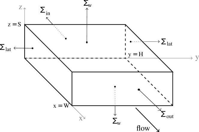
Figure 20: Three-dimensional domain for the heat convection-diffusion model problem.

We notice that the model problem (32) may describe either the forced heat convection between two fins or the heat diffusion in one fin wall. Referring to Fig. 20, in the latter case, we have $\Sigma_{in}=\Sigma_{out}=\varnothing$, $\boldsymbol{v}=\boldsymbol{0}$ and $\Sigma_{lat}=\displaystyle\cup_{i=1}^{4}\Sigma_{i}$, while in the former case we have $\Sigma_{in}=\Sigma_{1}$, $\Sigma_{out}=\Sigma_{3}$ and $\Sigma_{lat}=\Sigma_{2}\cup\Sigma_{4}$. The contact walls $\Sigma_{w}$, located at $z=0$ and $z=S$ respectively, represent the boundaries where heat exchange occurs. According to assumption (H4), the convection velocity $\boldsymbol{v}$ is directed along the $x$ axis, so that it can be expressed as

$$\boldsymbol{v}(z)=\boldsymbol{V}\ B(z)$$ (33)

where $\boldsymbol{V}$ is a constant vector directed along the $x$ axis and $B(z)$ is a dimensionless scalar shape function accounting for the velocity boundary layer in the $z$ direction.

The unknown function $u=u(x,y,z)$ represents a temperature (either air temperature or wall temperature), $\rho$ is the density of the medium contained in the domain $\Omega$, $c$ is the specific heat capacity of the medium and $k$ is its thermal conductivity.

Temperature is fixed at the inlet surface $\Sigma_{in}$ to a given value $u_{in}$. On the contact surfaces $\Sigma_{w}$ the outflow heat flux is proportional to the difference between temperature $u$ and the wall temperature $u_{w}$, through the heat transfer coefficient h. $\boldsymbol{n}$ is the outward unit vector along the external surface of the domain.

According to assumptions (H1) and (H3), the conditions at the upper and lower contact surface $\Sigma_{w}$ are symmetric. Therefore, we can define an adiabatic plane at $z=S/2$ which allows us to consider only the portion of space between the adiabatic surface and one of the two contacts $\Sigma_{w}$, for example that located at $z=0$.

We start our dimensionality reduction procedure by assuming the following ansatz for the unknown $u$

$$u(x,y,z)=U(x,y)\,Z(z),$$ (34)

where $U=U(x,y)$ expresses temperature variation in the $xy$ plane, while $Z=Z(z)$ is a dimensionless shape function accounting for temperature variation between the contact surface and the adiabatic plane located at $z=S/2$. The separated variable form of temperature distribution (34) agrees well with assumptions (H6) and (H7) according to which a mild variation of temperature between two neighbouring contact surfaces is to be expected. The next step consists in examining the dependence of problem coefficients on the unknown $u$. The heat capacity $c$ can be taken as a constant wassermann1966 . The same holds for the density $\rho$ (cf. assumption (H5)). As far as the thermal conductivity $k$, the following power law can be used wassermann1966

$$k(x,y,z)=k_{0}\left(\displaystyle\frac{u(x,y,z)}{u_{0}}\right)^{\beta}=k_{0}\left(\displaystyle\frac{U(x,y)Z(z)}{u_{0}}\right)^{\beta}$$ (35)

where $k_{0}$, $u_{0}$ and $\beta$ are suitable constants.

Integration of the balance equation in the vertical direction and the use of (33), (34) and (35) yield

$$\lambda_{1}{\boldsymbol{\nabla}}_{xy}\cdot\left(-k_{0}\left(\displaystyle\frac{U}{u_{0}}\right)^{\beta}{\boldsymbol{\nabla}}_{xy}U\right)+\lambda_{2}{\boldsymbol{\nabla}}_{xy}\cdot\left(\rho c\boldsymbol{V}U\right)+\mathbb{I}=0$$ (36)

where

$$\lambda_{1}:=\displaystyle\int_{0}^{S/2}Z^{\beta+1}(z)\ dz,\qquad\lambda_{2}:=\displaystyle\int_{0}^{S/2}Z(z)\ B(z)\ dz$$ (37)

and

$$\mathbb{I}:=\displaystyle\int_{0}^{S/2}\partial_{z}\left(-k\partial_{z}u\right)dz,$$

while ${\boldsymbol{\nabla}}_{xy}(\cdot)$ is the gradient operator with respect to the directions $x$ and $y$ only, The quantity $\lambda_{1}$ modulates the variation of thermal conductivity in the $z$ direction while the quantity $\lambda_{2}$ is related to the shape of the thermal boundary layer arising at the interface between air and panel. Using Gauss theorem to treat the quantity $\mathbb{I}$ we get

$$\mathbb{I}=\left[-k\partial_{z}u\right]_{0}^{S/2}=-\left(-k\left.\partial_{z}u\right|_{z=0}\right)$$

because $-k\left.\partial_{z}u\right|_{z=S/2}=0$ under the assumption of adiabatic surface, so that we can rewrite condition (32)₄ as

$$\textit{h}\left(u|_{z=0}-u_{w}\right)=(-k{\boldsymbol{\nabla}}u+\rho cu\boldsymbol{v})\cdot\boldsymbol{n}\Big{|}_{\Sigma_{w}}=-k{\boldsymbol{\nabla}}u\cdot\boldsymbol{n}\Big{|}_{\Sigma_{w}}=-\left(-k\partial_{z}u|_{z=0}\right)=\mathbb{I}.$$

Therefore, upon rescaling the shape function $Z$ in such a way that $Z(0)=1$, equation (36) becomes

$$\lambda_{1}{\boldsymbol{\nabla}}_{xy}\cdot\left(-k_{xy}{\boldsymbol{\nabla}}_{xy}U\right)+\lambda_{2}{\boldsymbol{\nabla}}_{xy}\cdot\left(\rho c\boldsymbol{V}U\right)+\textit{h}\left(U-u_{w}\right)=0$$

where we have defined the heat conductivity in the $xy$ plane (contact surface)

$$k_{xy}:=k_{0}\left(\displaystyle\frac{U(x,y)}{u_{0}}\right)^{\beta}=k_{0}\left(\displaystyle\frac{U(x,y)Z(0)}{u_{0}}\right)^{\beta}=k(x,y,0).$$

To end up with a 2D reduced model for heat convection and diffusion, we need specify the exponent $\beta$. At low pressures we typically have $\beta=0.9$ wassermann1966 so that $k$ is approximately a linear function of temperature. This latter quantity is used as a fitting parameter in the numerical simulations reported in Sect. 6. Thus, omitting the subscript $xy$ in the notation, and writing $u$ instead of $U$, the reduced 2D version of (32) reads:

$$\left\{\begin{array}[]{rcll}{\boldsymbol{\nabla}}\cdot(-k{\boldsymbol{\nabla}}u+\rho{c}\widehat{\boldsymbol{v}}u)+\widehat{\textit{h}}(u-u_{w})&=&0&\quad(x,y)\in\Omega,\\ u&=&u_{in}&\quad x=0,\\ -k{\boldsymbol{\nabla}}u\cdot\boldsymbol{n}&=&0&\quad x=W,\\ (-k{\boldsymbol{\nabla}}u+\rho c\widehat{\boldsymbol{v}}u)\cdot\boldsymbol{n}&=&0&\quad y=0,\ y=H,\end{array}\right.$$ (38)

where $\Omega:=(0,W)\times(0,H)$, $\widehat{\textit{h}}:=\textit{h}/\lambda_{1}$, $\widehat{\lambda}:=\lambda_{2}/\lambda_{1}$ and $\widehat{\boldsymbol{v}}:=\widehat{\lambda}\boldsymbol{V}$. Notice that the two heat balance equations (1a) and (1b) are special instances of (38) upon setting $u=T_{a}$, $k=k_{a}$, $\rho=\rho_{a}$, $c=c_{p}$, $\widehat{\boldsymbol{v}}=\widetilde{\boldsymbol{v}}_{a}$, $\widehat{\textit{h}}=\widetilde{\textit{h}}_{aw}$ and $u_{w}=T_{w}$ in the case of the air temperature model, and $u=T_{w}$, $k=k_{w}$, $\widehat{\boldsymbol{v}}=\boldsymbol{0}$, $\widehat{\textit{h}}={\textit{h}}_{aw}^{\ast}+\textit{h}_{wc}^{\ast}$, and $u_{w}=(\textit{h}_{aw}^{\ast}T_{a}+\textit{h}_{wc}^{\ast}T_{c})/(\textit{h}_{aw}^{\ast}+\textit{h}_{wc}^{\ast})$ in the case of the panel temperature model, respectively.

References

- [1] F. Agostini and T. Gradinger. Roll-bond condenser in a two-phase thermosyphon loop for power electronics cooling. In D. Poljak B. Sunden, C.A. Brebbia, editor, Advanced Computational Methods and Experiments in Heat Transfer XII, volume 75 of Transactions of the Wessex Institute collection. the Wessex Institute, 2012.
- [2] F. Agostini, T. Gradinger, and C. de Falco. Simulation aided design of a two-phase thermosyphon for power electronics cooling. In IECON 2011-37th Annual Conference on IEEE Industrial Electronics Society, pages 1560–1565. IEEE, 2011.
- [3] T. Arbogast and Z. Chen. On the implementation of mixed methods as nonconforming methods for second-order elliptic problems. Math. Comp., 64(211):943–972, 1995.
- [4] M. K. Banda, M. Herty, and A. Klar. Gas flow in pipeline networks. Networks and Heterogeneous Media, 1(1), March 2006.
- [5] A. Bar-Cohen and WM Rohsenow. Thermally optimum spacing of vertical, natural convection cooled, parallel plates. Journal of Heat Transfer, 106:116, 1984.
- [6] F. Brezzi and M. Fortin. Mixed and Hybrid Finite Element Methods. Springer Verlag, New York, 1991.
- [7] F. Brezzi, L.D. Marini, S. Micheletti, P. Pietra, and R. Sacco. Stability and Error Analysis of Mixed Finite Volume Methods for Advective-Diffusive Problems. Comput. Math. Appl., 51:681–696, 2006.
- [8] J. Brouwer, I. Gasser, and M. Herty. Gas pipeline models revisited: Model hierarchies, nonisothermal models, and simulations of networks. Multiscale Model. Simul., 9(2):601–623, 2011.
- [9] L. Carichino. Computational Models for Power Electronics Cooling Systems. Master’s thesis, Politecnico di Milano, 2010.
- [10] A. Cavallini, G. Censi, D. Del Col, L. Doretti, GA Longo, L. Rossetto, and C. Zilio. Condensation inside and outside smooth and enhanced tubes–a review of recent research. International Journal of Refrigeration, 26(4):373–392, 2003.
- [11] J.G. Collier and J.R. Thome. Convective boiling and condensation. Oxford University Press, USA, 1996.
- [12] C. d’Angelo. Multiscale modelling of metabolism and transport phenomena in living tissues. Phd dissertation, EPFL, 2007.
- [13] J. Jr. Douglas and J. E. Roberts. Global estimates for mixed method for second order elliptic equa-tions. Math. Comput., 44(169):39–52, 1985.
- [14] K. Erbertseder, J. Reichold, B. Flemisch, P. Jenny, and R. Helmig. A coupled discrete/continuum model for describing cancer-therapeutic transport in the lung. PLoS ONE, 7(3):e31966, 2012.
- [15] M. Farhloul and M. Fortin. A mixed finite element for the Stokes problem using quadrilateral elements. Advances in Computational Mathematics, 3:101–113, 1995.
- [16] L. Formaggia, A. Fumagalli, A. Scotti, and P. Ruffo. A reduced model for Darcy’s problem in networks of fractures. Technical Report MOX-Report No. 32/2012, MOX, Dipartimento di Matematica ”F. Brioschi”, Politecnico di Milano, P.zza L. da Vinci 32 - 20133 Milano, Italy, 2012.
- [17] O. Garcia-Valladares. Review of in-tube condensation heat transfer correlations for smooth and microfin tubes. Heat Transfer Engineering, 24(4):6–24, 2003.
- [18] C.J.L. Hermes, C. Melo, and C.O.R. Negrao. A numerical simulation model for plate-type, roll-bond evaporators. International Journal of Refrigeration, 31(2):335–347, 2008.
- [19] M. Herty. Coupling conditions for networked systems of Euler equations∗. Siam J. Sci. Comput., 30(3):1596–1612, 2008.
- [20] C. Lasance. Technical data column. Electronics Cooling, 1997.
- [21] L.D. Marini and P. Pietra. An Abstract Theory for Mixed Approximations of Second Order Elliptic Problems. Mat. Aplic. Comput., 8:219–239, 1989.
- [22] P.A. Raviart and J.M. Thomas. A mixed finite element method for second order elliptic problems. In I. Galligani and E. Magenes, editors, Mathematical Aspects of Finite Element Methods,I. Springer-Verlag, Berlin, 1977.
- [23] J.E. Roberts and J.M. Thomas. Mixed and hybrid methods. In P.G. Ciarlet and J.L. Lions, editors, Finite Element Methods, Part I. North-Holland, Amsterdam, 1991. Vol.2.
- [24] H. G. Roos, M. Stynes, and L. Tobiska. Numerical methods for singularly perturbed differential equations. Springer-Verlag, Berlin Heidelberg, 1996.
- [25] R. Sacco and F. Saleri. Stabilized mixed finite volume methods for convection-diffusion problems. East-West Journal of Numerical Mathematics, 5(4):291–311, 1997.
- [26] D.L. Scharfetter and H.K. Gummel. Large signal analysis of a silicon Read diode oscillator. IEEE Trans. Electron Devices, ED-16:64–77, 1969.
- [27] M.M. Shah. A general correlation for heat transfer during film condensation inside pipes. International Journal of Heat and Mass Transfer, 22(4):547–556, 1979.
- [28] R.J. Shipley and S.J. Chapman. Multiscale modelling of fluid and drug transport in vascular tumours. Bulletin of Mathematical Biology, 72(6):1464–1491, 2010.
- [29] J.R. Thome. Engineering Data Book III. Wolverine Tube, Inc, 2006.
- [30] R.R.P. van Nooyen. A Petrov-Galerkin mixed finite element method with exponential fitting. Numer. Meth. Part. Differ., 11(5):501–524, 1995.
- [31] R.S. Varga. Matrix Iterative Analysis. Englewood Cliffs, New Jersey, 1962.
- [32] A.A. Wasserman, Ya.Z. Kazavchinskiy, and V.A. Rabinovich. Thermophysical Properties of Air and Its Components. Science, Moscow,, 1966.
- [33] P.Bb Whalley. Two-phase flow and heat transfer. Oxford University Press Oxford, 1996.
- [34] J. Xu and L. Zikatanov. A monotone finite element scheme for convection-diffusion equations. Mathematics of Computation, 68(228):1429–1446, 1999.