Analysis of blue-shifted emission peaks in type II supernovae

Abstract

In classical P-Cygni profiles, theory predicts emission to peak at zero rest velocity. However, supernova spectra exhibit emission that is generally blue shifted. While this characteristic has been reported in many supernovae, it is rarely discussed in any detail. Here we present an analysis of H$\alpha$ emission-peaks using a dataset of 95 type II supernovae, quantifying their strength and time evolution. Using a post-explosion time of 30 d, we observe a systematic blueshift of H$\alpha$ emission, with a mean value of –2000 km s^-1. This offset is greatest at early times but vanishes as supernovae become nebular. Simulations of Dessart et al. (2013) match the observed behaviour, reproducing both its strength and evolution in time. Such blueshifts are a fundamental feature of supernova spectra as they are intimately tied to the density distribution of ejecta, which falls more rapidly than in stellar winds. This steeper density structure causes line emission/absorption to be much more confined; it also exacerbates the occultation of the receding part of the ejecta, biasing line emission to the blue for a distant observer. We conclude that blue-shifted emission-peak offsets of several thousand km s^-1 are a generic property of observations, confirmed by models, of photospheric-phase type II supernovae.

1 Introduction

Type II supernovae (SNe II henceforth) are classified through the presence of hydrogen Balmer lines in their spectra (see Minkowski 1941 for initial spectral classification of SNe, and Filippenko 1997 for a review). Spectral line formation occurring in optically thick, rapidly expanding ejecta produce spectral features to appear with a P-Cygni profile morphology. An observed P-Cygni profile is characterised by an absorption feature which is blueshifted, and an emission feature found closer to zero rest velocity. The blue-shifted absorption feature occurs due to material moving towards the observer which obscures continuum emission in the line of sight. As line opacity acts in addition to continuum opacity, the velocity at maximum absorption gives an estimate of the photospheric velocity. In classical P-Cygni theory (see e.g. Sobolev 1960; Castor 1970), the profile emission peaks at the rest wavelength of the corresponding line, i.e., at zero Doppler velocity in the rest frame. However, as first noted in the early-time spectra of SN 1987A (Menzies et al., 1987), observations reveal emission peaks that are often blue shifted, by as much as several thousand km s^-1 (also note that such blueshifts were briefly mentioned in Chevalier 1976). To explain this property in SN 1987A, Chugai (1988) presented a modified version of the standard model for line formation which allowed for diffuse reflection of resonance radiation by the SN photosphere. This observation was further outlined by Elmhamdi et al. (2003) for the case of the well-observed type II-Plateau (II-P) SN 1999em, while similar blue-shifted features have been discussed for SN 1988A (Turatto et al., 1993), and SN 1990K (Cappellaro et al., 1995). More recently, this observation was reported for the sub-luminous type II-P SN 2009md (Fraser et al., 2011).
While the above summary shows that blue-shifted emission peaks have been observed and documented in the past, it still appears to be a relatively unexplored feature in the SN community, especially given the large number of individual SN II studies which have now been published. Indeed, there are many cases where such blueshifts are present, and seen to evolve in published spectral sequences; yet, little or no discussion is found in the respective papers (see e.g. Hamuy et al. 2001; Leonard et al. 2002a, b; Bose et al. 2013).
From the modeling point of view Dessart & Hillier (2005b) presented a study of the formation of P-Cygni line profiles in SNe II based on non-Local Thermodynamic Equilibrium (LTE) steady-state radiative transfer models. In contrast to Chugai (1988), these authors concluded that the emission-peak blueshift is intimately related to the steep density fall-off of SN ejecta, causing strong occultation and optical-depth effects. Since the work of Dessart & Hillier, cmfgen has been augmented to incorporate time dependence in the radiative-transfer equation and in the statistical-equilibrium equations, allowing a full time-dependent solution for the SN radiation based on more physical models of the progenitor star and its terminal explosion (Dessart & Hillier, 2008, 2010; Hillier & Dessart, 2012). As discussed below, the basic conclusions and predictions on P-Cygni profile formation made by Dessart & Hillier are confirmed by recent models of type II SNe that include these upgrades (Dessart et al., 2013). The comparison between such models and observed SN spectral features nourishes the discussion presented in this paper.
We present a systematic analysis of the H$\alpha$ emission peak wavelengths for SN II, and discuss these observations in terms of theoretical understanding and modeling of spectral line formation. We do this to bring attention to the frequency of such observations, and to outline how they may be used to foster a better understanding of SN II progenitor and explosion physics.
The paper is organized as follows. In the next Section the data sample used for analysis is discussed, together with a brief overview of reduction and analysis processes. Then in § 3 our results on the distributions and evolution of H$\alpha$ P-Cygni emission peak velocities are presented. In § 4, we outline the theoretical framework for understanding such features, and use numerical simulations to explain their measurement and observation. The physical origin of these observations is discussed in § 5, where we also connect this property to other SN characteristics. Finally, we present our conclusions in § 6.

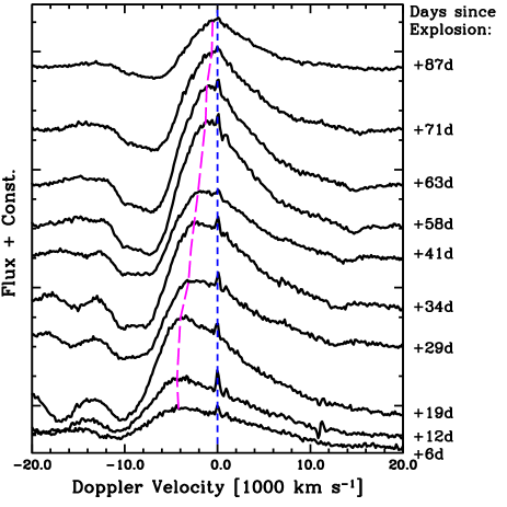
Figure 1: H$\alpha$ spectral sequence of SN 2007X. The rest velocity of the SN position, as measured from the host H ii region narrow H$\alpha$ emission, is indicated by the short dashed blue line (i.e. at zero velocity). The long dashed magenta line shows the evolution of the Doppler velocity of the emission peak.

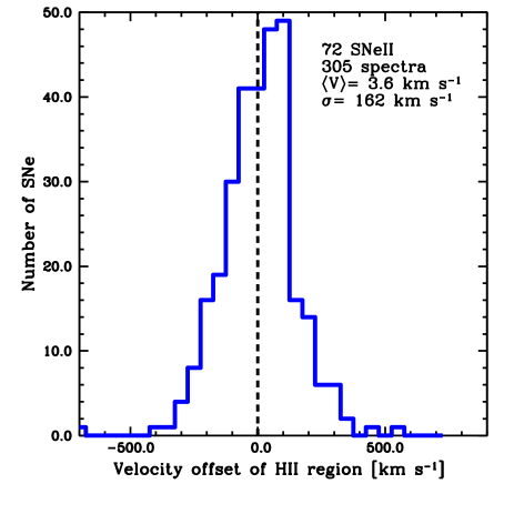
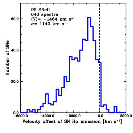
Figure 2: Top: Histogram showing the velocity of the narrow peak emission (associated with a coincident H ii region) detected in each SN spectrum, and given with respect to the host galaxy recession velocity. Bottom: Histogram of the distribution of velocity offsets of H$\alpha$ SN emission for the entire sample of type II SN spectra (corresponding to different post-explosion epochs).

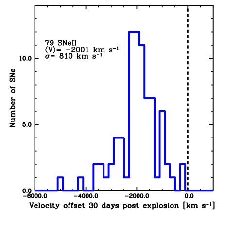
Figure 3: Histogram of the distribution of SN H$\alpha$ emission velocity offsets for observations at 30 d after explosion.

2 Data and analysis methods

The data sample was obtained through various SN follow-up campaigns. These are: 1) the Cerro Tololo SN program (CT, PIs: Phillips & Suntzeff, 1986-2003); 2) the Calán/Tololo SN program (PI: Hamuy 1989-1993); 3) the Optical and Infrared Supernova Survey (SOIRS, PI: Hamuy, 1999-2000); 4) the Carnegie Type II Supernova Program (CATS, PI: Hamuy, 2002-2003); and 5) the Carnegie Supernova Project (CSP, Hamuy et al. 2006, PIs: Phillips & Hamuy, 2004-2009). An initial analysis of the $V$-band light-curve morphologies of this sample has recently been published in Anderson et al. (accepted), and we refer the reader to that paper for in-depth description of SN light-curve parameter measurements. In addition, an initial analysis of the spectral diversity of SNe II, concentrating on H$\alpha$ profiles, was recently published in Gutierrez et al. (accepted). The data taken from the above follow-up programs used in the current analysis amounts to 646 optical wavelength spectra of 95 SNe II. From the above surveys, we excluded events classified as type IIn, type IIb, and SN 1987A-like. Furthermore, we only include in the current analysis SNe which have well-constrained explosion epochs (see below), and more than two spectral observations during the photospheric phase. We note that the follow-up surveys contributing to the current sample were magnitude limited.
Spectra were reduced and extracted in the standard way, and the reader is referred to Folatelli et al. (2013) for a detailed outline of the procedures employed (see also Hamuy et al. 2006). These are analogous to those applied to the CSP SN Ia sample. In summary, 2d spectra were bias subtracted and flat fielded before 1d extraction using the apall task in IRAF. 1d spectra were then wavelength calibrated through observations of arc lamps, and were finally flux calibrated using observations of spectrophotometric standard stars. The typical RMS of individual wavelength solutions less than 0.4 Å, hence this uncertainty brings negligible error into the velocity estimations. The database of spectra were obtained with many different telescopes and instruments. Typically the extracted 1d spectra have wavelength resolutions between 5–8 Å, corresponding to velocity resolutions of 230–370 km s^-1. The S/N ratio of spectra vary, depending on object brightness and distance from the observer. In the majority of cases the S/N of the 1d spectra near to the H$\alpha$ wavelength region of interest is more than 20.
To proceed with measuring the wavelength (and therefore velocity) shift of H$\alpha$ emission peaks, we take host galaxy heliocentric recession velocities from NED, and use these to place the observed spectra on to the rest wavelength of the SNe. In addition, many SNe II show the presence of narrow emission lines in their spectra due to H ii regions at the SN site. When available, these give a more accurate Doppler velocity for the SN environment. Hence, we measure the wavelength of these regions as a) a sanity check of host galaxy recession velocities, and b) to use these in place of host galaxy recession velocities where measurements are possible (this distribution is further discussed below, and is presented in Fig.2).
The emission peak wavelength of the SN H$\alpha$ profile (and the wavelength of the narrow host H ii region) in each spectrum of the sequence for each object is measured. This is done by employing the splot routine in IRAF. Within splot the ‘k’ measurement is used to fit a single Gaussian to the emission part of the P-Cygni profile. The presence of narrow H$\alpha$ from an underlying HII region can complicate the measurement of this peak. Therefore, in cases where strong H$\alpha$ emission dominates over the H$\alpha$ from the SN we do not include measurements from those spectra. Where narrow H$\alpha$ is present but weaker, then this is removed from the spectra by simply tracing a line across the base of its flux. Once the above has been taken into consideration, we fit the emission multiple times, changing the wavelength range used, until a fit is found to be satisfactory ‘by-eye’ (i.e. that the peak of the Gaussian coincides with the peak of the emission). Through this process measurements are obtained using a wavelength window of around $\pm$ 50–100 Å, around the wavelength of the peak emission. Once a peak wavelength is measured it is converted to a SN velocity using the inferred recession velocity, as described above. When the host galaxy recession velocity is employed, this brings a velocity error of $\approx$ 200 km s^-1 (in extreme cases) due to the fact that recession velocities are measured at galaxy centres, while SNe explode at a range of galacto-centric distances, and hence due to galaxy rotational velocities, could have rest velocities offset from those published in the literature (note, this is a very conservative error estimate: see Fig.2). In addition, from our experience measuring peak emission wavelengths, any single spectral measurement has an error of several hundred km s^-1 (due to the difficulty in defining the peak, together with the spectral resolution of each observation). Hence, we assume a conservative error of 500 km s^-1 on all SN velocity measurements.
An example spectral sequence is shown in Fig. 1, where there is clear evidence for a significant blueshift of the SN H$\alpha$ emission peak with respect to the narrow line from a coincident H ii region. In addition, one observes a significant evolution of velocities with time, in particular of the emission-peak offset.
Before continuing to our results, we note that while this work concentrates on the observed wavelength/velocity of the H$\alpha$ emission peak, significant velocity offsets are also found for the emission peaks of other spectral features. At early times one observes very similar strength velocity offsets for the emission peak of H$\beta$. However, after several weeks post explosion, an accurate measurement becomes impossible because of the increased effects of line blanketing, in particular the overlap with neighbouring Fe  ii lines. Hence, one cannot follow the evolution of H$\beta$ emission velocity for more than a few weeks after explosion. Another complication is that some spectral features are absent at early times, and so only appear when line blanketing and line overlap are strong. This is for example a problem with the spectral feature at 4450 Å seen in the earliest spectra of SN 2006bp (Quimby et al., 2007) and SN 1999gi (Leonard et al., 2002a), which indeed models predict to be He  ii 4686 Å but strongly blue shifted due to a very steep density gradient in the photospheric regions at early times (Dessart et al., 2008). H$\alpha$ is by far the strongest line in emission in SN II spectra, and is present at all epochs. This line is thus ideally suited for the study presented here, and we continue using H$\alpha$ as the tracer of velocity-shifted emission features for the remainder of this paper.

3 Results

In Fig. 2 (top panel), the distribution of velocities of narrow H$\alpha$ emission (associated with the coincident H ii region) with respect to host galaxy recession velocities is presented. This distribution contains 305 spectra for 72 SNe II in our sample, and the mean velocity offset is 4 km s^-1: i.e. essentially zero. The standard deviation of this distribution is 162 km s^-1. These values match expectations, since published host galaxy recession velocities will generally be velocities for the centre of each galaxy, whereas SNe will be distributed throughout the galaxy and hence will be found at velocities with a distribution centred on zero and a standard deviation equal to expected rotational velocities of spiral galaxies.
In Fig. 2 (bottom panel), we present the velocity offset distribution of the (broad) SN H$\alpha$ emission peaks for all SNe spectra within our sample. It is immediately apparent that the distribution is heavily offset to significant negative velocities. Indeed, only 4 % of events have positive velocities (red-shifted emission peaks). The mean velocity offset is –1464 km s^-1 with a standard deviation of 1140 km s^-1.
As noted above, when one observes spectral sequences of SNe II, it is quite obvious that the blueshift of lines evolves significantly with time. In Fig. 1, this evolution is shown for SN 2007X. To compare SNe in terms of absolute blue-shifted velocities one needs to measure such a velocity at a consistent epoch. We adopt a post-explosion time of 30 d, where explosion epoch estimates are taken from Anderson et al. (accepted), and interpolate measured velocities to this time. This early epoch is used because it corresponds to times when the diversity of blue-shifted velocities is high (see Fig. 4). It also allows a significant fraction of the SN sample to be included, because numerous SNe in our sample lack spectroscopic data prior to a month after explosion. We note that the typical errors on our explosion epochs are $\pm$ 6 days (taken from Anderson et al. accepted). The epochs used to interpolate velocities to 30 d  are generally within $\sim$ 5–15 days either side of this epoch. The distribution of velocity offsets at 30 d post explosion is presented in Fig. 3. The startling feature of this plot is that SNe have exclusive blue-shifted velocities at this epoch. Indeed, the mean of the distribution is –2001 km s^-1 with a standard deviation of 810 km s^-1. The other interesting feature of the figure is the high velocity tail out to $\sim$ 4000 km s^-1. The overriding conclusion from the distributions presented above is that significant blue-shifted emission velocities on the order of several thousand km s^-1 are a ubiquitous feature in SN II spectra.
After presenting the distribution of the velocity offsets of H$\alpha$ emission peaks at a representative post-explosion epoch, we now turn our attention to their evolution with time. In Fig. 4, this evolution is displayed for all 95 SNe in our sample. While there is significant scatter at all epochs, a number of interesting features are observed. Firstly, the highest velocities are exclusively seen at early times. Very few SNe show blue-shifted emission peaks higher than 2000 km s^-1 after 50 d post explosion, while at early times there is a significant number of SNe with velocities in excess of 3500 km s^-1. Secondly, the dispersion in velocity appears to decrease significantly with time.
In summary, significant blue-shifted velocities of several thousand km s^-1 are a very common feature of type II SN spectra. These velocities evolve in time quite uniformly between SNe, eventually nearing zero as they progress to the end of the photospheric phase. In the following Section we discuss model spectra known to match the basic properties of SNe II-P (Dessart et al., 2013), as well as the theoretical framework for understanding the origin of emission-peak blueshifts.

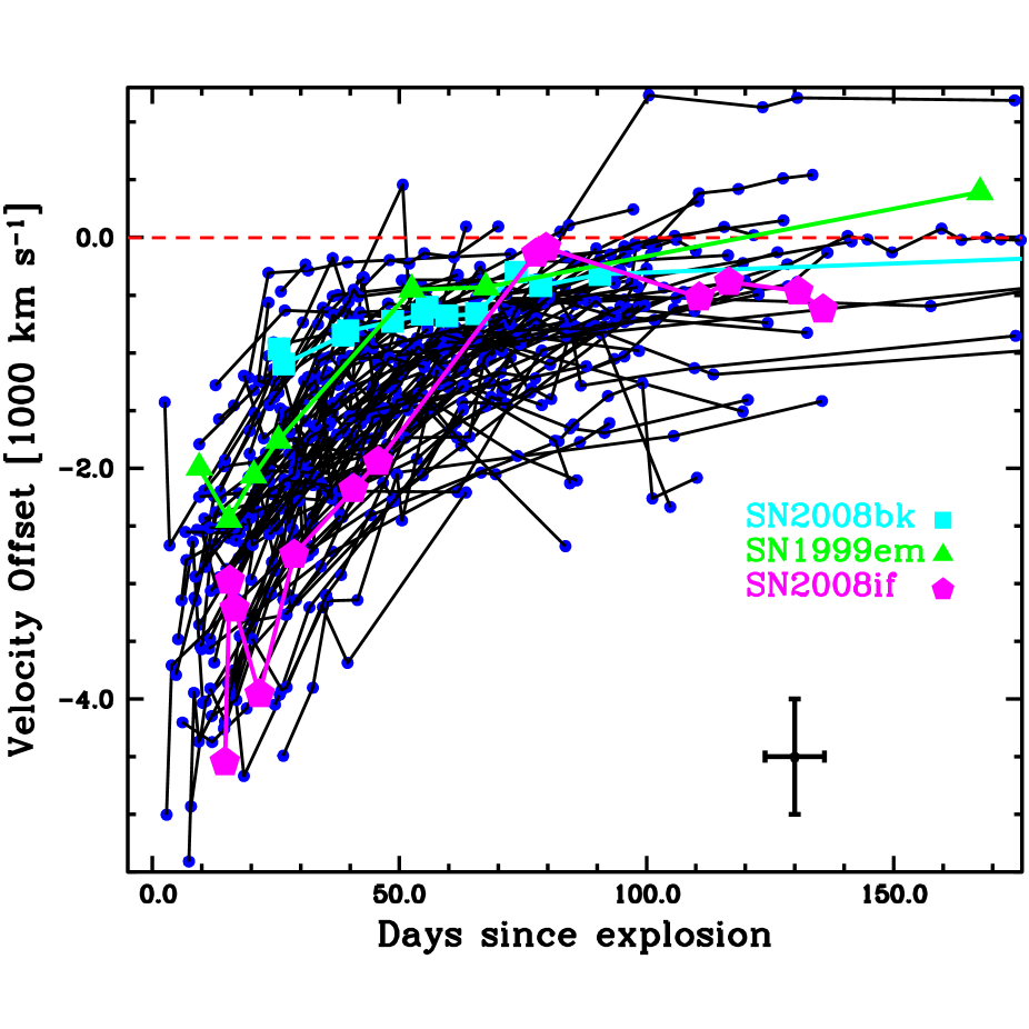
Figure 4: Evolution in time of the velocity offset of SN H$\alpha$ emission peaks for the 95 SNe II in the current sample. Three events are shown: a sub-luminous event, SN 2008bk; a prototype type II-P, SN 1999em; and a faster declining event, SN 2008if. A standard error bar for all measurements is given in black, where the origin of the velocity error is outlined in § 2, and the time error is based on average errors of estimated explosion epochs (see Anderson et al. accepted, for a detailed description of that process).

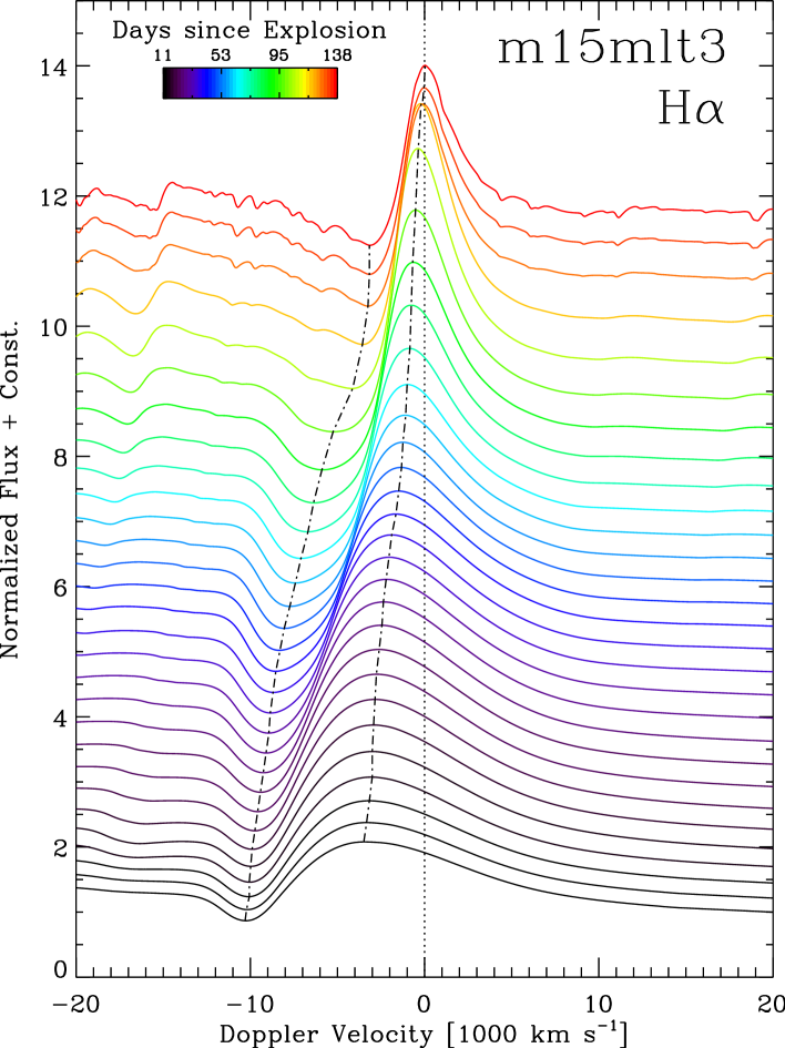
Figure 5: Evolution of the H$\alpha$ spectral region from 11 d (bottom curve) until 138 d (top curve) after explosion in the SN II-P model m15mlt3 (Dessart et al., 2013). The abscissa is the Doppler velocity with respect to H$\alpha$. Individual times are color coded, and the time difference between consecutive models is 10%̇ of the current time. The two broken lines track the location of maximum absorption and peak emission in H$\alpha$. The peak blueshift, strong at early times, decreases as the spectrum formation region recedes, and eventually becomes zero at the end of the plateau phase (in this model at $\sim$ 140 d).

4 Insights from radiative-transfer simulations

4.1 Previous studies with cmfgen

As documented in the previous Section, the offset of P-Cygni profile emission to the blue is a ubiquitous feature of all SNe II observed during the photospheric phase. In this Section, we investigate whether this generic property is also present in spectra produced by radiative-transfer simulations of SNe II.
Spectrum formation for SNe II has been studied previously with cmfgen. In Dessart & Hillier (2005a, b), steady-state non-LTE simulations were used to discuss the physics of P-Cygni profile formation in early time spectra of SNe 1987A and 1999em. The peak blueshift is reproduced for both events prior to the recombination phase, and a detailed discussion of the origin of this property is given in § 5 of Dessart & Hillier (2005a). Later, in Dessart & Hillier (2008), the discussion is extended to more advanced photospheric-phase epochs, when the photospheric layers recombine, using a time-dependent solver for the non-LTE rate equations. This study focused primarily on the importance of time-dependent ionization, and in particular its role for producing a strong H$\alpha$ line at the recombination epoch — little emphasis was put on the peak blueshift.
In Dessart et al. (2013), the radiative transfer in cmfgen was improved by combining non-LTE and time dependence (for the non-LTE rate equations and the moments of the radiative-transfer equation). In addition, the computation is then performed on physically-consistent (although piston-driven) hydrodynamical explosions (see Hillier & Dessart 2012 for details and Dessart & Hillier 2010 for an application to SN 1987A). Moreover, these simulations cover a range of progenitor evolution and explosion properties for a 15 ${\rm\ M}_{\odot}$ main-sequence star model and therefore allow one to inspect a number of dependencies on SN II-P radiation properties.
In the present paper, we inspect the simulations of Dessart et al. (2013), with a special focus on the evolution of line profile morphology from early photospheric epochs to the onset of the nebular phase. We focus on a representative sample of models, namely s15N, m15r1, m15r2, m15os m15mlt1, m15mlt3, m15, m15e3p0, m15e0p6, and m15Mdot (see Dessart et al. 2013 for details; these models cover a range of properties for the same main-sequence star mass but different initial rotation rate, mixing-length parameter, core overshooting prescription, or explosion energy). We also include model m15mlt1x3, which is evolved the same way as m15 but with a mixing-length-parameter of 1.5 and a mass loss enhanced by a factor of three compared to the standard red-supergiant (RSG) mass loss rates provided by the ‘DUTCH’ recipe in mesa. This produces a low envelope-mass RSG at the time of explosion, which, when exploded to yield a 1.2 B ejecta kinetic energy, yields a Type II-Linear light-curve morphology (see Hillier et al., in prep.).

4.2 Results for SN II-P simulations

The first important result is that the peak-emission blueshift, observed in spectra of SNe II (see, e.g., Fig. 1) is also predicted by simulations at all times prior to the onset of the nebular phase. Figure 5 shows the evolution of the H$\alpha$ region from 11 d until 138 d after explosion in model m15mlt3. This model matches well the spectral and light curve evolution of SN 1999em, except for a prolonged plateau phase of $\mathrel{\hbox{\hbox to0.0pt{\hbox{\lower 4.0pt\hbox{$\sim$}}\hss}\hbox{$<$}}}$150 d, which stems for the underestimated RSG mass loss in the mesa model (see Dessart et al. 2013 for details). The evolution of the velocity offset of peak emission agrees qualitatively and quantitatively with the observations. Importantly, all the simulations presented in Dessart et al. (2013) show the same behaviour, in agreement with observations (Fig. 6). Typical peak blueshifts are on the order of $-$3200 km s^-1 at 10 d after explosion and steadily decrease in strength to eventually reach zero at the end of the plateau, as observed.

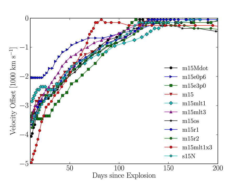
Figure 6: Evolution of the velocity offset of H$\alpha$ peak emission with respect to rest wavelength for the large set of models presented in Dessart et al. (2013). All models follow the same trajectory, except for models m15e3p0/m15e0p6 (3 and 0.6 B, respectively), which have a larger/lower ejecta energy than other models (i.e., 1.2 B), and for model m15mlt1x3, in which the RSG mass loss was artificially increased by a factor of 3. [See text for discussion].

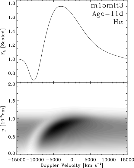
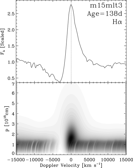
Figure 7: Distribution of the quantity $p\times I(p)$, as seen by a distant observer at rest, versus Doppler velocity $v$ and impact parameter $p$ (lower panels). When integrated over $p$, this gives the flux at $v$ (upper panels). Here, we show a SN II-P model at 11 d (left) and 138 d (right) after explosion. The grayscale maps thus reveal the origin of the emergent radiation in different profile regions (Doppler velocity) along rays with different $p$. The main reason for the blueshift is the confinement of emission within the column of material falling onto the ‘photo disk’. This disk is limited on the plane of the sky by an impact parameter $p$ on the order of $R_{\rm phot}$. Because of obscuration effects, and the lack of line emission at large impact parameters, the emission comes primarily from regions that are blue shifted, and this naturally leads to peak-emission blueshift. At late times (right panel), obscuration effects are still present, but there is now significant emission at large impact parameters, which occurs symmetrically from approaching and receding regions. In fact, photon emission is more extended at all wavelengths, stemming both the former He core and the H-rich envelope.

5 Discussion

In previous sections it has been shown that significant blue-shifted velocities of H$\alpha$ emission peaks are a common feature of both observations and models of SNe II. Here we first discuss the physical origin of these features and their diversity, before presenting two correlations of this property with other SNe II transient measurements.

5.1 The physical origin of blue-shifted emission peaks

In contrast to Chugai (1988), the origin of peak-emission blueshift seems to stem fundamentally from the steep density profile that characterizes SN ejecta layers, which were originally part of the H-rich envelope. In our simulations, this density distribution is well represented above $\sim$ 2000 km s^-1 (which is roughly where the outer edge of the former He-core lies in 1.2 B explosions of 15 ${\rm\ M}_{\odot}$ RSG stars; Dessart et al. 2010) by a power law $\rho(v)\propto 1/v^{n}$, with exponent $n$ on the order of 8. As a consequence, line emission tends to be confined in space, and subject to strong occultation effects for a distant observer. Instead of coming predominantly from the regions with large impact parameter $p$ relative to the photospheric radius $R_{\rm phot}$ the bulk of the emission arises from rays with $p<R_{\rm phot}$, i.e. impacting the photo-disk limited by $p=R_{\rm phot}$. As explained in Dessart & Hillier (2005b), the line source function tends to exceed the continuum source function at the continuum photosphere, naturally leading to line emission above the continuum flux level. Because electron-scattering dominates the opacity, line photons have a relatively low destruction probability and we can therefore see line emission from layers deeper than the continuum photosphere.
Fig. 7 illustrates these effects for model m15mlt3 at 11 d (left panel). As time progresses, the situation evolves significantly for several reasons. The spectrum formation recedes to deeper layers in the ejecta, where the density profile is flatter, favouring extended emission above the continuum photosphere. The velocities are also lower, so any velocity offset becomes less conspicuous. Moreover, time-dependent ionization exacerbates this effect by making the line optical depth more slowly varying with radius/velocity (Dessart & Hillier, 2008), also favouring extended line emission. Interestingly, it is in part the increase in the extension of the spectrum formation region that favours the rise of polarization at the end of the plateau phase in SNe II-P (Dessart & Hillier, 2011).
Departures from the mean trajectory of the peak location in velocity space of emission peaks are visible for three models in Fig. 6. First, the two models with a lower/higher kinetic energies (models m15e0p6 and m15e3p0) show smaller/larger offsets, simply reflecting the contrast in ejecta velocity (same envelope mass $M$, but different kinetic energy $E$). In these, the peak blueshifts at 10 d after explosion are $-$2000 km s^-1 and $-$3500 km s^-1 respectively. Second, model m15mlt1x3, which has a higher ejecta kinetic energy to ejecta mass (same $E$ of 1.2 B as the models of Dessart et al. 2013, but much lower H-envelope mass), shows a markedly different trajectory for the peak-emission offset. Because the expansion rate is much larger, the offset is large initially, but the reduced envelope mass makes the transition to nebular phase earlier, and at such times the offset is always found to be zero in our models. Thus, the rate of change of this offset is much larger in model m15mlt1x3. This is an interesting property which is also seen in observations. Indeed, SNe with a higher $s_{2}$ parameter (i.e., $V$-band light curves with steeper decline rates) also have larger initial velocity offsets (see Fig. 8).

5.2 Correlation with other SN properties

While a full investigation into how observations of blue-shifted emission are related to other SN properties is beyond the scope of this paper, in this Section we outline a couple of interesting correlations that have been found, and suggest how these may be used to further understand the nature of SNe II. In Fig. 8 the decline rate during the ‘plateau’, $s_{2}$ (which is a proxy for the degree to which a type II SN could be classified as ‘Linear’: see Anderson et al. accepted), is plotted against the SN emission peak velocity offset measured at 30 d post explosion (only SNe which have both $s_{1}$ –the initial decline from maximum– and $s_{2}$ defined are included, see Anderson et al. accepted for justification of this). A correlation is found in that faster declining SNe show higher velocity offsets at the same epoch as compared to smaller $s_{2}$ SNe. To test the significance of this correlation we employ a Monte Carlo application of the Pearson’s test for correlations (following the procedure outline in Anderson et al. accepted). A Pearson’s r-value of $-0.75\pm 0.10$ is calculated, which, for $N=24$ equates to a lower limit significance $P=6\times 10^{-4}$ (i.e. the probability of finding a correlation by chance). It is interesting that in the synthetic measurements displayed in Fig. 6, the highest velocity offsets at around 30 d post explosion are for the model (m15mlt1x3), which has a more ‘Linear’ light-curve morphology (i.e. a high $s_{2}$). As discussed in Section 4.2, model m15mlt1x3 is characterized by the same ejecta kinetic energy of 1.2 B as other models from Dessart et al. (2013), but its ejecta mass is smaller. This translates to a higher expansion rate and a shorter photospheric phase duration, hence a larger H$\alpha$ peak offset early on together with its more rapid decrease to zero.
In Fig. 9, SNe maximum $V$-band magnitudes are correlated against SN emission peak velocity offsets measured at 30 d post explosion. A strong correlation is found in terms of brighter SNe showing higher velocity offsets (confirmed by a Monte Carlo application of the Pearson’s test: $N=51$, $r=0.75\pm 0.07$ $P<2\times 10^{-8}$). The strength of this correlation is quite remarkable given the uncertainties in measurements of $M_{\text{max}}$ (problems in defining this epoch, issues with host galaxy extinction corrections), the explosion epoch estimations (see discussion in Anderson et al. accepted), together with those of the velocity offsets. Here again, our more ‘Linear’ type II SN model m15mlt1x3 offers a promising explanation (together with the possibility of diversity being related to explosion energy differences). Indeed, it exhibits a much higher luminosity than other SNe II-P models in Dessart et al. (2013), although it has the same explosion energy. The difference here is that this energy is coupled to a smaller progenitor envelope mass, leading to a higher energy per unit mass, a higher luminosity early on with a larger expansion rate. Because the ejecta mass is lower, the photospheric phase is shorter and so the luminosity decreases earlier and faster until reaching the nebular phase. In that context, this observation would support the notion that the diversity of SNe II-P, in particular the smooth connection to type II SNe with more ‘Linear’ light curves (Anderson et al., accepted, although see Arcavi et al. 2012 for claims of a distinct separation between SNe II-P and SNe II-L), stems from a diversity in progenitor envelope mass. This hypothesis is discussed at length in Anderson et al. (accepted) with respect to the diversity seen in the $V$-band light-curves of 116 SNe II. Of course, this does not preclude the additional diversity stemming from varying explosion energies.
In the context of the current analysis, the diversity of the observed (and predicted) strength of blue-shifted emission velocities can then be understood in terms of changes in the pre-SN envelope mass and/or differences in explosion energy. As one decreases the envelope mass (or increases the explosion energy), ejecta velocities increase due to the higher energy per unit mass. The strength of the blue-shifted emission velocity is then directly linked to the ejecta velocity. This energy increase also increases the early luminosity (hence a higher $M_{\text{max}}$, as observed in Fig. 9), while the faster expansion leads to faster declining light-curves, and hence the correlation observed with $s_{2}$ in Fig. 8.
Finally, we note that the correlation presented in Fig. 9 implies that measurements of the blueshift of H$\alpha$ emission profiles could be used to predict SN absolute magnitudes. In this sense, such a correlation could be used as another SN II distance indicator method (to complement other such methods: e.g. Hamuy & Pinto 2002). The RMS scatter of the trend found in Fig. 9 is $\sim$0.68 mag, however one may hope to further improve this with a more detailed analysis (e.g. better constraints on host extinction, the use of colour information). As noted in § 2, the follow-up surveys which contributed to the current sample were magnitude limited in nature. Hence, if the correlation presented in Fig. 9 holds, then surveys such as the CSP will preferentially follow SNe with larger blue-shifted velocity offsets.

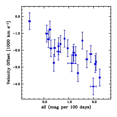
Figure 8: $s_{2}$ (the decline rate during the ‘plateau’) plotted against the velocity offset of SNe H$\alpha$ emission peaks at 30 d post explosion.

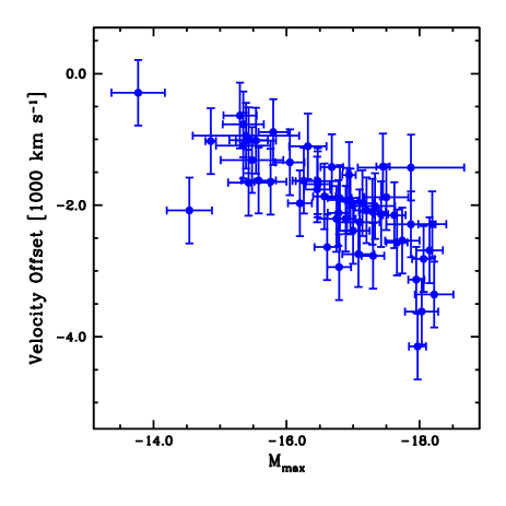
Figure 9: $M_{\text{max}}$ (absolute magnitude at maximum light in the $V$-band) plotted against the velocity offset of SNe H$\alpha$ emission peaks at 30 d post explosion.

6 Conclusions

We have presented an observational analysis which shows that blue-shifted emission peaks are seen in all spectral sequences of SNe II. These blue-shifted velocity offsets are observed to be larger at early times and evolve to being consistent with zero once SNe enter their nebular phase. Hence, peak-emission blueshifts are generic properties of observed SN II spectra. In addition, we demonstrate that emission-peak blueshifts are also a generic feature of photospheric-phase SN II spectra computed with the non-LTE time-dependent radiative-transfer code cmfgen and based on physical models of the progenitor star and explosion. In fact, such blueshifts occur not just in SNe II, but also in SNe Ia (Blondin et al., 2006), although line overlap complicates a clear identification of such offsets. In SNe II, the velocity offset is best seen in H$\alpha$, because the line is strong, but also because one can track the velocity offset from being large early on to becoming negligible when the SN turns nebular.
In addition, we have shown that the diversity of blue-shifted velocities found within a large sample of SNe II, can also be linked to SN II light-curve diversity. SNe showing larger blueshifts are also found to be brighter objects, and have faster declining light-curves. We speculate that this diversity and the trends observed between different parameters, can be most easily understood in terms of differences in proegnitor envelope masses retained before the epoch of explosion.
Until now, measurements, analysis and discussion of these properties for SNe of any kind have been scarce, despite the fact that their presence is obvious and systematic. As our analysis and discussion show, these features and their evolution systematically change between SNe, and offer additional leverage to identify the origin of the diversity in SN II observations, progenitors, and explosion.

References

- Arcavi et al. (2012) Arcavi I., et al., 2012, ApJ Let., 756, L30
- Blondin et al. (2006) Blondin S., et al., 2006, AJ, 131, 1648
- Bose et al. (2013) Bose S., et al., 2013, MNRAS, 433, 1871
- Cappellaro et al. (1995) Cappellaro E., Danziger I. J., della Valle M., Gouiffes C., Turatto M., 1995, A&A, 293, 723
- Castor (1970) Castor J. I., 1970, MNRAS, 149, 111
- Chevalier (1976) Chevalier R. A., 1976, ApJ, 207, 872
- Chugai (1988) Chugai N. N., 1988, Soviet Astronomy Letters, 14, 334
- Dessart et al. (2008) Dessart L., et al., 2008, ApJ, 675, 644
- Dessart & Hillier (2005a) Dessart L., Hillier D. J., 2005a, A&A, 439, 671
- Dessart & Hillier (2005b) Dessart L., Hillier D. J., 2005b, A&A, 437, 667
- Dessart & Hillier (2008) Dessart L., Hillier D. J., 2008, MNRAS, 383, 57
- Dessart & Hillier (2010) Dessart L., Hillier D. J., 2010, MNRAS, 405, 2141
- Dessart & Hillier (2011) Dessart L., Hillier D. J., 2011, MNRAS, 415, 3497
- Dessart et al. (2013) Dessart L., Hillier D. J., Waldman R., Livne E., 2013, MNRAS, 433, 1745
- Dessart et al. (2010) Dessart L., Livne E., Waldman R., 2010, MNRAS, 408, 827
- Elmhamdi et al. (2003) Elmhamdi A., Danziger I. J., Chugai N., Pastorello A., Turatto M., Cappellaro E., Altavilla G., Benetti S., Patat F., Salvo M., 2003, MNRAS, 338, 939
- Filippenko (1997) Filippenko A. V., 1997, ARA&A, 35, 309
- Folatelli et al. (2013) Folatelli G., et al., 2013, ApJ, 773, 53
- Fraser et al. (2011) Fraser M., et al., 2011, MNRAS, 417, 1417
- Hamuy et al. (2001) Hamuy M., et al., 2001, ApJ, 558, 615
- Hamuy et al. (2006) Hamuy M., et al., 2006, PASP, 118, 2
- Hamuy & Pinto (2002) Hamuy M., Pinto P. A., 2002, ApJ Let., 566, L63
- Hillier & Dessart (2012) Hillier D. J., Dessart L., 2012, MNRAS, 424, 252
- Leonard et al. (2002a) Leonard D. C., et al., 2002a, AJ, 124, 2490
- Leonard et al. (2002b) Leonard D. C., et al., 2002b, PASP, 114, 35
- Menzies et al. (1987) Menzies J. W., et al., 1987, MNRAS, 227, 39P
- Minkowski (1941) Minkowski R., 1941, PASP, 53, 224
- Quimby et al. (2007) Quimby R. M., Wheeler J. C., Höflich P., Akerlof C. W., Brown P. J., Rykoff E. S., 2007, ApJ, 666, 1093
- Sobolev (1960) Sobolev V. V., 1960, Moving envelopes of stars
- Turatto et al. (1993) Turatto M., Cappellaro E., Benetti S., Danziger I. J., 1993, MNRAS, 265, 471