BCS instabilities of electron stars to holographic superconductors

Abstract

We study fermion pairing and condensation towards an ordered state in strongly coupled quantum critical systems with a holographic AdS/CFT dual. On the gravity side this is modeled by a system of charged fermion interacting through a BCS coupling. At finite density such a system has a BCS instability. We combine the relativistic version of mean-field BCS with the semi-classical fluid approximation for the many-body state of fermions. The resulting groundstate is the AdS equivalent of a charged neutron star with a superconducting core. The spectral function of the fermions confirms that the ground state is ordered through the condensation of the pair operator. A natural variant of the BCS star is shown to exist where the gap field couples Stueckelberg-like to the AdS Maxwell field. This enhances the tendency of the system to superconduct.

I Introduction

Gauge/gravity duality has given us a number of qualitatively new insights into the physics of quantum critical systems. Notably these include a controlled theoretical framework for non-Fermi liquids Liu:2009dm ; Cubrovic:2009ye ; Faulkner:2009wj ; Faulkner:2010tq as well as an onset towards superconductivity that is distinct from BCS and goes beyond Landau-Ginzburg Hartnoll:2008vx ; Hartnoll:2008kx ; She:2011cm . (See e.g. Iqbal:2011ae for a review.) The obvious candidates where both phenomena are seen experimentally are the unconventional high $T_{c}$ superconductors, and one has reason to hope that gauge-string duality may be able to explain some its open mysteries.

The clearest puzzle that must be solved to do so, is that one needs a single holographic model that describes both the non-Fermi-liquid metals and high $T_{c}$ superconductors simultaneously. Intuitively this sounds obvious, as the sole charge carriers are the fermionic electrons; it is their behavior which becomes non-Fermi liquid-like, while they are simultaneously responsible for the onset of superconductivity through $d$-wave pairing. This intuition should not be taken as holy, however. At strong coupling by definition the underlying electron picture fails, and one should consider a different weakly coupled set of elementary excitations. In essence this is what gauge-gravity duality can do very well. For example, in the specific top-down holographic example of $N=2$ SYM with flavor, where one knows the explicit Lagrangian of the dual CFT, one can construct a holographic superconductor where the order parameter is identified with a strongly coupled Cooper pair of fermionic ``mesino'' fields erdmenger .

In a bottom-up phenomenological direction, early studies that combine pairing with ordering are Faulkner:2009am and Hartman:2010fk which studied the formation of a gap in fermion spectral functions in a holographic superconductor groundstate and the tendency for holographic non-Fermi liquids to pair and condense. In this paper we make a simple further step in the direction. The aim is to phenomenologically describe a holographic model where fermion pairing is fully responsible for the superconducting groundstate. We start from a bulk system with only fermionic matter fields coupled to gravity and Maxwell field. We include an attractive four point interaction for the bulk fermions and, approximating the many-body fermions in the fluid limit, we solve this self-gravitating charged interacting fermi fluid in an asymptotically AdS background at zero temperature. Thus in fact the bulk is a fluid of local BCS vacuum states. More complicated versions of this system are known in the astrophysics community that studies neutron stars with superconducting cores. We show evidence that the holographic dual state to the core-superconducting electron star is also the pairing induced superconducting state.

In this construction, the advantages are that the fluid limit makes it practical to extract the macroscopic information of the dual state. Moreover all the charge is carried by fermions so that the origin of the boundary charged degrees of freedom is manifest. However, this construction has the well-known drawback of the fluid limit that the fermionic fields are not visible at the boundary. We can nevertheless still discern boundary effects using the charge distribution within the star as we will show later. In a companion article inprogress2 one of us will discuss the same system treating the fermions quantum mechanically Sachdev:2011ze ; Allais:2012ye ; Allais:2013lha . To place our work in the context of the previous approaches Faulkner:2009am ; Hartman:2010fk , we also discuss a more generalized model which includes an independent charged scalar field with dynamics. In the star limit, parameters and fields in this system will get rescaled and not all the terms in the Lagrangian can be kept at the same time. In particular the kinetic term always vanishes except in the neutral case. In addition to the limit where one goes back to the bulk BCS system, there exists a more subtle limit, which we also discuss.

Let us conclude by emphasizing that we will be studying the zero-temperature quantum phase transition between the holographic dual of the (Russian doll multi-band) Fermi liquid (the electron star) and the pair-ordered BCS groundstate (a star with a BCS core) as a function of the BCS coupling. In Sec. II we will first construct our BCS star and show that it is more stable than the electron star solution at zero temperature. In Sec. III we show evidence that the bulk BCS star system will correspond to a superconducting state at the boundary. Then we introduce a more generalized model in Sec. IV and discuss one scaling limit that is different from the BCS star one. We conclude in Sec. V.

II A BCS star

BCS theory bcs was proposed by Bardeen, Cooper and Schrieffer in 1957 as the explanation of low temperature superconductivity through the pairing of fermions into a bosonic state which subsequently condenses at low temperatures. Starting with a Fermi liquid, BCS theory introduces an attractive interaction between fermions at the Fermi surface. This interaction induces an instability to the formation of Cooper pairs of fermions. Microscopically this effective attractive interaction results from exchange of phonons and is constrained in a region $(-\omega_{D},\omega_{D})$ near the Fermi surface $E_{F}$ or equivalently the chemical potential $\mu$. Here $\omega_{D}$ is the Debye frequency, a characteristic scale of phonon excitations. The simplest effective (non-relativistic) Hamiltonian describing the physics of a thin shell of states of width $2\omega_{D}$ centered around the Fermi surface can be written as

$$H=\sum_{{\bf k}\sigma}\epsilon_{{\bf k}}c^{\dagger}_{{\bf k}\sigma}c_{{\bf k}\sigma}-\frac{\lambda}{V}\sum_{{\bf k},{\bf k}^{\prime},{\bf q}}c^{\dagger}_{{\bf k}+{\bf q}\uparrow}c^{\dagger}_{-{\bf k}\downarrow}c_{-{\bf k}^{\prime}+{\bf q}\downarrow}c_{{\bf k}^{\prime}\uparrow},$$ (1)

where $\lambda$ is a positive constant, ${\bf k},{\bf k}^{\prime},{\bf q}$ denote the momentum, $\sigma=\left\{\uparrow,\downarrow\right\}$ denotes the spin and $\epsilon_{\bf k}$ is the kinetic energy of free fermions.

Here we couple the relativistic version of the BCS system to gravity. The bulk gravity system we consider is the Einstein-Maxwell-BCS system:

$$\mathcal{L} = \frac{1}{2\kappa^{2}}\bigg{(}R+\frac{6}{L^{2}}\bigg{)}-\frac{1}{4e^{2}}F_{\mu\nu}F^{\mu\nu}+\mathcal{L}_{\text{BCS}},$$ (2)

where $\kappa$ is the gravitational coupling constant, $e$ is the Maxwell coupling constant. $\mathcal{L}_{\text{BCS}}$ is the relativistic Lagrangian of the BCS system thesis ; Hartman:2010fk , which is a direct generalization of (1)

$$\mathcal{L}_{\text{BCS}}=-i\bar{\Psi}(\Gamma^{\mu}\mathcal{D}_{\mu}-m_{f})\Psi+\frac{\lambda}{2}(\bar{\Psi}_{c}\Gamma^{5}\Psi)^{\dagger}(\bar{\Psi}_{c}\Gamma^{5}\Psi)$$ (3)

where

$$\bar{\Psi}=\Psi^{\dagger}\Gamma^{\underline{t}},~{}~{}~{}\mathcal{D}_{\mu}=\partial_{\mu}+\frac{1}{4}\omega_{ab\mu}\Gamma^{ab}-iqA_{\mu}.$$ (4)

Here $\lambda$ is a positive coupling constant of mass dimension $[\lambda]=-2$ and $\Psi_{c}=C\bar{\Psi}^{T}$ and the covariant derivative includes the gauge- and spin-connection. We perform a Hubbard-Stratanovich transformation as in the non-relativistic case

$$\Delta=\lambda\bar{\Psi}_{c}\Gamma^{5}\Psi,$$ (5)

to obtain

$$\mathcal{L}_{\text{BCS}}=-i\bar{\Psi}(\Gamma^{\mu}\mathcal{D}_{\mu}-m_{f})\Psi+\frac{1}{2}\Delta^{\dagger}\bar{\Psi}_{c}\Gamma^{5}\Psi-\frac{1}{2}\Delta\bar{\Psi}\Gamma^{5}\Psi_{c}-\frac{1}{2\lambda}|\Delta|^{2}.$$ (6)

The auxiliary field $\Delta$, also known as the BCS ``gap'', can be seen as the order parameter for the BCS condensation. The connection of this system with a kinetic term for a dynamical scalar $\Delta$ will be discussed in Sec. IV.

The equations of motion for this system are

$$R_{\mu\nu}-\frac{1}{2}g_{\mu\nu}R-\frac{3}{L^{2}}g_{\mu\nu} = \kappa^{2}\big{[}T_{\mu\nu}^{~{}\text{gauge}}+T_{\mu\nu}^{~{}\text{BCS}}\big{]};$$

$${\nabla_{\mu}}F^{\mu}_{~{}~{}\nu} = -e^{2}J_{\nu}^{~{}\text{BCS}},$$ (7)

$$i(\Gamma^{\mu}\mathcal{D}_{\mu}-m)\Psi+\Delta\Gamma^{5}\Psi_{c} = 0,$$

where

$$T_{\mu\nu}^{~{}\text{gauge}} = \frac{1}{e^{2}}\big{(}F_{\mu\rho}F_{\nu}^{~{}\rho}-\frac{1}{4}F^{2}g_{\mu\nu}\big{)},$$

$$T_{\mu\nu}^{~{}\text{BCS}} = \frac{1}{2}\langle i\bar{\Psi}\Gamma_{(\mu}\mathcal{D}_{\nu)}\Psi-i\bar{\Psi}\overleftarrow{\mathcal{D}}_{(\mu}\Gamma_{\nu)}\Psi\rangle+g_{\mu\nu}\langle\mathcal{L}_{\text{BCS}}\rangle,$$ (8)

$$J_{\mu}^{~{}\text{BCS}} = -q\langle\bar{\Psi}\Gamma_{\mu}\Psi\rangle.$$

As in Liu:2013yaa , we rescale $qA_{\mu}\to A_{\mu}$ to fix $q=1.$

II.1 BCS fluid in the bulk

As in Hartnoll:2009ns ; deBoer:2009wk ; Arsiwalla:2010bt ; Hartnoll:2010gu , we solve this system in the classical limit $\kappa\to 0$, where we approximate the many-body-fermi system by an effective fluid. This is consistent in the adiabatic limit, where the variation of the electrostatic potential (or local chemical potential) and the gap are small: $\partial_{r}\mu_{l}\ll\mu_{l}^{2}$ and $\partial_{r}\Delta\ll\Delta^{2}$. This adiabatic limit allows a construction of the expectation values in (8) as if the system is in flat spacetime. We compute the expectation values at a fixed local chemical potential $\mu_{l}$ and gap $\Delta$ and then promote these to slowly varying quantities governed by $A_{t}(r)$ and $\Delta(r)$ respectively. Here $r$ is the radial direction of AdS, encoding the effective energy scale of the dual field theory.

To do so remark that the BCS interaction term only exists in an interval $(-\omega_{D},\omega_{D})$ near the Fermi surface, so we can divide the fermion excitations into two parts, the first part with energy from $m_{f}$ to $\mu_{l}-\omega_{D}$ and the second part from $\mu_{l}-\omega_{D}$ to $\mu_{l}+\omega_{D}$. This is illustrated in Fig. 1.

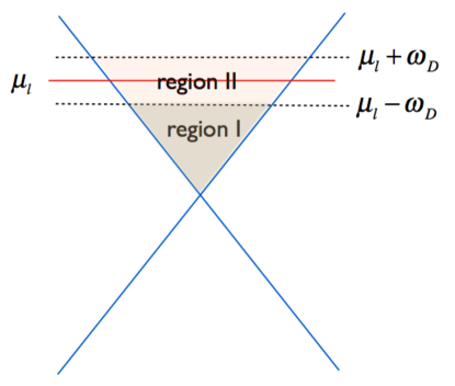
Figure 1: An illustration of the BCS vacuum state. In region I the fermions are still free Fermi gas. In region II, the BCS interaction allows Cooper pairs start to form and one has a BCS state.

In the first region, the bulk fermion system is still that of free fermions (adiabatically coupled to gravity and electromagnetism) which obey the Pauli exclusion principle, so it is straightforward to write out the contribution of fermions in this region to the energy momentum tensor and the current. They are the regular values for many-body fermions in the Thomas-Fermi approximation:

$$T_{\mu\nu}^{\text{FL}_{\text{I}}}=(\rho_{\text{I}}^{\text{FL}}+p_{\text{I}}^{\text{FL}})u_{\mu}u_{\nu}+p_{\text{I}}^{\text{FL}}g_{\mu\nu},$$ (9)

and

$$J^{\mu}_{\text{FL}_{\text{I}}}=n_{\text{I}}^{\text{FL}}u^{\mu},$$ (10)

where

$$\rho_{\text{I}}^{\text{FL}} = \int_{{\bf k}^{2}<\mu_{l}-\omega_{D}}d^{3}{\bf k}\langle{\bf k}|T_{00}|{\bf k}\rangle=\frac{1}{\pi^{2}}\int_{m_{f}}^{\mu_{l}-\omega_{D}}d\omega\omega^{2}\sqrt{\omega^{2}-m_{f}^{2}},$$ (11)

$$p_{\text{I}}^{\text{FL}} = \int_{{\bf k}^{2}<\mu_{l}-\omega_{D}}d^{3}{\bf k}\langle{\bf k}|T_{11}|{\bf k}\rangle=\frac{1}{3\pi^{2}}\int_{m_{f}}^{\mu_{l}-\omega_{D}}d\omega\sqrt{\omega^{2}-m_{f}^{2}}^{3},$$ (12)

$$n_{\text{I}}^{\text{FL}} = \int_{{\bf k}^{2}<\mu_{l}-\omega_{D}}d^{3}{\bf k}=\frac{1}{\pi^{2}}\int_{m_{f}}^{\mu_{l}-\omega_{D}}d\omega\omega\sqrt{\omega^{2}-m_{f}^{2}},$$ (13)

with $n_{\text{I}}^{\text{FL}}$ denotes the number density of free fermions in region I.

In the second region (region II in Fig. 1), due to the interactions with $\Delta$, fermions do not obey the zero temperature Fermi-Dirac distribution anymore. We can first perform a Bogoliubov transformation to make the interacting system tractable. In this interacting region, quasi particles of fermion excitations with opposite momentum and spin near the Fermi surface are coupled together, which introduces off-diagonal elements in the Hamiltonian thesis as

$$H-\mu_{l}N=\sum_{\bf k}\Psi^{\dagger}_{\bf k}\begin{pmatrix}\xi_{\bf k}&-\Delta\\ -\bar{\Delta}&-\xi_{\bf k}\end{pmatrix}\Psi_{\bf k}+\sum_{\bf k}\xi_{\bf k}+V\frac{\Delta^{2}}{2\lambda}$$ (14)

where $\Psi_{\bf k}$ is the Nambu spinor $\Psi_{\bf k}=\begin{pmatrix}c_{{\bf k}\uparrow}\\ c^{\dagger}_{-{\bf k}\downarrow}\end{pmatrix}$, $\xi_{\bf k}$ equals $\xi_{\bf k}=\epsilon_{\bf k}-\mu_{l}$, the second term arises from anticommuniting $c^{\dagger}c$ and $V$ is the volume of the system under consideration.

A Bogoliubov transformation can then diagonalize the hamiltonian by redefining

$$\begin{pmatrix}\alpha_{{\bf k}\uparrow}\\ \alpha_{-{\bf k}\downarrow}^{\dagger}\end{pmatrix}=\begin{pmatrix}\cos\theta_{\bf k}&\sin\theta_{\bf k}\\ \sin\theta_{\bf k}&-\cos\theta_{\bf k}\end{pmatrix}\begin{pmatrix}c_{{\bf k}\uparrow}\\ c_{-{\bf k}\downarrow}^{\dagger}\end{pmatrix},$$ (15)

where

$$\cos(2\theta_{\bf k})=\xi_{\bf k}/E_{\bf k},$$ (16)

$$\sin(2\theta_{\bf k})=-\Delta/E_{\bf k},$$ (17)

and $E_{\bf k}=\sqrt{\Delta^{2}+\xi_{\bf k}^{2}}$ is the energy of the excitations created by $\alpha_{{\bf k}\sigma}^{\dagger}$. Note that $\theta_{\bf k}$ is such that in the limit $\Delta\rightarrow 0$ ($\lambda\rightarrow 0$), it equals $\theta_{\bf k}=\pi/2$ for $k<k_{F}$ and $\theta_{\bf k}=0$ for $k>k_{F}$. After this Bogoliubov transformation, the Hamiltonian becomes

$$H-\mu_{l}N=\sum_{{\bf k}\sigma}E_{\bf k}\alpha_{{\bf k}\sigma}^{\dagger}\alpha_{{\bf k}\sigma}+\sum_{{\bf k}}(\xi_{\bf k}-E_{\bf k})+V\frac{\Delta^{2}}{2\lambda}.$$ (18)

The first term in the diagonalized Hamiltonian is related to the energy of excitations and the rest corresponds to the BCS vacuum energy, which is the lowest energy state under the BCS interactions. The BCS groundstate is

$$|\Omega_{\text{BCS}}\rangle=\prod_{{\bf k}}\alpha_{{\bf k}\uparrow}\alpha_{-{\bf k}\downarrow}|\Omega\rangle\sim\prod_{{\bf k}}(\cos\theta_{\bf k}-\sin\theta_{\bf k}c_{{\bf k}\uparrow}^{\dagger}c_{-{\bf k}\downarrow}^{\dagger})|\Omega\rangle,$$ (19)

where $|\Omega\rangle$ is the vacuum state annihilated by $c_{{\bf k}\sigma}$. Here the range of ${\bf k}$ is within region II in Fig. 1. Note that in the limit $\lambda\rightarrow 0$ (i.e. $\Delta\rightarrow 0$) the BCS vacuum reduces to the Fermi liquid, as $\theta_{\bf k}=\pi/2$ for $k<k_{F}$.

We see that in the limit $\Delta\to 0$, the ground state goes back to the Fermi sea with chemical potential $\mu_{l}$. For $\Delta$ nonzero, Cooper pairs form and effectively the population number below $\mu_{l}$ decreases while the population number above $\mu_{l}$ becomes nonzero. For small $\Delta$, this BCS vacuum state can be seen as the resulting state of the free Fermi sea deformed by the BCS interaction.

For our purpose, we need to compute the expectation values of the macroscopic properties $\rho$, $p$ and $n$ of the fermion system in the BCS vacuum state in region II. We can choose the phase of the complex scalar to be zero. The energy in the BCS vacuum can be directly read from the diagonalized Hamiltonian. Note that the expression in (14) includes a chemical potential term. We also treat the potential term for $\Delta$ and separately. The energy density of the BCS sector therefore constitutes of three parts

$$\rho_{\text{II}} =\langle\Omega_{\text{BCS}}|T_{00}|\Omega_{\text{BCS}}\rangle$$ (20)

$$=\langle\Omega_{\text{BCS}}|\frac{1}{V}\bigg{(}\hat{H}-\mu_{l}\hat{N}-V\frac{\Delta^{2}}{2\lambda}\bigg{)}|\Omega_{\text{BCS}}\rangle+\mu_{l}n_{\text{II}}+\rho_{\Delta}$$ (21)

where $n_{\text{II}}$ is the number (=charge) density from region II, which we will compute momentarily and $\rho_{\Delta}=\Delta^{2}/2\lambda$. Explicitly the term to be evaluated is

$$\rho_{\text{II}} =\frac{1}{V}\sum_{\bf k}\left(\xi_{\bf k}-E_{\bf k}\right)+\mu_{l}n_{\text{II}}+\rho_{\Delta}.$$ (22)

The sum here ranges over all momentum states in region II. To evaluate it, we note that in the fluid limit, the sum can be substituted for an integral and change integration variables

$$\rho_{\text{II}} = \int_{\text{region}~{}\text{II}}\frac{d^{3}k}{(2\pi)^{3}}\left(\xi_{\bf k}-E_{\bf k}\right)+\mu_{l}n_{\text{II}}+\rho_{\Delta}$$ (23)

$$= \int_{\text{region}~{}\text{II}}d\xi\nu(\xi)\bigg{(}\xi-\sqrt{\xi^{2}+\Delta^{2}}\bigg{)}+\mu_{l}n_{\text{II}}+\rho_{\Delta}$$

where

$$\nu(\xi)=\frac{1}{2\pi^{2}}(\mu_{l}+\xi)\sqrt{(\mu_{l}+\xi)^{2}-m_{f}^{2}}$$ (24)

is the number density as a function of the effective energy $\xi=\omega({\bf k})-\mu_{l}$. It follows directly from the relativistic dispersion relation $\xi=\sqrt{{\bf k}^{2}+m_{f}^{2}}-\mu_{l}$. Noting that $\xi$ vanishes at $\mu_{l}$ the boundaries of the integral are immediately seen to be,

$$\rho_{\text{II}} =\int_{-\omega_{D}}^{\omega_{D}}d\xi\nu(\xi)\bigg{(}\xi-\sqrt{\xi^{2}+\Delta^{2}}\bigg{)}+\mu_{l}n_{\text{II}}+\rho_{\Delta}.$$ (26)

We similarly compute the total charge density in the BCS state. This is still measured by the number operator $\hat{n}=\sum_{{\bf{k}}\sigma}c_{{\bf k}\sigma}^{\dagger}c_{{\bf k}\sigma}$. One finds (the factor 2 is the spin degeneracy)

$$n_{\text{II}} = \langle\Omega_{\text{BCS}}|\hat{n}|\Omega_{\text{BCS}}\rangle=\int_{\text{region}~{}\text{II}}\frac{d^{3}k}{(2\pi)^{3}}2(\sin^{2}\theta_{\bf{k}})$$ (27)

$$= \int_{-\omega_{D}}^{\omega_{D}}d\xi\nu(\xi)\left(1-\frac{\xi}{\sqrt{\xi^{2}+\Delta^{2}}}\right).$$

We can see from this expression of the number density that the occupation number for each spin at a momentum below the chemical potential is in a range $1/2$ to $1$ while the occupation number above the chemical potential is smaller than $1/2$. At the chemical potential the occupation number is exactly $1/2$. When $\Delta\to 0$, the occupations numbers will return to that of the free Fermi gas.

The pressure is computed from the expectation value of the spatial components of the stress tensor in the BCS vacuum state. The expression for the stress tensor is in Eq. (8). Using isotropy, $\langle T_{ij}\rangle=p\delta_{ij}$, $(i=1,2,3)$, the computation simplifies and we obtain

$$p_{\text{II}} =\langle\Omega_{{\text{BCS}}}|T_{11}|\Omega_{\text{BCS}}\rangle$$

$$=\frac{1}{3}\int_{-\omega_{D}}^{\omega_{D}}d\xi\nu(\xi)\frac{(\mu_{l}+\xi)^{2}-m_{f}^{2}}{\mu_{l}+\xi}\bigg{(}1-\frac{\xi}{\sqrt{\xi^{2}+|\Delta|^{2}}}\bigg{)}+p_{\Delta}.$$ (28)

The last term $p_{\Delta}=-\Delta^{2}/2\lambda$ arises from the classical term in the Lagrangian (the pure potential contribution).

For calculational convenience we evaluate these expressions in the limit $\Delta\ll\omega_{D}\ll\mu_{l}$ with $m_{f}\ll\mu_{l}$ and express them in terms of the difference of BCS system compared to Fermi liquid at the same chemical potential. The first inequality is justified as the self-consistent solution for the gap $\Delta$ is notoriously exponentially smaller than the other scales. This is guaranteed if the second inequality $\omega_{D}\ll\mu_{l}$ holds. We will confirm this momentarily. The approximation $\Delta\ll\omega_{D}$ is (well known to be) subtle, because one cannot expand in $\Delta$ in the integrand. We therefore first use $\omega_{D}\ll(\mu_{l},\mu_{l}-m_{f})$ to approximate the density of states as

$$\nu(\xi)=\frac{1}{2\pi^{2}}(\mu_{l}+\xi)\sqrt{(\mu_{l}+\xi)^{2}-m_{f}^{2}}=\nu_{0}+\xi\nu_{1}+\dots$$ (29)

where

$$\nu_{0}=\frac{1}{2\pi^{2}}\mu_{l}\sqrt{\mu_{l}^{2}-m_{f}^{2}},~{}~{}\nu_{1}=\frac{1}{2\pi^{2}}\frac{2\mu_{l}^{2}-m_{f}^{2}}{(\mu_{l}^{2}-m_{f}^{2})^{1/2}}.$$ (30)

We also expand the expression of $\rho_{\text{II}}$, $n_{\text{II}}$ and $p_{\text{II}}$ in this limit

$$\Delta\ll\omega_{D}\ll(\mu_{l},\mu_{l}-m_{f})$$ (31)

and then subtract these free fermion contributions from the BCS results. This way we isolate the contribution due to the gap $\Delta$. We find (see appendix A for details)

$$\rho_{\text{II}} = \rho_{\text{II}}^{\text{FL}}+\rho_{\Delta}+\frac{1}{2\pi^{2}}\frac{\mu_{l}^{3}}{\sqrt{\mu_{l}^{2}-m_{f}^{2}}}\Delta^{2}\ln\frac{2\omega_{D}}{\Delta}+\dots$$ (32)

$$n_{\text{II}} = n_{\text{II}}^{\text{FL}}+\frac{2\mu_{l}^{2}-m_{f}^{2}}{2\pi^{2}\sqrt{\mu_{l}^{2}-m_{f}^{2}}}\Delta^{2}\ln\frac{2\omega_{D}}{\Delta}+\dots$$ (33)

$$p_{\text{II}} = p_{\text{II}}^{\text{FL}}+p_{\Delta}+\frac{\mu_{l}\sqrt{\mu_{l}^{2}-m_{f}^{2}}}{2\pi^{2}}\Delta^{2}\ln\frac{2\omega_{D}}{\Delta}+\dots$$ (34)

where

$$\rho_{\text{II}}^{\text{FL}}=\int_{\mu_{l}-\omega_{D}}^{\mu_{l}}d\omega\omega g(\omega),~{}~{}n_{\text{II}}^{\text{FL}}=\int_{\mu_{l}-\omega_{D}}^{\mu_{l}}d\omega g(\omega),~{}~{}p_{\text{II}}^{\text{FL}}=\frac{1}{3}\int_{\mu_{l}-\omega_{D}}^{\mu_{l}}d\omega\frac{\omega^{2}-m_{f}^{2}}{\omega}g(\omega)$$ (35)

are the standard Fermi liquid contributions from region II with $g(\omega)=\frac{1}{\pi^{2}}\omega\sqrt{\omega^{2}-m_{f}^{2}}$; $\rho_{\Delta}=-p_{\Delta}=\frac{\Delta^{2}}{2\lambda}$ as before, and the ``…'' are higher order terms in $\Delta/\omega_{D}$ and $\omega_{D}/\mu_{l}$.

Finally we use the equation of motion (5) for $\Delta$

$$\Delta=\lambda\langle\bar{\Psi}_{c}\Gamma^{5}\Psi\rangle=\lambda\int_{-\omega_{D}}^{\omega_{D}}d\xi\nu_{l}(\xi)\frac{\Delta}{\sqrt{\xi^{2}+|\Delta|^{2}}},$$ (36)

which can be integrated to give

$$\Delta=\frac{\lambda}{\pi^{2}}\mu_{l}\sqrt{\mu_{l}^{2}-m_{f}^{2}}\Delta\ln\frac{2\omega_{D}}{\Delta}$$ (37)

in the approximation of (31). This equation can be solved to yield

$$\Delta=2\omega_{D}e^{-1/(2\lambda\nu_{0})}.$$ (38)

This well-known suppression of the gap shows the self-consistency of the assumption $\Delta\ll\omega_{D}$ in perturbation theory: perturbation theory holds when $\lambda\nu_{0}\ll 1$; for $\omega_{D}\ll\mu_{l}$ this implies $\Delta\ll\omega_{D}$.

Substituting Eq. (38) into the expressions for $\rho_{\text{II}},n_{\text{II}},p_{\text{II}}$, the terms of order $\Delta^{2}$ without a logarithm are subleading for $\lambda\nu_{0}\ll 1$. We obtain

$$n_{\text{II}} = n_{\text{II}}^{\text{FL}}+\delta n,~{}~{}~{}~{}\delta n=\frac{\nu_{1}}{\nu_{0}}\frac{\Delta^{2}}{2\lambda},$$

$$\rho_{\text{II}} = \rho_{\text{II}}^{\text{FL}}+\delta\rho,~{}~{}~{}~{}\delta\rho=\mu_{l}\frac{\nu_{1}}{\nu_{0}}\frac{\Delta^{2}}{2\lambda},$$ (39)

$$p_{\text{II}} = p_{\text{II}}^{\text{FL}}+\delta p,~{}~{}~{}~{}\delta p=0.$$

Combining this with the pure Fermi liquid contribution from region I, the total bulk fluid contribution is

$$\rho=\rho^{\text{FL}}+\delta\rho_{\text{total}},~{}~{}~{}p=p^{\text{FL}}+\delta p_{\text{total}},~{}~{}~{}n=n^{\text{FL}}+\delta n_{\text{total}}$$ (40)

where $\rho^{\text{FL}},p^{\text{FL}},n^{\text{FL}}$ are the standard Fermi liquid densities at finite density $\mu$ and $\delta\rho_{\text{total}},\delta p_{\text{total}},$ $\delta n_{\text{total}}$ are the expressions in (II.1). Explicitly they are

$$\delta\rho_{\text{total}} = \frac{2\mu_{l}^{2}-m_{f}^{2}}{(\mu_{l}^{2}-m_{f}^{2})}\frac{\Delta^{2}}{2\lambda},$$ (41)

$$\delta n_{\text{total}} = \frac{2\mu_{l}^{2}-m_{f}^{2}}{\mu_{l}(\mu_{l}^{2}-m_{f}^{2})}\frac{\Delta^{2}}{2\lambda},$$ (42)

$$\delta p_{\text{total}} = 0.$$ (43)

Note that the standard equation of state for the whole system is still obeyed

$$\rho+p=\mu_{l}n.$$

II.2 BCS star background

Having obtained the parameters of the effective BCS fluid, we now couple the fluid to AdS-Einstein-Maxwell theory as in Eq. (II) and search for an asymptotically AdS solution of a self-gravitating BCS star. We define the dimensionless variables

$$A=\frac{eL}{\kappa}\hat{A},~{}~{}~{}(\rho,p)=\frac{1}{\kappa^{2}L^{2}}(\hat{\rho},\hat{p}),~{}~{}~{}n=\frac{1}{e\kappa L^{2}}\hat{n},~{}~{}~{}\lambda=\frac{e^{2}L^{2}}{\beta}\hat{\lambda},$$ (44)

$$(m_{f},\mu_{l})=\frac{e}{\kappa}(\hat{m}_{f},\hat{\mu}),~{}~{}~{}(\Delta,\omega_{D})=\frac{e}{\kappa}(\hat{\Delta},\hat{\omega}_{D})$$ (45)

where $\beta=\frac{e^{4}L^{2}}{\pi^{2}\kappa^{2}}$. The fluid densities $\hat{\rho},~{}\hat{n},~{}\hat{p}$ are linearly proportional to the combination $\beta$ Hartnoll:2010gu . The rescaling for $\lambda$ is chosen such that the dimensionless combination $\lambda\nu_{0}$ becomes $\lambda\nu_{0}=\hat{\lambda}\hat{\mu}\sqrt{\hat{\mu}^{2}-\hat{m}_{f}^{2}}/2$. Since we wish that $\delta\rho$ etc. scales the same way as $\rho$, the scaling for $\Delta$, and hence $\omega_{D}$ then follows. After this rescaling, the gap equation becomes

$$\hat{\Delta}=2\hat{\omega}_{D}e^{-1/\hat{\lambda}\hat{\mu}\sqrt{\hat{\mu}^{2}-\hat{m}_{f}^{2}}}.$$

We make the standard homogeneous ansatz for the solution

$$ds^{2}=L^{2}\big{(}-f(r)dt^{2}+g(r)dr^{2}+r^{2}(dx^{2}+dy^{2})\big{)},~{}~{}~{}\hat{A}_{t}=h(r),$$ (46)

for which the equations of motion become

$$\frac{1}{r}\bigg{(}\frac{f^{\prime}}{f}+\frac{g^{\prime}}{g}\bigg{)}-g(\hat{\rho}+\hat{p}) = 0,$$

$$\frac{h^{\prime 2}}{2f}+\frac{1}{r}\frac{f^{\prime}}{f}+\frac{1}{r^{2}}-g(3+\hat{p}) = 0,$$ (47)

$$h^{\prime\prime}+h^{\prime}\big{(}\frac{2}{r}-\frac{f^{\prime}}{2f}-\frac{g^{\prime}}{2g}\big{)}-\sqrt{f}g\hat{n} = 0.$$

Conservation of the energy-momentum tensor gives in addition:

$$(\hat{\rho}+\hat{p})f^{\prime}-2\sqrt{f}\hat{n}h^{\prime}+2f\hat{p}^{\prime}=0.$$ (48)

The current is automatically conserved.

Eqn. (48) simplifies as

$$\frac{\hat{n}}{f}\bigg{(}\hat{\mu}f^{\prime}-2\sqrt{f}h^{\prime}+2f\hat{\mu}^{\prime}\bigg{)}-\beta\frac{\hat{\Delta}^{2}}{\hat{\lambda}}\frac{\hat{\mu}^{\prime}(2\hat{\mu}^{2}-\hat{m}_{f}^{2})}{\hat{\mu}(\hat{\mu}^{2}-\hat{m}_{f}^{2})}=0.$$ (49)

This equation can be integrated to give:

$$\hat{\mu}(r)=\frac{h}{\sqrt{f}}+\frac{1}{\sqrt{f}}\int_{0}^{r}d\tilde{r}\frac{\beta\hat{\Delta}^{2}\sqrt{f}}{2\hat{n}\hat{\lambda}}\frac{\hat{\mu}^{\prime}(2\hat{\mu}^{2}-\hat{m}_{f}^{2})}{\hat{\mu}(\hat{\mu}^{2}-\hat{m}_{f}^{2})},$$ (50)

where the first term $h/\sqrt{f}$ is the leading order contribution and the second term is a sub-leading order contribution. The position of the lower integration bound corresponds to the integration constant. Since the prefactor of the integral, $1/\sqrt{f}$, is usually singular at the horizon, $r=0$, we chose the integration constant to make sure that the integral itself vanishes at $r=0$.

The local value of the gap $\hat{\Delta}(r)$ is completely determined in terms of the local chemical potential $\hat{\mu}$ and $\hat{\omega}_{D}$. The evolution of the local chemical potential is completely determined by the equations of motion, but the UV cut-off $\hat{\omega}_{D}$ requires additional consideration. One option is to keep it constant. However, as $\hat{\mu}$ decreases, this would rapidly invalidate our perturbative approach where $\hat{\Delta}\ll\hat{\omega}_{D}\ll(\hat{\mu},\hat{\mu}-\hat{m}_{f})$. We therefore use the freedom given to us by the adiabatic approach to also promote it to slowly varying parameter. We choose to slave it to the chemical potential as

$$\hat{\omega}_{D}=c\frac{\hat{\mu}^{2}-\hat{m}_{f}^{2}}{\hat{\mu}}.$$ (51)

For $c<1$ this ensures that our perturbative evaluation of the BCS fluid holds.

We now follow the conventional procedure to find the solution. We search for a scaling solution in the IR near the horizon where $r=0$, of the form

$$f=r^{2z}~{},~{}~{}g=\frac{g_{0}}{r^{2}}~{},~{}~{}h=h_{0}r^{z}~{},~{}~{}\hat{\mu}=\hat{\mu}_{0}.$$ (52)

The scaling exponent is determined numerically (see Fig. 2). We then perturb the solution

$$f=r^{2z}(1+f_{1}r^{\alpha})~{},~{}~{}g=\frac{g_{0}}{r^{2}}(1+g_{1}r^{\alpha})~{},~{}~{}h=h_{0}r^{z}(1+h_{1}r^{\alpha})~{},~{}~{}\hat{\mu}=\hat{\mu}_{0}(1+\mu_{1}r^{\alpha}),~{}~{}\hskip 18.06749pt$$ (53)

and search for a perturbation where the coefficient $f_{1}$ can remain a free parameter. There are multiple such solutions and we seek the one with positive exponent $\alpha>0$. This corresponds to a perturbation of the IR by an irrelevant operator and we can integrate this flow up to an asymptotically AdS₄ solution. The exponent $\alpha$ is also determined numerically.

When integrating this system numerically from the horizon to the boundary one encouters the star edge $r_{s}$, which is determined by

$$\hat{\mu}(r_{s})=\hat{m}_{f}.$$ (54)

At this point all fluid densities vanish. Outside the star, the geometry is described by RN black hole with the metric

$$f=c^{2}\bigg{(}r^{2}-\frac{M}{r}+\frac{Q^{2}}{2r^{2}}\bigg{)},~{}~{}~{}g=\frac{c^{2}}{f},~{}~{}~{}h=c(\mu-\frac{Q}{r}).$$ (55)

The charge $Q=Q_{\text{tot}}.$ is the total charge contained within the interior of the star.

The total solution is characterized by four dimensionless parameters $\hat{m}_{f},\beta,c,\hat{\lambda}\hat{\nu}_{0}$. Here we use the local density $\hat{\nu_{0}}\equiv\hat{\mu}\sqrt{\hat{\mu}^{2}-\hat{m}_{f}^{2}}|_{r=0}$ at the horizon, Eq. (52) to make the BCS coupling dimensionless. Fig. 3 shows for one such solution both the behavior of the fluid and the condensate in the fluid region. The densities of the fluid are cleanly decreasing along the radial coordinate. Our interest here is the transition to pairing and condensation. This is controlled by the dimensionless BCS coupling $\lambda\nu_{0}$ and we study the system as this is varied. In Fig. 2, we show the dependence of the near horizon scaling exponent $z$ on $\hat{\lambda}\hat{\nu}_{0}$ for various values of $\hat{m}_{f},c,\beta$.

The relative value of the free energy of BCS star backgrounds w.r.t. the free energy at $\lambda=0$ is shown as a function of the coupling constant $\lambda\nu_{0}=\hat{\lambda}\hat{\mu}\sqrt{\hat{\mu}^{2}-\hat{m}_{f}^{2}}/2$ in Fig 2. The free energy can be determined from the parameters of the exterior solution

$$F/\mu^{3}=(M-\mu Q)/\mu^{3}.$$ (56)

The free energy at $\hat{\lambda}=0$ is the free energy of the electron star Hartnoll:2010gu . As $\hat{\lambda}$ goes larger, the free energy decreases. This shows that in the bulk, BCS star is a more stable solution due to the local attractive interactions between fermions. Note that when $\hat{\lambda}\hat{\nu}_{0}$ approaches order 1, the free energy starts to grow again. We have found that it does so in all cases for some $\hat{\lambda}\hat{\nu}_{0}\lower 3.22916pt\hbox{$\sim$}\hbox to0.0pt{\hss\raise 1.1625pt\hbox{$>$}}1$. However, this is the regime where perturbation theory fails, and the computation is not reliable for these large values.

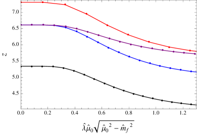
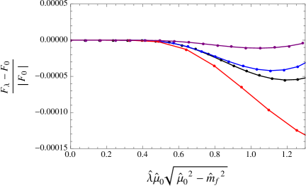
Figure 2: The near horizon Lifshitz scaling exponent $z$ and the relative free energy $\big{(}F_{\hat{\lambda}}-F_{0}\big{)}/|F_{0}|$, with $F_{0}$ the free energy of the $\lambda=0$ electron star, as a function of the dimensionless coupling constant $\lambda\nu_{0}$ for different parameters: $\hat{m}_{f}=0.2,c=1/3,\beta=5~{}(\text{Blue})$, $\hat{m}_{f}=0.3,c=1/3,\beta=5~{}(\text{Red})$; $\hat{m}_{f}=0.2,c=1/4,\beta=5~{}(\text{Purple})$; $\hat{m}_{f}=0.2,c=1/3,\beta=6~{}(\text{Black})$. For $\hat{\lambda}\hat{\mu}_{0}\sqrt{\hat{\mu}_{0}^{2}-\hat{m}_{f}^{2}}\lower 2.90623pt\hbox{$\sim$}\hbox to0.0pt{\hss\raise 1.04625pt\hbox{$<$}}1$ the free energy shows that the BCS star is the preferred groundstate. The rising free energy beyond $\hat{\lambda}\hat{\mu}_{0}\sqrt{\hat{\mu}_{0}^{2}-\hat{m}_{f}^{2}}=1$ should not be trusted. This is where perturbation theory breaks down.

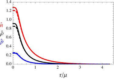
Figure 3: The BCS star profile as a function of the radial coordinate for $\hat{m}_{f}=0.2,c=1/3,\beta=5$ and $\hat{\lambda}\hat{\mu}\sqrt{\hat{\mu}^{2}-\hat{m}_{f}^{2}}=$ 0.649. Left: from top to bottom the fluid densities $\hat{n}_{f}$,$\hat{\rho}_{f}$,$\hat{p}_{f}$ of the BCS star (solid line) compared to the electron star (with same $\hat{m}_{f},\beta$ and $\hat{\lambda}\hat{\mu}\sqrt{\hat{\mu}^{2}-\hat{m}_{f}^{2}}=0$; dashed line). Both the charge(number) and energy density increase compared to the electron star. The star edges $r_{s}/\mu$ for ES and BCS are 4.320 and 4.329 respectively. Right: the order parameter $\hat{\Delta}$ in the BCS star solution.

III Properties of the dual field theory: evidence of superconductivity

In the last section we showed that our BCS star is more stable than the electron star solution at zero temperature and nonzero $\lambda$ and it can be seen as a continuous interaction driven quantum phase transition at $T=0$. In this section we will show the evidence that this BCS star corresponds to a superconducting state at the boundary. We cannot show this by conventional holographic means. Due to the fact that no collective fields extend beyond edge of the star — an artifact of the Thomas-Fermi approximation — there is no leading coefficient to be read off near the AdS boundary. Instead we will first show that there is a gap in the dual Fermi spectral function which resembles that of a superconducting state. Next we will study the change in the constituent charge densities, and show explicitly that charge disappears from the Fermi liquid into the bosonic sector. This shows that Cooper pairs have formed and have carried away the charge. Finally we compute the conductivity at small frequency and show that it has the hallmark characteristics of a holographic superconductor: a delta-function peak at zero frequency (foremost a consequence of momentum conservation) and a soft gap at $\omega<\Delta$.

III.1 Gap in the Fermi spectral function

To calculate the dual Fermi spectral function, we need to consider Fermi perturbations in the bulk which couple to the local gap function $\Delta$ with a BCS interaction as follows:

$$S_{\text{probe}}=\int d^{4}x\sqrt{-g}\bigg{[}-i\bar{\Psi}(\Gamma^{\mu}\mathcal{D}_{\mu}-m_{f})\Psi+\frac{1}{2}\Delta^{*}\bar{\Psi}_{c}\Gamma^{5}\Psi-\frac{1}{2}\Delta\bar{\Psi}\Gamma^{5}\Psi_{c}\bigg{]}.$$ (57)

The probe fermion has the same mass and charge as the fermion that constitute the bulk star solution before the scaling. The scaling, however, does not act uniformly on the probes Cubrovic:2011xm . After the scaling, an explicit dependence on the ratio $L/\kappa$ remains. This is the reflection of the inherent quantum mechanical nature of fermions. We will not consider this in detail because these coefficients are not important for showing the physical results related to the gap.

The BCS interaction term couples two modes of opposite spin, which have the same spectrum. The gap in the fermion spectrum is simply the level repulsion from coupling two degenerate states. The Dirac equation with BCS interaction is

$$i(\Gamma^{\mu}D_{\mu}-m_{f})\Psi+\Delta\Gamma^{5}\Psi_{c}=0.$$ (58)

After rescaling

$$\psi=(-gg^{rr})^{1/4}\Psi,$$ (59)

we have

$$(\Gamma^{r}\partial_{r}+\Gamma^{\mu}k_{\mu}-m_{f})\psi(r,k,\omega)-\Delta C\Gamma^{5}\Gamma^{0}\psi^{*}(r,-k,-\omega)=0$$ (60)

in the momentum space. Using

$$\psi=(\psi_{1},\psi_{2})^{T},$$ (61)

equation (60) can be written as

$$\big{(}-\sqrt{g^{rr}}\sigma^{3}\partial_{r}\mp i\sqrt{g^{xx}}\sigma^{2}k+(\omega+A_{t})\sqrt{g^{tt}}\sigma^{1}-m_{f}\big{)}\psi_{1,2}(r,k,\omega)\pm i\Delta\sigma^{1}\psi_{2,1}^{*}(r,-k,-\omega)=0$$ (62)

from which we observe $\psi_{1}(r,k,\omega)$ is coupled to $\psi_{2}^{*}(r,-k,-\omega)$ and $\psi_{2}(r,k,\omega)$ is coupled to $\psi_{1}^{*}(r,-k,-\omega)$. From the free Dirac equation of motion we can see that the spectrum of $\psi_{1}(r,k,\omega)$ and $\psi_{2}^{*}(r,-k,-\omega)$ are the same at $\omega=0$. This is the degenerate point where the BCS interaction couples causes a gap.

To calculate the dual Green's function, we should first specify the near horizon boundary conditions for this system. Following Faulkner:2009am ; Liu:2012tr , we treat the BCS coupling term as a perturbation. This is consistent since both at the horizon and at the boundary, $\Delta$ is finite, so the interaction term is sub-leading compared to other terms. At the horizon we must choose infalling boundary conditions to obtain the retarded Green's function in the dual boundary theory. They can be chosen independently for $\psi_{1}(r,k,\omega)$ and $\psi_{2}^{*}(r,-k,-\omega)$. To solve the system, we can chose as a basis the linearly independent choice I where $\psi_{1}(r,k,\omega)=0$, $\psi_{2}^{*}(r,-k,-\omega)$ is ingoing and choice II where $\psi_{1}(r,k,\omega)$ is ingoing while $\psi_{2}(r,-k,-\omega)=0$. Solving the Dirac equation with these two independent horizon boundary conditions, we obtain two sets of values at the AdS boundary at $r=\infty$. As the BCS coupling is again subleading, the general form of the boundary behavior is

$$\psi_{1}^{\text{I,II}}(k,\omega)=A_{1}^{\text{I,II}}r^{m}\begin{pmatrix}0\\ 1\end{pmatrix}+B_{1}^{\text{I,II}}r^{-m}\begin{pmatrix}1\\ 0\end{pmatrix}$$ (63)

and

$$\psi_{2}^{*\text{I,II}}(-k,-\omega)=A_{2}^{*\text{I,II}}r^{m}\begin{pmatrix}0\\ 1\end{pmatrix}+B_{2}^{*\text{I,II}}r^{-m}\begin{pmatrix}1\\ 0\end{pmatrix}.$$ (64)

where the superscript I,II refers to the choice of horizon boundary conditions.

We therefore obtain a matrix of responses $B$ to the various sources $A$,

$$\begin{pmatrix}B_{1}^{\text{I}}&B_{1}^{\text{II}}\\ B_{2}^{*\text{I}}&B_{2}^{*\text{II}}\end{pmatrix}=\begin{pmatrix}G_{O_{1}O_{1}^{\dagger}}&G_{O_{1}O_{2}}\\ G_{O_{2}^{\dagger}O_{1}^{\dagger}}&G_{O_{2}^{\dagger}O_{2}}\end{pmatrix}\begin{pmatrix}A_{1}^{\text{I}}&A_{1}^{\text{II}}\\ -A_{2}^{*\text{I}}&-A_{2}^{*\text{II}}\end{pmatrix}.$$ (65)

The Green's function can then be calculated as $G=BA^{-1}.$ In the absence of a BCS interaction $G$ is diagonal. In the perturbative limit we use here, the off-diagonal terms are of order $\Delta$ and the diagonal terms receive corrections of order $\Delta^{2}$.

In the absence of the BCS interaction, the system has poles at $\omega=0$ and we can define the (set of) Fermi momentum(momenta) $k_{F}$ as the value(s) where the leading fall-off of the (diagonal) solution vanishes $A_{1}^{\text{I}}(k_{F},0)=0$ and $A_{2}^{*\text{II}}(-k_{F},0)=0$. For a star solution which exists in the WKB limit, there are usually multiple Fermi surfaces Hartnoll:2011dm ; Iqbal:2011in ; Cubrovic:2011xm . Here we take $k_{F}$ to be the largest Fermi surface — the primary Fermi surface — though the following arguments apply to any of the Fermi surfaces.

Including now the BCS interaction, the source matrix $A$ near $(k=k_{F},\omega=0)$ is

$$A(k_{F},\omega)\sim\begin{pmatrix}a_{1}^{\text{I}}\omega&a_{1}^{\text{II}}\Delta\\ -a_{2}^{*\text{I}}\Delta&-a_{2}^{*\text{II}}\omega\end{pmatrix}+{\cal O}(\Delta^{2},\omega^{2})$$ (66)

at the leading order, where $a_{1}^{\text{I,II}}$ and $a_{2}^{*\text{I,II}}$ are constants of order $\mathcal{O}(1)$ near the Fermi surface. From this expression we can already see that there is a gap at the Fermi surface with size $\Delta$. In Faulkner:2009am , these coefficients are obtained explicitly by expanding the system near $\omega=0$ and at $k=k_{F}$. Denoting the (normalizable) solution to the Dirac equations for which $A(k,\omega)$ vanishes at $\omega=0$ and $k=k_{F}$ as $\psi_{1}^{\text{I}}(k_{F},0)=\xi_{1}^{(0)}$ and $\psi_{2}^{*\text{II}}(-k_{F},0)=\xi_{2}^{(0)}$, they find Faulkner:2009am :

$$G_{R}^{-1}(k_{F},\omega)\sim\begin{pmatrix}\omega P_{1}&Q_{1}\\ Q_{2}&\omega P_{2}\end{pmatrix},$$ (67)

where

$$P_{\alpha} = \int dr\sqrt{g_{rr}}\bar{\xi}_{\alpha}^{(0)}\sqrt{g^{tt}}\xi_{\alpha}^{(0)}(-1)^{\alpha},$$

$$Q_{1} = \int dr\sqrt{g_{rr}}\bar{\xi_{1}}^{(0)}i\Delta\xi_{2}^{(0)},$$ (68)

$$Q_{2} = \int dr\sqrt{g_{rr}}\bar{\xi_{2}}^{(0)}i\Delta\xi_{1}^{(0)}.$$

Diagonalizing one finds a gap for

$$|\omega|<\sqrt{Q_{1}Q_{2}/P_{1}P_{2}}$$ (69)

which is of order $\Delta$ taking value at the horizon. This gap in the fermion spectral function indicates that the field theory should be in a superconducting state. Similar to the holographic lattice gap Liu:2012tr , this gap is only a pseudo-gap in the sense that the $G^{-1}_{R}$ is only zero at one special $\omega$ and away from that frequency there will be small spectral weights.

III.2 Superconductivity induced changes in the charge density

The gap in the spectral function of the dual CFT on the boundary is the consequence of the superconducting core in the BCS star, even though its wavefunction does not extend to boundary. It is readily understood why: the lifting of the degeneracy need only to happen at one point in the interior. Another effect that persists into the dual CFT is the redistribution of the charge density of the system. The boundary charge density arises from the boundary value of the Maxwell field and when there is no contribution of charge density from inside the horizon, the boundary charge density is also equal to the integration of the bulk charge density along the radial direction Iqbal:2011bf ; Hartnoll:2011dm . Assuming that all fermions in region II immediately pair up at any finite $\lambda$, we can separate the total boundary charge density into two parts: the free charge density $Q_{\text{free}}$ from the fermions in region I, and the charge density which corresponds to paired fermions $Q_{\text{pair}}=Q_{\text{total}}-Q_{\text{free}}$ in the bulk. They can be obtained by the bulk integration of the charge density as follows

$$Q_{\text{free}}=\int_{0}^{r_{s}}drr^{2}\sqrt{g_{rr}}n_{\text{I}}^{\text{FL}},~{}~{}~{}~{}Q_{\text{total}}=\int_{0}^{r_{s}}drr^{2}\sqrt{g_{rr}}n,$$ (70)

with $n_{\text{I}}^{\text{FL}}$ in (13).

A further quantity of interest is the deviation from the exact equation of state of the free Fermi liquid. This is qualitatively captured by the amount of charge in the deviation density

$$Q_{\text{dev}}=\int_{0}^{r_{s}}drr^{2}\sqrt{g_{rr}}\delta n_{\text{total}}$$ (71)

with $\delta n_{\text{total}}$ in (42).

In Fig. 4, we show both the absolute and relative values of these charge density contributions compared to the total charge $Q_{\text{total}}$ as a function of the BCS coupling $\lambda$. Perhaps counterintuitively, the total charge density $Q_{\text{total}}$ (in units of the chemical potential $\mu$) decreases as we increase the BCS coupling $\hat{\lambda}\hat{\nu}_{0}$. It is known in condensed matter physics that the charge density is generically influenced by the condensate when the normal state is not invariant under charge conjugation on the scale of the superconducting gap. In weak coupling BCS it can be calculated that the charge density changes with a difference proportional to the order of the gap, but because it is weakly coupled the gap is small enough for this difference to be ignored. However, when the superconductor gets more strongly coupled such that the density of states is asymmetric around the Fermi surface on the scale of the gap the charge density (or either the chemical potential in the case of the grand canonical ensemble) changes when the order parameter develops. A typical example of the consequences of this very basic property is that vortices (where the core turns normal) are charged in more strongly coupled superconductors as confirmed by experiments in high Tc superconductors Feiner ; Khomskii . Here in our holographic model the decrease shows that the interaction makes charged excitations more difficult to populate rather than easier. Part of this decrease is simply due to Bose-Fermi competition: we see this as the decreasing contribution from the free fermions in region I. Condensing Cooper pairs do compensate this decrease, but not sufficiently so to increase $Q_{\text{total}}$. The fact that Cooper pairs do form is shown by the non-vanishing deviation from the Fermi liquid equation of state $Q_{\text{dev}}$. The non-vanishing charge density in the Cooper-pair sector shows explicitly that the dual ground state is charged and breaks the $U(1)$ gauge symmetry.

Note that our definition of $Q_{\text{free}}$ only counts the fermions in region I. Therefore it does not equal $Q_{\text{total}}=Q_{\text{I}}+Q_{\text{II}}$ at $\lambda=0$.

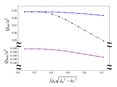
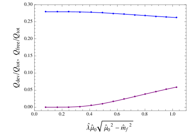
Figure 4: The total and free fermion charge density, $Q_{\text{total}}$ and $Q_{\text{free}}$ as a function of $\hat{\lambda}\hat{\mu}_{0}\sqrt{\hat{\mu}_{0}^{2}-\hat{m}_{f}^{2}}$ for $\hat{m}_{f}=0.2,c=1/3,\beta=5$. The dashed (black) line in the left figure between $Q_{\text{free}}$ and $Q_{\text{total}}$ shows the effect of the change of the equation of state compared to the standard free Fermi liquid: it is the contribution $Q_{\text{dev}}$. The decrease in the free fermion contribution is compensated by the change in the equation of state. but only partially. Note that $Q_{\text{total}}$ decreases as a function of the coupling $\lambda\nu_{0}$ indicating that it becomes progressively more difficult to excite charged carriers as the BCS coupling is turned on. On the right hand side we show the relative contributions $Q_{\text{free}}/Q_{\text{total}}$, $Q_{\text{dev}}/Q_{\text{total}}$. This visibly shows the pairing taking place as the deviation from the free Fermi liquid equation of state grows.

III.3 Conductivity at low frequency

For completeness, we also consider the behavior of conductivity at low frequency for the dual field theory. Following Hartnoll:2010gu , we consider the time dependent perturbations:

$$A_{x}=\frac{eL}{\kappa}\delta a_{x}(r)e^{-i\omega t},~{}~{}g_{tx}=L^{2}\delta g_{tx}(r)e^{-i\omega t},~{}~{}u_{x}=L\delta u_{x}(r)e^{-i\omega t}.$$ (72)

The equations of motion for these fluctuations are

$$\hat{n}\delta a_{x}+(\hat{\rho}+\hat{p})\delta u_{x} = 0,$$

$$\delta g_{tx}^{\prime}-\frac{2}{r}\delta g_{tx}+2h^{\prime}\delta a_{x} = 0,$$ (73)

$$\delta a^{\prime\prime}_{x}+\frac{1}{2}\bigg{(}\frac{f^{\prime}}{f}-\frac{g^{\prime}}{g}\bigg{)}\delta a^{\prime}_{x}+\omega^{2}\frac{g}{f}\delta a_{x}+\frac{h^{\prime}}{f}\bigg{(}\delta g^{\prime}_{tx}-\frac{2}{r}\delta g_{tx}\bigg{)}+g\hat{n}\delta u_{x} = 0.$$

Substituting the first and second equations in (73) into the third, we obtain the EOM for $\delta a_{x}$

$$\delta a^{\prime\prime}_{x}+\frac{1}{2}\bigg{(}\frac{f^{\prime}}{f}-\frac{g^{\prime}}{g}\bigg{)}\delta a^{\prime}_{x}+\bigg{(}\frac{g\omega^{2}}{f}-\frac{2h^{\prime 2}}{f}-\frac{g\hat{n}^{2}}{\hat{\rho}+\hat{p}}\bigg{)}\delta a_{x}=0.$$ (74)

The near horizon geometry of the BCS star is a Lifshitz geometry controlled by the dynamical critical exponent $z$ and the solution of (74) in the Lifshitz region with the infalling boundary condition $\delta a_{x}^{(\text{in})}\sim e^{i\frac{\omega\sqrt{g_{0}}}{zr^{z}}}$ is

$$\delta a_{x}=\sqrt{\omega}r^{-\frac{z}{2}}H^{(1)}_{\frac{\sqrt{4c_{0}+z^{2}}}{2z}}\bigg{[}\frac{\sqrt{g_{0}}\omega r^{-z}}{z}\bigg{]}.$$ (75)

Here the freedom to set the amplitude in the fluctuation equation is used to set it proportional to $\sqrt{\omega}$ — this way the leading order coefficient for the near-horizon infalling wave does not depend on frequency, $H^{(1)}_{\nu}(x)$ is the Hankel function of first kind and the constant $c_{0}$ equals

$$c_{0}=2h_{0}^{2}z^{2}+\frac{g_{0}\beta}{h_{0}}\bigg{(}\frac{1}{3}(h_{0}^{2}-m^{2})^{3/2}+\frac{2h_{0}^{2}-m^{2}}{h_{0}(h_{0}^{2}-m^{2})}\frac{\Delta_{0}^{2}}{\lambda}\bigg{)}.$$ (76)

Substituting in the the relations between $g_{0},h_{0},\Delta_{0}$ and $z$ from the near horizon EOM, it is easy to show that $c_{0}=2z^{2}$ and does not depend on the BCS coupling $\lambda$. Hence index of the Hankel function is just $3/2$.

Near the AdS₄ boundary, on the other hand, we have

$$\delta a_{x}=\delta a_{x}^{(0)}+\frac{\delta a_{x}^{(1)}}{r}+\dots,$$ (77)

The conductivity for the dual field theory is extracted from these values as

$$\sigma=-\frac{i}{\omega}\frac{\delta a_{x}^{(1)}}{\delta a_{x}^{(0)}}.$$ (78)

For low frequencies the near AdS₄ boundary coefficients can be related to the near horizon behavior through the conserved quantity Hartnoll:2010gu

$$\mathcal{F}=i\sqrt{\frac{f}{g}}\bigg{(}\delta a_{x}^{*}\partial_{r}\delta a_{x}-\delta a_{x}\partial_{r}\delta a_{x}^{*}\bigg{)}.$$ (79)

Near the AdS₄ boundary ${\cal F}$ equals $\mathcal{F}=-2\omega|\delta a_{x}^{(0)}|^{2}\text{Re}\sigma$, whereas the near horizon solution (75) gives $\mathcal{F}\sim\omega$. Thus $\text{Re}\sigma\sim|\delta a_{x}^{(0)}|^{-2}$. Using the matching method it is then easy to see $|\delta a_{x}^{(0)}|\propto\omega^{-1}$ Hartnoll:2010gu . Thus the low frequency behavior of the conductivity is

$$\text{Re}~{}\sigma\propto\delta(\omega)+\omega^{2}.$$ (80)

Notice that the delta function has to be there due to the translation invariance of the BCS star background. In more detail, this arises from the pole in the conductivity when $\omega\to 0$, as can be verified by evaluating (78) explicitly.

The small frequency behavior of the conductivity is in fact independent of the BCS coupling $\lambda$, since the computation is in this regard tracks not different from the computation for the electron star with $\lambda=0$. This hard gap is also missing in the holographic superconductor Gubser:2009cg ; Horowitz:2009ij . This is understood as a remnant effect of the near-horizon Lifshitz geometry. Since the geometry persists all the way to $r\rightarrow 0$, in the dual field theory there are a ``large $N$'' amount of degrees of freedom surviving in the IR. These coexists with the phase mode of the superconductor, causing the remnant finite conductivity in the region where which would be fully gapped in a conventional superconductor.

IV Scaling limits with a dynamical scalar

In our BCS star model, the matter fields are not visible at the boundary, though in the last section we showed that there are still effects on the boundary theory. Here we study a more generalized model which includes dynamics for the scalar field $\Delta$. Technically this will allow $\Delta$ to extend all the way to boundary. Physically, from the pure BCS perspective, this may seem strange. Indeed the most natural way to interpret the dual field theory this model describes, is as a system with charged fermions and an additional independent charged scalar operator with charge $q_{b}=2q_{f}$. From the gravity perspective, however, it is a very natural description that arises in many top-down models.

IV.1 Lagrangian with a dynamical scalar

In Liu:2013yaa we considered models with both dynamical scalars and fermions. There we found that the holographic description of strongly coupled systems with both bosons and fermions with incommensurate charges $q_{b}\neq 2nq_{f},~{}n\in\mathbb{N}$, has electron star solutions which can coexist with scalar hair (see also Nitti:2013xaa ). This corresponds to a superconducting state with multiple Fermi surfaces. In that case the incommensurate charge prevents a relation between the fermions and bosons in the gravitational bulk, and hence in the boundary.

A commensurate scalar charge $q_{b}=2q_{f}$ allows a Yukawa/BCS interaction between fermions and bosons in the bulk. This is what we studied so far, but without explicit dynamics for the scalar field. It only arose as an auxiliary field. For a dynamical scalar, on the other hand, it is natural to surmise that the energetics of the bosons can be relevant to the condensation of the fermions. The more generalized system we therefore consider is

$$\mathcal{L} = \frac{1}{2\kappa^{2}}\bigg{(}R+\frac{6}{L^{2}}\bigg{)}-\frac{1}{4e^{2}}F_{\mu\nu}F^{\mu\nu}-|(\partial_{\mu}-2iqA_{\mu})\phi|^{2}-m_{\phi}^{2}|\phi|^{2}$$ (81)

$$-i\bar{\Psi}(\Gamma^{\mu}\mathcal{D}_{\mu}-m_{\Psi})\Psi+\eta_{5}^{*}\phi^{*}\bar{\Psi}_{c}\Gamma^{5}\Psi-\eta_{5}\phi\bar{\Psi}\Gamma^{5}\Psi_{c}.$$

This model has been considered before in Faulkner:2009am from a perspective where the fermions are probes, whereas $\eta_{5}=0$ this is a special case of the bose-fermi competition models studied in Liu:2013yaa ; Nitti:2013xaa with $q_{b}=2q_{f}$. Its connection to the BCS Lagrangian studied here is made clear after the field redefinition

$$\phi=\frac{1}{m_{\phi}\sqrt{2\lambda}}\Delta,~{}~{}~{}\eta_{5}=m_{\phi}\sqrt{\frac{\lambda}{2}}.$$ (82)

Then the Lagrangian becomes:

$$\mathcal{L} = \frac{1}{2\kappa^{2}}\bigg{(}R+\frac{6}{L^{2}}\bigg{)}-\frac{1}{4e^{2}}F_{\mu\nu}F^{\mu\nu}-\frac{1}{2\lambda m_{\phi}^{2}}|(\partial_{\mu}-2iqA_{\mu})\Delta|^{2}-\frac{1}{2\lambda}|\Delta|^{2}$$ (83)

$$-i\bar{\Psi}(\Gamma^{\mu}\mathcal{D}_{\mu}-m_{f})\Psi+\frac{1}{2}\Delta^{*}\bar{\Psi}_{c}\Gamma^{5}\Psi-\frac{1}{2}\Delta\bar{\Psi}\Gamma^{5}\Psi_{c}.$$

In the formal limit $m_{\phi}^{2}\rightarrow\infty$ we recover the Einstein-Maxwell-BCS Lagrangian. We will now make this limit more precise.

The equations of motion for this system are

$$R_{\mu\nu}-\frac{1}{2}g_{\mu\nu}R-\frac{3}{L^{2}}g_{\mu\nu}-\kappa^{2}\bigg{[}T_{\mu\nu}^{\text{gauge}}+T_{\mu\nu}^{\text{BCS}}\bigg{]} = \kappa^{2}\bigg{[}T_{\mu\nu}^{\text{kin.boson}}\bigg{]};$$

$${\nabla_{\mu}}F^{\mu\nu}+e^{2}J^{\nu}_{\text{BCS}} = \frac{iqe^{2}}{\lambda m_{\phi}^{2}}\bigg{[}\Delta^{*}\big{(}\partial^{\nu}-2iqA^{\nu}\big{)}\Delta-\Delta\big{(}\partial^{\nu}+2iqA^{\nu}\big{)}\Delta^{*}\bigg{]};$$

$$\Delta-\lambda\bar{\Psi}_{c}\Gamma^{5}\Psi = \frac{1}{m_{\phi}^{2}}\big{(}\nabla^{\mu}-2iqA^{\mu}\big{)}\big{(}\nabla_{\mu}-2iqA_{\mu}\big{)}\Delta;$$ (84)

$$i\big{(}\Gamma^{\mu}\mathcal{D}_{\mu}-m_{f}\big{)}\Psi-\Delta^{\dagger}\Psi_{c}\Gamma^{5}\Psi = 0,$$

where $T_{\mu\nu}^{\text{gauge}}$, $T_{\mu\nu}^{\text{BCS}}$ and $J^{\mu}_{\text{BCS}}$ are as before in Eqns (8) and (40), and

$$T_{\mu\nu}^{\text{kin.boson}} = \frac{1}{\lambda m_{\phi}^{2}}\bigg{(}\big{(}\partial_{(\mu}+2iqA_{(\mu}\big{)}\Delta^{*}\big{(}\partial_{\nu)}-2iqA_{\nu)}\big{)}\Delta-\frac{1}{2}g_{\mu\nu}|\big{(}\partial_{\alpha}-2iqA_{\alpha}\big{)}\Delta|^{2}\bigg{)},$$ (85)

with $A_{(\mu}B_{\nu)}=\frac{1}{2}(A_{\mu}B_{\nu}+A_{\nu}B_{\mu})$. The terms on the right hand side of (84) are new compared to the pure BCS system considered before. The decoupling limit needs more in depth inquiry, because we first need to impose a well-defined semi-classical limit for the many body fermion system. Making the fluid approximation $T_{\mu\nu}^{\text{BCS}}=(\rho+p)u_{\mu}u_{\nu}+pg_{\mu\nu}$ as in (40), this is obtained in terms of the dimensionless variables found earlier

$$(\rho,p)=\frac{1}{\kappa^{2}}(\hat{\rho},\hat{p}),~{}~{}~{}n=\frac{1}{e\kappa}\hat{n},~{}~{}~{}(A_{\mu},\mu_{l},m_{f},\Delta,\omega_{D})=\frac{e}{\kappa}(\hat{A}_{\mu},\hat{\mu},\hat{m}_{f},\hat{\Delta},\hat{\omega}_{D}),~{}~{}~{}\lambda=\frac{e^{2}}{\beta}\hat{\lambda}$$ (86)

where the hatted quantities are of order zero in $\kappa$ and $e$ with $\beta=e^{4}/\pi^{2}\kappa^{2}$ fixed, and for simplicity we have set $L=1$ and $q=1$ as $q$ only appears in the combination $qe$. In terms of the rescaled variables the bosonic EOM become

$$R_{\mu\nu}-\frac{1}{2}g_{\mu\nu}R-3g_{\mu\nu}-\bigg{[}\hat{T}_{\mu\nu}^{\text{gauge}}+\hat{T}_{\mu\nu}^{\text{BCS}}\bigg{]} = \frac{\beta}{\hat{\lambda}m_{\phi}^{2}}\bigg{[}(\partial_{(\mu}+2i\frac{q_{\text{eff}}}{\sqrt{\kappa}}\hat{A}_{(\mu})\hat{\Delta}^{*}(\partial_{\nu)}-2i\frac{q_{\text{eff}}}{\sqrt{\kappa}}\hat{A}_{\nu)})\hat{\Delta}$$

$$~{}~{}~{}-\frac{1}{2}g_{\mu\nu}|\big{(}\partial_{\alpha}-2i\frac{q_{\text{eff}}}{\sqrt{\kappa}}\hat{A}_{\alpha}\big{)}\hat{\Delta}|^{2}\bigg{]};$$

$${\nabla_{\mu}}\hat{F}^{\mu\nu}+\hat{J}^{\nu}_{\text{BCS}} = \frac{e}{\kappa}\frac{i\beta}{\hat{\lambda}m_{\phi}^{2}}\bigg{[}\hat{\Delta}^{*}(\partial^{\nu}-2i\frac{q_{\text{eff}}}{\sqrt{\kappa}}\hat{A}^{\nu})\hat{\Delta}-\hat{\Delta}(\partial^{\nu}+2i\frac{q_{\text{eff}}}{\sqrt{\kappa}}\hat{A}^{\nu})\hat{\Delta}^{*}\bigg{]};$$

$$\hat{\Delta}-\hat{\lambda}\langle\bar{\Psi}_{c}\Gamma^{5}\Psi\rangle = \frac{1}{m_{\phi}^{2}}(\nabla^{\mu}-2i\frac{q_{\text{eff}}}{\sqrt{\kappa}}\hat{A}^{\mu})(\nabla_{\mu}-2i\frac{q_{\text{eff}}}{\sqrt{\kappa}}\hat{A}_{\mu})\hat{\Delta},$$ (87)

where $q_{\text{eff}}=\sqrt{\pi}\beta^{1/4}$.

We see that there is no clean classical gravity limit $\kappa\to 0$, where the rescaled fields can stay fixed and the energy momentum contribution to the gravity is still of order $\mathcal{O}(1)$. This is precisely due to the fact that the bosonic charge is fixed in units of the fermion charge. For incommensurate charges, i.e. if $q_{\text{eff}}$ were a free parameter, one can scale this charge to absorb the explicit dependence on the gravitational coupling $\kappa$; see Liu:2013yaa . The fact that the fluid limit is incompatible with a scaling limit in the microscopic Lagrangian was already noted in Cubrovic:2011xm .

In our case, where $q_{b}$ is not free, but fixed to equal $q_{b}=2q_{f}$, there are three possible classical limits. They depend on the scaling choice for the mass $m_{\phi}$. One has:

• $m_{\phi}^{2}=\kappa^{-1-\delta}\hat{m}_{\phi}^{2}$ where $\delta>0$: This is the limit where the kinetics of the scalar completely decouples and one recovers the system studied in the previous sections.

• $m_{\phi}^{2}=\kappa^{-1}\hat{m}_{\phi}^{2}$. This is the natural limit in which the hatted parameter $m_{\phi}^{2}$ is a truly dimensionless parameter. In this limit the strict kinetics of the scalar field are unimportant, but the coupling to the gauge field and to the fermionic field remain. This is exactly the case we will study in this section.

• $m_{\phi}^{2}=\kappa^{-1-\delta}\hat{m}_{\phi}^{2}$ where $\delta<0$. This is not a well defined classical limit which means the scaling (86) could be modified resulting in that not all fermionic terms could be kept. Applying it nevertheless means that the kinetics of the scalar field can be kept and dominate but its derivative decouples from the Maxwell connection. In essence $q_{\text{eff}}$ must be set to zero. We leave this case for future study.

IV.2 Charged non-dynamical scalar scaling limit

We now focus on the second case where $m_{\phi}^{2}=\kappa^{-1}\hat{m}_{\phi}^{2}$ and take the limit $\kappa\rightarrow 0$ with all hatted quantities fixed. The ansatz for the background we take is the same as (46). We now define a new combined fluid

$$T_{\mu\nu}^{\text{BCS}}+T_{\mu\nu}^{\text{kin.boson}}=(\rho_{\text{com}}+p_{\text{com}})u_{\mu}u_{\nu}+p_{\text{com}}g_{\mu\nu}$$

and

$$J_{\mu}^{\text{fermion}}+J_{\mu}^{\text{boson}}=n_{\text{com}}u_{\mu}$$

where the rescaled fluid quantities

$$\hat{\rho}_{\text{com}}=\hat{\rho}+\frac{s\beta h^{2}}{f}\frac{\hat{\Delta}^{2}}{\hat{\lambda}},~{}~{}~{}\hat{p}_{\text{com}}=\hat{p}+\frac{s\beta h^{2}}{f}\frac{\hat{\Delta}^{2}}{\hat{\lambda}},~{}~{}~{}\hat{n}_{\text{com}}=\hat{n}+\frac{2s\beta h}{\sqrt{f}}\frac{\hat{\Delta}^{2}}{\hat{\lambda}}$$ (88)

are the BCS fluid quantities in (40) and we have introduced the parameter $s$ related to the scalar mass for convenience

$$s\equiv\frac{2\pi\sqrt{\beta}}{\hat{m}_{\phi}^{2}}.$$ (89)

Obviously, when $s\to 0$, i.e. $\hat{m}_{\phi}^{2}\to\infty$, our system reduces to the BCS star system discussed in the previous section. For finite $s$ the equations of motion for the system in terms of the combined fluid are the same as the previous case, (II.2-48) with the exception of the equation of motion for the scalar field. It gives

$$-\frac{2sh^{2}}{f\hat{\lambda}}+\frac{1}{\hat{\lambda}}=\pi^{2}\int_{-\hat{\omega}_{D}}^{\hat{\omega}_{D}}d\xi\hat{\nu}(\xi)\frac{1}{\sqrt{\xi^{2}+\hat{\Delta}^{2}}}.$$ (90)

In the same limit as before ${\hat{\Delta}}\ll\hat{\omega}_{D}\ll(\hat{\mu},\hat{\mu}-\hat{m}_{f})$, this modified gap equation can be solved as

$$\hat{\Delta}=2\hat{\omega}_{D}e^{-(1-\frac{2sh^{2}}{f})/(\hat{\lambda}\hat{\mu}\sqrt{\hat{\mu}^{2}-\hat{m}_{f}^{2}})}.$$ (91)

From (91) it is easy to see when $s$ is large, $1-2sh^{2}/f$ would be negative and the approximation ${\hat{\Delta}}\ll\hat{\omega}_{D}$ would break down. Thus the perturbative approach we follow here only applies for small $s$.

Let us explain in more detail the way this system works in this limit, where especially the role of the scalar field equation is interesting. In this limit all kinetics decouple: the scalar field has become an auxiliary field again. However, we can see that $\Delta$ is no longer the Cooper pair condensate. Nevertheless, this gap is still associated with a local superconducting state in the bulk as can be seen from the Dirac equation. What is happening is that the charged gap field is now also sensitive to the background gauge connection. Note that it does do so in a way that gauge symmetry is broken. The gap field has the status of a Stueckelberg field. The limit is therefore a Stueckelberg limit where strict decoupling does not happen. Only at low energies, much below $m_{\phi}$, this is a reliable approximation to the system.

For the solution of this BCS-Stueckelberg system, we proceed as before. The near horizon geometry is still Lifshitz. One can add an irrelevant perturbation for the geometry to flow to an AdS solution. The behavior of the fluid and condensate is plotted in Fig. 6. The significant difference compared to the pure BCS star is the enhancement in the charge density (Fig. 6). In particular we see the BCS-Stueckelberg star is more susceptible to form a superconducting core. This can be directly understood from the reduced suppression of the gap. The stronger predilection towards pairing should also be reflected in the thermodynamic properties. Indeed the BCS-Stueckelberg star in this limit is more stable (Fig. 7).

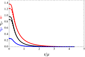
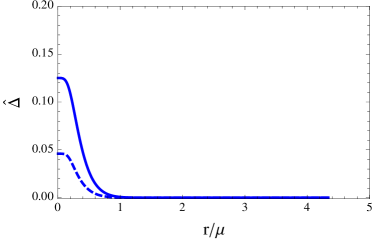
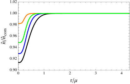
Figure 5: The profile for the fluid in the star in the BCS-Stueckelberg limit as a function of the radial coordinate with $\hat{m}_{f}=0.2,c=1/3,\beta=5$, $\hat{\lambda}\hat{\mu}\sqrt{\mu^{2}-\hat{m}_{f}^{2}}=$ 0.393. Left: from top to bottom, the solid lines are $\hat{n}_{\text{com}}$, $\hat{\rho}_{\text{com}}$, $\hat{p}_{\text{com}}$ with $s=0.25$ and the star edge $r_{s}/\mu\simeq 4.338$. For comparison, we also give the profiles of the pure BCS star $\hat{n}_{\text{tot}}$, $\hat{\rho}_{\text{tot}}$, $\hat{p}_{\text{tot}}$ with $s=0$ and the star edge $r_{s}/\mu\simeq 4.328$; Right: The value of the gap $\hat{\Delta}$ for $s=0.25$ (solid) and $s=0$ (dashed) for the same numerical parameters. Both the gap and the charge density are enhanced compared to the pure BCS star.

Figure 6: The ratio of the pure BCS charge density $\hat{n}$ to the combined BCS-Stueckelberg charge density $\hat{n}_{\text{com}}$ as a function the radial coordinate for different coupling constant $\lambda$ for $\hat{m}_{f}=0.2,c=1/3,\beta=5$ and $s=0.25$. In the figure, $\hat{\lambda}\hat{\mu}\sqrt{\mu^{2}-\hat{m}_{f}^{2}}=$ 0.245 (Orange), 0.393 (Green), 0.534 (Blue), 0.810 (Black).

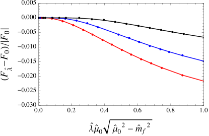
Figure 7: The near horizon Lifshitz scaling $z$ (left plot) and free energy (right plot) for the star in this new scaling limit as a function of $\lambda$ for $\hat{m}_{f}=0.2,c=1/3,\beta=5$ with different $s=0.25$ (black), $0.4$ (blue), $0.5$ (red). The free energy decreases as $\hat{\lambda}$ increases in the region that perturbation theory applies. The larger the Stueckelberg term, the more thermodynamically favored the solution is (and the smaller the IR dynamical critical exponent). This is in accordance with the corresponding increase in the gap.

The total charge distributions are also reflecting this extra stability. In the BCS-Stueckelberg star we can distinguish a third component contributing to the charge density: next to the free- and paired fermions there is also the contribution from the Stueckelberg field. Define a new combined charge density by

$$Q_{\text{com}}=\int_{0}^{r_{s}}drr^{2}\sqrt{g_{rr}}n_{\text{com}}$$ (92)

in addition to the densities $Q_{\text{free}}$ and $Q_{\text{total}}$ as given by (70). We can then define the Stueckelberg charge density as $Q_{\text{Stueck}}=Q_{\text{com}}-Q_{\text{total}}$. The left plot of Fig. 8 demonstrates that this extra Stueckelberg contribution gives rise to an increase of the charge density upon increasing the BCS coupling, as expected intuitively. Whereas the pure BCS contribution $Q_{\text{total}}$ decreases with increasing coupling as before, the extra Stueckelberg contribution suffices to compensate for the depletion of the free fermionic density, as illustrated in the right plot of Fig. 8.

Finally, we checked by explicit calculation along the lines of the previous section that the gap in the dual Fermion spectral function continues to be set by $\Delta$ also in this BCS-Stueckelberg limit. The novelty is just that the Stueckelberg field is enhancing this gap.

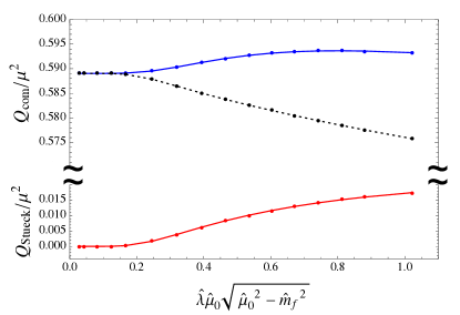
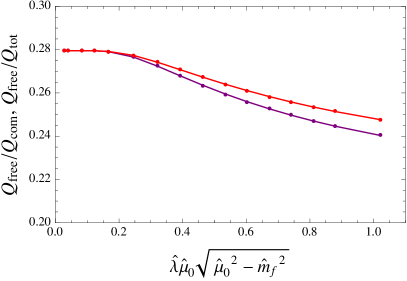
Figure 8: Left: The absolute charge densities $Q_{\text{com}}/\mu^{2}$ (blue), $Q_{\text{tot}}/\mu^{2}$ (black dashed) and $Q_{\text{Stueck}}/\mu^{2}$ (red) in the BCS-Stueckelberg star as a function of the coupling $\hat{\lambda}\hat{\mu}_{0}\sqrt{\hat{\mu}_{0}^{2}-\hat{m}_{f}^{2}}$. Right: The relative charge densities of $Q_{\text{free}}/Q_{\text{tot}}$ (red) and $Q_{\text{free}}/Q_{\text{com}}$ (purple) as a function of the coupling $\hat{\lambda}\hat{\mu}_{0}\sqrt{\hat{\mu}_{0}^{2}-\hat{m}_{f}^{2}}$ for $\hat{m}_{f}=0.2,c=1/3,\beta=5$ and $s=0.25.$

V Conclusion and discussion

In this paper we have made a step towards understanding fermion driven pairing in strongly coupled systems with holographic duals. In particular we considered the introduction of a BCS interaction for the fields dual to the fermionic operators in strongly coupled theory, i.e. we complemented the AdS-Einstein-Maxwell-Dirac action with a standard BCS interaction. This implicitly assumes that at low energies these fermionic operators control the physics and that the pairing is driven by a force other than the one that controls the strong correlations, even though this might be unnatural from more microscopic arguments or top-down AdS/CFT constructions; see e.g. erdmenger . Given this set up, however, we show that the holographic system does undergo spontaneous symmetry breaking that adheres closely to the BCS paradigm. We do so in a fluid limit for the many-body fermion system where we explicitly construct the BCS corrections to the fluid. The fluid limit has the advantage that we can compute the fully backreacted gravitational solution and hence understand the thermodynamic characteristics of the dual field theory. The symmetry breaking solution we find, therefore builds upon the Tolman-Oppenheimer-Volkov self-gravitating Fermi fluid solution underpinning neutron and electron stars. Indeed the BCS star is readily recognizable as an AdS electron star cousin of an astrophysical neutron star with a superconducting core. We show that at zero temperature and with a positive coupling, the corresponding BCS star solution is indeed the more stable groundstate than the pure electron star solution. As a function of the BCS coupling $\lambda$, the transition between the electron star and the BCS star can be seen as an interaction driven (continuous) quantum phase transition between the symmetry preserving state at $\lambda=0$ and the symmetry-broken state at $\lambda\neq 0$.

The symmetry breaking nature of the BCS star is confirmed by the appearance of a pseudo-gap in the Fermi spectral function of the boundary theory with the size of the gap is determined by the coupling constant. In addition the changes of the charge density at a fixed chemical potential for a BCS star solution implies the loss of charge in a superconducting state. Finally the conductivity is indeed suppressed at very low frequency, although as is characteristic of holographic superconductors, it does not exhibit a hard gap.

A primary motivation of our work is to build a realistic holographic superconductor in that it explicitly encodes the fermionic degrees of freedom present in real exotic superconductors. On the gravity side of the duality, we show that considerations of what is natural there, gives a novel Stueckelberg-like coupling of the gap field. Interestingly, in the resulting BCS-Stueckelberg star, the susceptibility of the system towards superconductivity is enhanced, even though the suppression of the gap remains exponential.

There are various avenues to pursue to make the system even more realistic. An obvious one is to consider lattice-effects and to encode the d-wave symmetry. In ordinary metals, the lattice phonons are responsible for the effective four point interaction of the fermions. It is likely that the same will happen in a holographic set-up with explicit fermions at finite density, as much of the fermionic physics follows the standard rules. In that sense our BCS study here carries few surprises, but it serves as another excellent benchmark of holographic duality. It also serves as stepping stone. Using this BCS star as a base, an inquiry that tries to connect it closer to the physics of strongly coupled physics that underly the AdS/CFT duality could provide genuinely new insights into the onset of superconductivity in quantum critical metals.

Appendix A Fluid parameters in region II

To obtain the result for the fluid parameters in region II quoted in Eqs. (32)-(34), one subtracts the free fermion contribution from region II, Eq. (35) from the formal expressions Eqs. (26), (27), and (II.1). Using the $\omega_{D}\ll\mu$ expansion for the density of states in these differences, one obtains the following expressions, where the the integrations can be performed explicitly.

$$n_{\text{II}}-n_{\text{II}}^{\text{FL}} \simeq\omega_{D}^{2}\nu_{1}-\int_{-\omega_{D}}^{\omega_{D}}d\xi\frac{\xi^{2}\nu_{1}}{\sqrt{\xi^{2}+\Delta^{2}}}$$

$$=-\nu_{1}\frac{\Delta^{2}}{2}+\nu_{1}\Delta^{2}\ln\frac{2\omega_{D}}{\Delta}~{},$$

$$\rho_{\text{II}}-\rho_{\text{II}}^{\text{FL}} \simeq(\omega_{D}^{2}-2\mu_{l}\omega_{D})\nu_{0}-(2\frac{\omega_{D}^{3}}{3}-\mu_{l}\omega_{D}^{2})\nu_{1}-\nu_{0}\int_{-\omega_{D}}^{\omega_{D}}d\xi{\sqrt{\xi^{2}+\Delta^{2}}}+\mu_{l}n_{\text{II}}+\rho_{\Delta}$$

$$=-(\nu_{0}+\mu_{l}\nu_{1})\frac{\Delta^{2}}{2}-(\nu_{0}-\mu_{l}\nu_{1})\Delta^{2}\ln\frac{2\omega_{D}}{\Delta}+\rho_{\Delta}~{},$$

$$p_{\text{II}}-p_{\text{II}}^{\text{FL}} \simeq\omega_{D}^{2}\nu_{0}-\frac{1}{3}\left[\nu_{1}\frac{\mu_{l}^{2}-m_{f}^{2}}{\mu}+\nu_{0}\left(\frac{-\mu_{l}^{2}+m_{f}^{2}}{\mu_{l}^{2}}+2\right)\right]\int_{-\omega_{D}}^{\omega_{D}}d\xi\frac{\xi^{2}}{\sqrt{\xi^{2}+\Delta^{2}}}+p_{\Delta}$$

$$=-\nu_{0}\frac{\Delta^{2}}{2}+\nu_{0}\Delta^{2}\ln\frac{2\omega_{D}}{\Delta}+p_{\Delta}~{}.$$ (93)

Expanding the integrated result in $\Delta\ll\omega_{D}$, while keeping the term $\rho_{\Delta}=-p_{\Delta}=\Delta^{2}/2\lambda$, one finds the expressions Eqs. (32)-(34).

References

• (1) H. Liu, J. McGreevy and D. Vegh, ``Non-Fermi liquids from holography,'' Phys. Rev. D 83, 065029 (2011) [arXiv:0903.2477 [hep-th]].
• (2) M. Cubrovic, J. Zaanen and K. Schalm, ``String Theory, Quantum Phase Transitions and the Emergent Fermi-Liquid,'' Science 325, 439 (2009) [arXiv:0904.1993 [hep-th]].
• (3) T. Faulkner, H. Liu, J. McGreevy and D. Vegh, ``Emergent quantum criticality, Fermi surfaces, and AdS(2),'' Phys. Rev. D 83, 125002 (2011) [arXiv:0907.2694 [hep-th]].
• (4) T. Faulkner and J. Polchinski, ``Semi-Holographic Fermi Liquids,'' JHEP 1106, 012 (2011) [arXiv:1001.5049 [hep-th]].
• (5) S. A. Hartnoll, C. P. Herzog and G. T. Horowitz, ``Building a Holographic Superconductor,'' Phys. Rev. Lett.  101, 031601 (2008) [arXiv:0803.3295 [hep-th]].
• (6) S. A. Hartnoll, C. P. Herzog and G. T. Horowitz, ``Holographic Superconductors,'' JHEP 0812, 015 (2008) [arXiv:0810.1563 [hep-th]].
• (7) J. -H. She, B. J. Overbosch, Y. -W. Sun, Y. Liu, K. Schalm, J. A. Mydosh and J. Zaanen, ``Observing the origin of superconductivity in quantum critical metals,'' Phys. Rev. B 84, 144527 (2011) [arXiv:1105.5377 [cond-mat.str-el]].
• (8) N. Iqbal, H. Liu and M. Mezei, ``Lectures on holographic non-Fermi liquids and quantum phase transitions,'' arXiv:1110.3814 [hep-th].
• (9) M. Ammon, J. Erdmenger, M. Kaminski and P. Kerner, ``Flavor Superconductivity from Gauge/Gravity Duality,'' JHEP 0910, 067 (2009) [arXiv:0903.1864 [hep-th]].
• (10) T. Faulkner, G. T. Horowitz, J. McGreevy, M. M. Roberts and D. Vegh, ``Photoemission `experiments' on holographic superconductors,'' JHEP 1003, 121 (2010) [arXiv:0911.3402 [hep-th]].
• (11) T. Hartman and S. A. Hartnoll, ``Cooper pairing near charged black holes,'' JHEP 1006, 005 (2010) [arXiv:1003.1918 [hep-th]].
• (12) A. Bagrov, B. Meszena and K. Schalm, ``Pairing induced superconductivity in holography,'' arXiv:1403.3699 [hep-th].
• (13) S. Sachdev, ``A model of a Fermi liquid using gauge-gravity duality,'' Phys. Rev. D 84, 066009 (2011) [arXiv:1107.5321 [hep-th]].
• (14) A. Allais, J. McGreevy and S. J. Suh, ``A quantum electron star,'' Phys. Rev. Lett.  108, 231602 (2012) [arXiv:1202.5308 [hep-th]].
• (15) A. Allais and J. McGreevy, ``How to construct a gravitating quantum electron star,'' Phys. Rev. D 88, 066006 (2013) [arXiv:1306.6075 [hep-th]].
• (16) J. Bardeen, L. N. Cooper, and J. R. Schrieffer, ``Theory of Superconductivity,'' Phys. Rev. 108, 1175 (1957).
• (17) D.  Bertrand, ``A Relativistic BCS Theory of Superconductivity,'' Ph.D. thesis,
Catholic University of Louvain (Louvain-la-Neuve, Belgium, July 2005), available at
http://https://cp3.irmp.ucl.ac.be/upload/theses/phd/bertrand.pdf
• (18) Y. Liu, K. Schalm, Y. -W. Sun and J. Zaanen, ``Bose-Fermi competition in holographic metals,'' JHEP 1310, 064 (2013) [arXiv:1307.4572 [hep-th]].
• (19) S. A. Hartnoll, J. Polchinski, E. Silverstein and D. Tong, ``Towards strange metallic holography,'' JHEP 1004, 120 (2010) [arXiv:0912.1061 [hep-th]].
• (20) J. de Boer, K. Papadodimas and E. Verlinde, ``Holographic Neutron Stars,'' JHEP 1010, 020 (2010) [arXiv:0907.2695 [hep-th]].
• (21) X. Arsiwalla, J. de Boer, K. Papadodimas and E. Verlinde, ``Degenerate Stars and Gravitational Collapse in AdS/CFT,'' JHEP 1101, 144 (2011) [arXiv:1010.5784 [hep-th]].
• (22) S. A. Hartnoll and A. Tavanfar, ``Electron stars for holographic metallic criticality,'' Phys. Rev. D 83, 046003 (2011) [arXiv:1008.2828 [hep-th]].
• (23) M. Cubrovic, Y. Liu, K. Schalm, Y. -W. Sun and J. Zaanen, ``Spectral probes of the holographic Fermi groundstate: dialing between the electron star and AdS Dirac hair,'' Phys. Rev. D 84, 086002 (2011) [arXiv:1106.1798 [hep-th]].
• (24) C. P. Herzog and J. Ren, ``The Spin of Holographic Electrons at Nonzero Density and Temperature,'' JHEP 1206, 078 (2012) [arXiv:1204.0518 [hep-th]].
• (25) V. Alexandrov and P. Coleman, ``Spin and holographic metals,'' Phys. Rev. B 86, 125145 (2012) [arXiv:1204.6310 [cond-mat.str-el]].
• (26) Y. Liu, K. Schalm, Y. -W. Sun and J. Zaanen, ``Lattice Potentials and Fermions in Holographic non Fermi-Liquids: Hybridizing Local Quantum Criticality,'' JHEP 1210, 036 (2012) [arXiv:1205.5227 [hep-th]].
• (27) S. A. Hartnoll, D. M. Hofman and D. Vegh, ``Stellar spectroscopy: Fermions and holographic Lifshitz criticality,'' JHEP 1108, 096 (2011) [arXiv:1105.3197 [hep-th]].
• (28) N. Iqbal, H. Liu and M. Mezei, ``Semi-local quantum liquids,'' JHEP 1204, 086 (2012) [arXiv:1105.4621 [hep-th]].
• (29) N. Iqbal and H. Liu, ``Luttinger's Theorem, Superfluid Vortices, and Holography,'' Class. Quant. Grav.  29, 194004 (2012) [arXiv:1112.3671 [hep-th]].
• (30) L. F. Feiner and J. Zaanen, ``Charged vortices in the negative U Hubbard model'', Physica C 162-164, 777 (1989).
• (31) D. I. Khomskii and A. Freimuth, ``Charged Vortices in High Temperature Superconductors'', Phys. Rev. Lett. 75, 1384 (1985).
• (32) S. S. Gubser and A. Nellore, ``Ground states of holographic superconductors,'' Phys. Rev. D 80, 105007 (2009) [arXiv:0908.1972 [hep-th]].
• (33) G. T. Horowitz and M. M. Roberts, ``Zero Temperature Limit of Holographic Superconductors,'' JHEP 0911, 015 (2009) [arXiv:0908.3677 [hep-th]].
• (34) F. Nitti, G. Policastro and T. Vanel, ``Dressing the Electron Star in a Holographic Superconductor,'' JHEP 1310, 019 (2013) [arXiv:1307.4558 [hep-th]].