ENERGY TERMS AND STABILITY
DIAGRAMS FOR THE 2$D$ PROBLEM
OF THREE CHARGED PARTICLES

Abstract

Symmetric and antisymmetric terms have been obtained in the framework of the variational approach for two-dimensional (2$D$) Coulomb systems of symmetric trions $XXY$.  Stability diagrams and certain anomalies arising in the 2$D$ space are explained qualitatively in the framework of the Born–Oppenheimer adiabatic approximation.  The asymptotics of energy terms at large distances obtained for an arbitrary space dimensionality are analyzed, and some approximation formulas for 2$D$ terms are proposed.  An anomalous dependence of multipole moments on the space dimensionality has been found in the case of a spherically symmetric field.  The main results obtained for the 2$D$ and 3$D$ problems of two Coulomb centers are compared.

1 Introduction

The two-dimensional (2$D$) problems for Coulomb systems arise in various physical domains: for layered and near-surface materials, in the physics of graphene, and in connection with general problems aimed at studying the dependences of physical observables on the space dimensionality (e.g., see works [1,​ 2]).  Researches of conditions required for the emergence of bound states in the 2$D$ problem of three charged particles and their comparison with those for the same problem in the three-dimensional (3$D$) space [3,​ 4] revealed certain important anomalies in the 2$D$ space, especially in the molecular mode [5].  Hence, there arises a necessity of a clearer, at the physical level, understanding of such two-dimensional features that are absent in the standard formulation of corresponding problems in the 3$D$ space.  In the molecular mode for a symmetric trion $XXY$ (in this case, we actually deal with two Coulomb centers), this 3$D$ problem has been studied rather completely (in particular, see works [6,​ 7,​ 8]).  For today, separate results for the asymptotics of energy terms at short and large distances have already been obtained for two Coulomb centers in the 2$D$ space as well [1,​ 2].  However, the application of these terms to studying the stability diagrams still requires a separate consideration.

In this work, the energy terms were calculated in the framework of a rather accurate variational approach and without separating the variables.  This technique can be extended to include more complicated systems.  Some approximation formulas for the terms are proposed with regard for the asymptotic formulas for large and short distances between the centers, and the features of the terms specific for various space dimensionalities are discussed.  The obtained terms are used to analyze the stability diagrams plotted in the mass–charge, $(m,Z),$ plane in the Born–Oppenheimer adiabatic approximation.

2 Variational Calculation of Energy Terms

The Hamiltonian of the 2$D$ symmetric problem of $XXY$ for three charged particles looks like

$$\hat{H}=\dfrac{\hat{p}_{1}^{2}+\hat{p}_{2}^{2}}{2m}+\dfrac{\hat{p}_{3}^{2}}{2}+\dfrac{1}{r_{12}}-Z\left(\!\dfrac{1}{r_{13}}+\dfrac{1}{r_{23}}\!\right)\!,$$ (1)

where the standard expression

$$V_{C}=\frac{1}{r}$$ (2)

is taken for the Coulomb potential in isolated small systems with a plane geometry.  Concerning the rather delicate issues dealing with the choice of an interaction potential between charged particles in low-dimensional systems, we confine the discussion to the remark that this problem in the case of thin films was considered long ago in work [9], in work [10] at a more simplified level, and in recent work [11].  The application of potential (2) to small systems of charged particles located on a plane (2$D$ problem) can be justified by the fact that the system looks as if it is confined within a thin layer, i.e.  the system motion in one of the directions is restricted by a very narrow and deep quantum well.  The thickness of this layer does not appear in subsequent calculations, but its allowable values can be estimated from the form of energy terms.  A finite thickness deforms the energy terms in the 2$D$ problem only at distances comparable with this thickness, and the repulsive region at short distances does not substantially affect the vibration spectrum of the term.  Therefore, the layer thickness must be narrower than the repulsive region of the term (see the distance $R_{0}$ in Table 1).  Then, the energy spectrum of the system will not differ substantially in this case from that obtained in the 2$D$ problem.  Hence, we assume the motion along the direction $y$, i.e.  perpendicularly to the plane, to be frozen, and the distance in the plane to be determined by the formula

$$r^{2}=x^{2}+z^{2}.$$ (3)

Let us rewrite Eq. (1) in the center-of-mass system, i.e. in the relative coordinates

$$\begin{array}[]{l}\displaystyle\mathbf{R}=(\mathbf{r_{1}}-\mathbf{r_{2}})Z\!\left(\!1+\frac{1}{2m}\!\right)^{\!\!-1}\!\!,\\[8.53581pt] \displaystyle\mathbf{r}=\left(\mathbf{r_{3}}-\frac{\mathbf{r_{1}}+\mathbf{r_{2}}}{2}\right)\!Z\!\left(\!1+\frac{1}{2m}\!\right)^{\!\!-1}\!\!,\end{array}$$ (4)

where ${\mathbf{R}}$ is the radius-vector describing the relative position of one identical particle with respect to the other one.  Then, the Schrödinger equation looks like

$$\biggl{\{}\!-\dfrac{1}{m+1/2}\Delta_{R}-\dfrac{1}{2}\Delta_{r}+\dfrac{1}{ZR}-\dfrac{1}{|\mathbf{r}-\mathbf{R}/2|}\,-$$

$$-\,\dfrac{1}{|\mathbf{r}+\mathbf{R}/2|}\!\biggr{\}}\Psi(r,R)=\bm{\epsilon}\Psi(r,R),$$ (5)

which is a convenient form for the separate analysis of the fast electron motion described by the vector ${\bf r}$ and the slow (in the molecular mode, when $m\gg 1$) vibration motion described by the vector ${R}$.  The energy $E$ in problem (1) is determined through the energy of Eq. (5) as follows:

$$E=\dfrac{2mZ^{2}}{1+2m}\,\bm{\epsilon}.$$ (6)

Consider two heavy particles in the molecular mode, when the Born–Oppenheimer (BO) adiabatic approximation, which allows the fast electron and slow vibration motions to be analyzed separately, is applicable, so that

$$\Psi(\mathbf{r},\mathbf{R})\approx\Phi(\mathbf{r},\mathbf{R})\chi(\mathbf{R}),$$ (7)

where $\Phi({\mathbf{r}},{\mathbf{R}})$ is the electron wave function of the fast coordinate ${\mathbf{r}}$ at fixed ${\mathbf{R}}.$  Then the Schrödinger equation for the electron dynamics is a two-dimensional two-center Coulomb eigenvalue problem,

$$\left\{\!-\dfrac{1}{2}\Delta_{r}-\dfrac{1}{|\mathbf{r}|}-\dfrac{1}{|\mathbf{r}+\mathbf{R}|}\!\right\}\!\Phi(\mathbf{r},\mathbf{R})=U(R)\Phi(\mathbf{r},\mathbf{R}),\!\!\!\!$$ (8)

which must be solved to determine the terms $U(R)$.  In addition, the terms $U_{(s,a)}(R)$ must additionally correspond to the symmetric, $s$, or antisymmetric, $a$, states with respect to permutations of identical Coulomb centers.  Note that the two-center problem (8) can be considered in the space of any dimensionality, which is of interest for the analysis of specific features revealed by the solutions and depending on the space dimensionality, and this sheds light on anomalies arising in the 2$D$ problem.  While determining the energy states in the BO approximation, the terms used as the effective interaction potentials in the Schrödinger equation for vibration spectra are as follows:

$$\left\{\!-\dfrac{1}{m+1/2}\Delta_{R}+\dfrac{1/Z-1}{R}+V_{(s,a)}(R)\!\right\}\chi_{n(s,a)}(R)=$$

$$=\varepsilon\chi_{n(s,a)}(R),$$ (9)

where

$$V_{(s,a)}(R)=U_{(s,a)}(R)-U_{(s,a)}(\infty)+\frac{1}{R}.$$ (10)

In order to find the terms $U(R)$ in the two-center problem (8), the separation of variables in the ellipsoid coordinates is conventionally considered (see, e.g., work [8] for the 3$D$ problem and work [2] for the 2$D$ one), and the solutions of a system of two one-dimensional equations are analyzed.  In this work, in order to find the solutions of the two-center 2$D$ problem (8), we use an alternative variational method.  We hope to extend this approach in the future to relativistic problems, problems with a larger number of centers, and systems with more than three particles, for which the separation of variables is impossible.  To determine the eigenvalues of problem (8) for various center-to-center distances $R$, we use the Galerkin variational method with the basis functions (with the violated spherical or polar symmetry, of course)

$$\phi_{i}=e^{-a_{i}x^{2}}\left(\!e^{-b_{i}z^{2}}+se^{-b_{i}\left(z+R\right)^{2}}\!\right)\!,$$ (11)

where $s=+1$ for symmetric and $s=-1$ for antisymmetric states with respect to the permutation of centers.  In addition, to make the consideration more general, we will analyze the $d$-dimensional problem with an arbitrary space dimension $d$, although the specific calculations will be carried out in the 2$D$ case.  Then

$$x^{2}=\sum\limits_{i=1}^{d-1}x_{i}^{2}.$$ (12)

The total variational function is taken in the form

$$\Phi=\sum\limits_{i=1}^{K}N_{i}\phi_{i},$$ (13)

and the corresponding spectra for the terms in the two-center problem (8) and the eigenfunctions are determined by solving the system of linear algebraic equations

$$\sum\limits_{j=1}^{K}N_{j}\left\{\!\langle\phi_{i}\left|\hat{H}-E\right|\phi_{j}\rangle\!\right\}=0,\quad i=\overline{1{,}K}.$$ (14)

Note that, to make further calculations more convenient, the coordinate origin in Eqs. (8) and (11) is placed at one of the centers rather than at the middle point between them, the latter seems to be natural.  Then, the general energy matrix in Eq. (14) for the $d$-dimensional problem calculated with the use of the basis functions (11) reads

$$\left<\phi_{i}|H-E|\phi_{j}\right>=(d-1)\dfrac{a^{i}a^{j}}{a^{(d+1)/2}b^{1/2}}\,\times$$

$$\times\left(\!1+s\exp{\left\{\!-\dfrac{b^{i}b^{j}}{b}R^{2}\!\right\}}\!\right)+\dfrac{b^{i}b^{j}}{a^{(d-1)/2}b^{3/2}}\,\times$$

$$\times\left(\!1+s\left(1-\dfrac{2b^{i}b^{j}}{b}R^{2}\!\right)\exp{\left\{\!-\dfrac{b^{i}b^{j}}{b}R^{2}\!\right\}}\!\right)-$$

$$-I-E\dfrac{\left(\!1+s\exp{\left\{\!-\dfrac{b^{i}b^{j}}{b}R^{2}\!\right\}}\!\right)}{a^{(d-1)/2}b^{1/2}},$$ (15)

where the integral $I$ for the potential energy of two centers is determined as follows:

$$I=\dfrac{4}{\sqrt{\pi}}\int\limits_{0}^{1}dx\dfrac{x^{d-2}(2-x^{2})^{(d-3)/2}}{\sqrt{(a+(b-a)(1-x^{2})^{2})}}\,\times$$

$$\times\biggl{\{}1+\exp{\left\{-b(1-x^{2})^{2}R^{2}\right\}}+s\,\times$$

$$\times\biggl{(}\!\exp{\left\{\!-\dfrac{b^{j}(b^{i}+b^{j}(1-x^{2})^{2})}{b}R^{2}\!\right\}}+$$

$$+\exp{\left\{\!-\dfrac{b^{i}(b^{j}+b^{i}(1-x^{2})^{2})}{b}R^{2}\!\right\}}\!\biggr{)}\!\biggr{\}}.$$ (16)

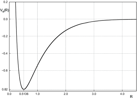
Fig. 1.: Symmetric electron term ($V_{s}(R)=U_{s}(R)+2.0+1/R$)

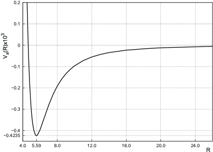
Fig. 2.: Antisymmetric electron term ($V_{a}(R)=U_{a}(R)+2.0\,+$ $+\,1/R$)

Table 1.: Parameters of symmetric
($s$) and antisymmetric ($a$) terms in 2$D$
and 3$D$ problems

$s$
	$R_{\min}$	$V_{\min}$	$R_{0}$	$R_{13}$
$2D$	0.51357	$-$0.820	0.2391	0.5821
$3D$	1.99719	$-$0.102635	1.10
$a$
	$R_{\min}$	$V_{\min}$	$R_{0}$	$R_{13}$
$2D$	5.59	$-4.235\times 10^{-4}$	4̇.625	3.9994
$3D$	12.55	$-6.08\times 10^{-5}$	10.69

The features in the solution of problem (14) in the BO adiabatic approximation are analogous to the difficulties faced with when solving the problem of three particles, irrespective of the difficulties in the numerical calculation of integrals (16); however, we will not discuss this issue.

The results of calculations carried out for the lowest terms (the ground states) in the symmetric and antisymmetric states, which were obtained for the 2$D$ problem, are depicted in Figs. 1 and 2, respectively.  The results of calculation for the symmetric term completely agree with the result of work [12] obtained in a different way.  Note that, in this formulation, the polar (spherical) symmetry is absent, and, from the general point of view, all states can be classed in the hyperspheroidal coordinates, where the total separation of variables can be executed (see works [12,​ 1,​ 2]).  For convenience, we presented terms (10) in such a form that they vanish as $R\rightarrow\infty$, which is convenient, while considering effective interaction potentials.  The value $U_{(s,a)}(\infty)=-2.0$ is the energy of one center (the hydrogen atom) in the ground state.  This is a two-particle decay threshold.  We would like to emphasize that the both terms $V_{(s,a)}(R)$ calculated for the lowest states in the 2$D$ problem remain negative (attraction) at significant distances ($R\gg 1$), as well as doubly degenerate in this limit (we consider the two-center problem), the same being also valid for the 3$D$ space.  At short distances (the two centers are united, $U_{(s)}(0)=-8,$ and $U_{(a)}(0)=-8/9$), the terms $V_{(s,a)}(R\rightarrow 0)$ are positive (repulsion) owing to the repulsive Coulomb potential between the identical centers.

The characteristic parameters of symmetric and antisymmetric 2$D$ terms (attractive potential wells) are quoted in Table 1, where a comparison with the corresponding parameters for the 3$D$ problem [4] is also made.  The Table demonstrates the positions of the minima, $R_{\mathrm{min}}$, the values of terms at the corresponding minima, $V_{\min}$, and the distance $R$, above which the terms are negative.  We would like to emphasize that the symmetric 2$D$ term is almost eight times as deep as the 3$D$ term (stronger coupling), and its position is located approximately four times nearer.  The distance $R_{0}$ in the 2$D$ case is also approximately four times shorter than that in the 3$D$ problem.  The minimum value of antisymmetric 2$D$ term is anomalously large in comparison with the 3$D$ term, but is much smaller than the value of symmetric term. This means that, similarly to the 3$D$ space, the conditions for the emergence of antisymmetric states are much poorer than the conditions, at which the symmetric states with the given charge, $Z$, and mass, $m$, values exist.  However, in the 2$D$ space, the antisymmetric term corresponds to a much stronger attraction than in the 3$D$ state.

Note that, in the BO approximation, the root-mean-square distance between the third (light) particle and one of the centers, $R_{31}$, which can be calculated using the electron functions $\Phi({\mathbf{r}},{\mathbf{R}}_{\mathrm{min}})$ according to the formula

$$R^{2}_{31}\equiv\langle R^{2}_{31}\rangle={\int d\mathbf{r}R^{2}_{31}\Phi^{2}(\mathbf{r},\mathbf{R}_{\min})}/{\int d\mathbf{r}\Phi^{2}(\mathbf{r},\mathbf{R}_{\min})}$$ (17)

satisfies the abnormal relation

$$R_{31}>R_{\mathrm{min}}$$ (18)

at the point $R_{\mathrm{min}}$ in the case of a symmetric main term. This relation was revealed in work [5], while carrying out three-particle calculations.  Hence, the fact is confirmed that the distance between the light particle and the attracting center calculated in the 2$D$ problem for large masses of two centers in molecular systems exceeds the distance between repulsive centers (let it be determined as $R_{\mathrm{min}}$).  However, the natural relation $R_{31}<R_{\mathrm{min}}$ takes place in the case of the 3$D$ problem.  In the 2$D$ problem, the natural relation is also obeyed for the antisymmetric state both in three-particle calculations [5] and in the BO approximation.

It is worth to note that, if considering the vibration states in the BO approximation, it is reasonable to consider only the terms indicated for the symmetric and antisymmetric ground states, because all other excited terms lie above the two-particle decay threshold $E_{0}(2)=-2.0$.  In Fig. 3, the main terms $s_{0}$ and $a_{0}$, as well as the excited symmetric term $s_{1}$ (designated as $U(R)$ for convenience), are shifted by the two-particle threshold energy, but are not shifted by the Coulomb potential, analogously to the 3$D$ problem.  The figure makes it evident that only the main terms can be responsible for the appearance of bound states in Eq. (9).

3 Term Asymptotics

Consider the asymptotics of 2$D$ terms at large and short distances, which are obtained according to the Schrödinger equation (8), and, if possible, let us make a generalization onto an arbitrary space dimensionality $d$.  This problem was already examined in a series of works by Lazur and coworkers [1,​ 2]. In this work, we will pay more attention to physical conclusions. The $d$-dimensional two-center Coulomb problem allows the separation of all variables in the hyperspheroidal coordinates; these are two linear coordinates, $\xi=(r_{1}+r_{2})/R$ and $\eta=(r_{1}-r_{2})/R$, and $d-2$ angular variables, in a full analogy with the 3$D$ space (see, e.g., works [4,​ 12]).  In the space of $\xi$ and $\eta$ coordinates, the problem for the lowest states that are independent of the angles is reduced to the following system of two coupled one-dimensional equations:

$$\begin{array}[]{l}\displaystyle(\xi^{2}-1)\dfrac{d^{2}X}{d\xi^{2}}+2\sigma\xi\dfrac{dX}{d\xi}\,+\\[8.53581pt] \displaystyle+\left(\dfrac{ER^{2}}{2}(\xi^{2}-1)+2R(\xi-1)+2R+RA\right)X=0,\\[8.53581pt] \displaystyle(1-\eta^{2})\dfrac{d^{2}Y}{d\eta^{2}}-2\sigma\eta\dfrac{dY}{d\eta}\,+\\[8.53581pt] \displaystyle+\left(\dfrac{ER^{2}}{2}(1-\eta^{2})-RA\right)Y=0,\end{array}\!\!\!\!\!\!\!\!\!\!\!\!\!\!\!\!\!\!\!\!\!\!$$ (19)

where $\xi\geq 1$, $-R<\eta<R$, $U(R)$ is the term, $A$ is the separation parameter, and $\sigma=(d-1)/2$ defines the space dimensionality.

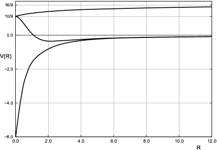
Fig. 3.: Ground ($s_{0},a$) and excited ($s_{1}$) electron terms

In all aspects, the system of one-dimensional equations (19) is similar to the known problem in the 3$D$ space.  Therefore, to derive an analytical solution, a standard perturbation theory can be developed for large and small distances $R$.  At large distances, where the symmetric and antisymmetric terms are degenerate to within an exponential accuracy, it is convenient to introduce the variables $\xi=1+\dfrac{2x}{R}$ ($x\geq 0$), and $\eta=1-\dfrac{2y}{R}$ ($0\leq y\leq R$) and, changing the variables,

$$X=\exp{\Bigg{\{}\!\!-\!\int\limits^{x}\!C(x^{\prime})dx^{\prime}\!\Bigg{\}}},\leavevmode\nobreak\ Y=\exp{\Bigg{\{}\!\!-\!\int\limits^{y}\!D(y^{\prime})dy^{\prime}\!\Bigg{\}}},$$ (20)

to consider the equations of the Riccati type,

$$\begin{array}[]{l}\displaystyle x\left(1+\dfrac{x}{R}\right)\left(-\dfrac{dC}{dx}+C^{2}\right)-\sigma\left(1+\dfrac{2x}{R}\right)\times\\[8.53581pt] \displaystyle\times\,C+2+A+2Ex\left(1+\dfrac{x}{R}\right)+\dfrac{4x}{R}=0,\\[8.53581pt] \displaystyle y\left(1-\dfrac{y}{R}\right)\left(-\dfrac{dD}{dy}+D^{2}\right)-\sigma\left(1-\dfrac{2y}{R}\right)\times\\[8.53581pt] \displaystyle\times\,D-A+2Ey\left(1-\dfrac{y}{R}\right)=0.\end{array}$$ (21)

We will use the so-called logarithmic perturbation theory in the small parameter $1/R$, when the energy, separation parameter, and solutions are sought in the form of a power series in the small parameter $1/R$ and satisfy equations of the Riccati type (see Eqs. (21)).  The final power series for the symmetric term of the ground state (as well as for the antisymmetric term, which is degenerate with the former in the power-law approximation) obtained from corresponding recurrent relations in the space of any dimensionality $d>1$ looks like

$$U_{0}(R)=-\frac{1}{2\sigma^{2}}-\frac{1}{R}-\frac{1}{R^{3}}\frac{1}{2}\sigma^{2}(1-\sigma^{2})\,-$$

$$-\,\frac{1}{R^{4}}\frac{1}{8}\sigma^{4}(1+\sigma)(5+4\sigma)-\frac{1}{R^{5}}\frac{3}{8}\sigma^{4}(1-\sigma^{2})(4-\sigma^{2})\,-$$

$$-\,\frac{1}{R^{6}}\frac{1}{4}\sigma^{6}(1+\sigma)(28+5\sigma-14\sigma^{2}-4\sigma^{3})+O\left(\!\frac{1}{R^{7}}\!\right)\!,$$ (22)

where four first terms reproduce the terms obtained in work [1].  The logarithmic derivatives of wave functions, obtained in the framework of perturbation theory, are

$$C(x,R)=\frac{1}{\sigma}+\frac{1}{R^{2}}\sigma\left(\!x+\frac{\sigma}{2}(1+\sigma)\!\right)-\frac{1}{R^{3}}\sigma x(x+\sigma)\,+$$

$$+\,\frac{1}{R^{4}}\sigma\biggl{[}x^{3}+x^{2}\frac{\sigma}{2}(3-2\sigma)-x\frac{\sigma^{2}}{4}\biggl{(}\!6\sigma^{2}\,+$$

$$+\,7\sigma-6\!\biggr{)}+\frac{3}{8}\sigma^{3}(1-\sigma^{2})(2+\sigma)\biggr{]}+O\left(\!\frac{1}{R^{5}}\!\right)\!,$$ (23)

$$D(x,R)=\frac{1}{\sigma}-\frac{1}{R^{2}}\sigma\left(\!y+\frac{\sigma}{2}(1+\sigma)\!\right)-\frac{1}{R^{3}}\sigma y(y+\sigma)\,-$$

$$-\,\frac{1}{R^{4}}\sigma\biggl{[}y^{3}+y^{2}\sigma\frac{3}{2}+y\frac{\sigma^{2}}{4}(6+\sigma)\,+$$

$$+\,\frac{3}{8}\sigma^{3}(1-\sigma^{2})(2+\sigma)\biggr{]}+O\left(\!\frac{1}{R^{5}}\!\right)\!.$$ (24)

However, the shift of the antisymmetric term with respect to the symmetric one has an exponential character irrespective of the space dimensionality,

$$\delta E=\frac{16}{\sigma^{3}\Gamma(\sigma)}\left(\!\frac{R}{2\sigma}\!\right)^{\!\!\sigma}e^{-R/\sigma-\sigma}\left[1+\frac{\sigma}{2R}+O\left(\!\frac{1}{R^{2}}\!\right)\!\right],$$ (25)

in accordance with the results of works [1,​ 4,​ 10] (here, $\Gamma(\sigma)$ is the gamma-function).

We would like to make a few general remarks.  First, the 2$D$ terms (10), taking into account Eq. (22), have an abnormal attractive asymptotics (22) of an order of $-1/R^{3}$.  Second, the asymptotic series (22) and, the more so, the power series near the exponent in Eq. (25) always diverge following the factorial law, which is well known to be a general rule for a diversity of problems in the 3$D$ space. Hence, such series can be used for estimations only at large enough distances.  Third, from the formal viewpoint, the computer facilities allow a significant number of higher power terms in series (22)–(25) to be calculated, but, generally speaking, this procedure has no reason because of the series divergence.  By the way, the character of divergence for such asymptotic series becomes weakened a little as the space dimensionality $d$ diminishes.  In particular, in the limit $d\rightarrow 1$, provided that $d$ is strictly larger than 1 and that this case has a physical sense, only the first terms in Eq. (22) would expectedly compose a good approximation for the term, even at moderate values of the distance $R$.

We would like to attract attention to one more important conclusion. In the 2$D$ space, the main asymptotics at large distances for the interaction potential of the van der Waals type between neutral atoms in ground states with zero angular momenta is the abnormal repulsion law $C/R^{5}$ rather than the standard attraction one $-A/R^{6}$ (in the 3$D$ space) even in the first order of perturbation theory.  In particular, in the 2$D$ space, as well as for an arbitrary dimensionality $d$, we have a repulsive potential of interaction of the quadrupole-quadrupole and quadrupole-dipole types between two hydrogen atoms at very large distances,

$$\dfrac{1}{R^{5}}\biggl{[}\dfrac{3}{4}\langle\hat{Q}_{2}(1)\rangle\langle\hat{Q}_{2}(2)\rangle+\dfrac{1}{2}\biggl{(}\!\!\langle\hat{d}(1)^{2}\rangle\langle\hat{Q}_{2}(2)\rangle\,+$$

$$+\,\langle\hat{d}(2)^{2}\rangle\ \langle\hat{Q}_{2}(1)\rangle\!\biggr{)}\!\biggr{]}=\dfrac{123}{1024}\dfrac{1}{R^{5}}.$$

Moreover, such abnormal repulsive asymptotics is of high importance in a space with a large enough dimensionality $d$, rather than in the 3$D$ one, where it vanishes, and in spaces with $d$ slightly exceeding 3, where a weak attractive asymptotics $-C/R^{5}$ is realized.  It should be recalled that, in this case, there also exists a centrifugal barrier of the kinematic origin, $(d-3)(d-1)/4R^{2}$.  The next asymptotic term, $-A/R^{6}$, which is obtained in the second-order perturbation theory in the dipole-dipole interaction parameter, is always attractive for an arbitrary space dimensionality.  Moreover, the constant $A$, most likely, can be much larger that the constant $C$ (in the term $-C/R^{5}$).  Therefore, the manifestation of the repulsive asymptotics in bound states can be strongly suppressed at a low dimensionality.  This conclusion is also supported by the presence of the centripetal attraction of the kinematic origin.

A separate attention should be attracted to the fact that the terms with the third, fifth, and some higher odd power exponents of the reciprocal radius in Eq. (22) are contributions of the first-order perturbation theory.  They are determined by the contributions of a quadrupole (the $1/R^{3}$-term in Eq. (22), it equals zero only in the 3$D$ space), octupole (the $1/R^{5}$-term), and sixth-order multipole (some part of the $1/R^{7}$-term) averaged over the wave function of one-center problem.  The $1/R^{4}$-term is a contribution of the second-order perturbation theory and describes the dipole-dipole interaction.  The $1/R^{6}$-term is a superposition of the dipole-octupole and quadrupole-quadrupole interactions in the second-order perturbation theory.  The remaining part of the $1/R^{7}$-term arises owing to the contribution of the dipole-quadrupole interaction in the third-order perturbation theory, and so on.  Really, the following expansion into a multipole series is valid at large distances $R$ between the centers:

$$\frac{1}{|\mathbf{r}-\mathbf{R}|}=\frac{1}{R}\sum\left(\!\frac{r}{R}\!\right)^{\!k}P_{k}\left(\!\frac{(\mathbf{r}\mathbf{R})}{rR}\!\right)=$$

$$=\frac{1}{R}\left(\!1+\frac{\hat{d}}{R}+\frac{\hat{Q}_{2}}{2R^{2}}+\sum\frac{\hat{Q}_{k}}{R^{k}}\!\right)\!,$$ (26)

where $P_{k}$ are the Legendre polynomials depending on the angle cosine $\cos(\phi)=({\mathbf{r}}{\mathbf{R}})/|{\mathbf{r}}||{\mathbf{R}}|$, $\hat{d}=z=r\cos(\phi)$ is the dipole moment operator, $\hat{Q}_{2}=(3z^{2}-r^{2})$ is the quadrupole moment operator, and $\hat{Q}_{k}=r^{k}P_{k}(\cos(\phi))$ are the operators of higher-order multipole moments.  Then the even multipole moments averaged over the spherically symmetric wave function of the ground state in the $d$-dimensional space,

$$\psi_{0}(r)=Be^{-r/\sigma},$$ (27)

must be, generally speaking, different from zero. The quadrupole moment equals (see work [5])

$$\left\langle\hat{Q}_{2}\right\rangle=\left\langle(3z^{2}-r^{2})\right\rangle=\dfrac{(3-d)(1+d)(d-1)^{2}}{16}.$$ (28)

Hence, it is positive (the system is elongated along the $z$-axis) in the 2$D$ space (as well as in the range $1<d<3$).  At $d>3$, it is negative (the system is flattened along the $z$-axis) and grows by absolute value according to the law $d^{4}$.  It is of interest that the quadrupole and all multipole moments tend to zero if the space dimensionality tends to 1, which is a consequence of the collapse.  The next, octupole, moment depending on the dimensionality $d$ looks like

$$\langle\hat{Q}_{4}\rangle=\left\langle\!\frac{1}{8}(35z^{4}-30z^{2}r^{2}+3r^{4})\!\right\rangle=$$

$$=\frac{3(d-1)^{4}(1+d)(9-d^{2})(5-d)}{2048}.$$ (29)

It equals zero in the 3$D$ and 5$D$ spaces and remains positive for $1<d<3$ and negative for $3<d<5$ (as all even multipole moments do). At $d>5$, the octupole moment $\left\langle Q_{4}\right\rangle$ is positive again.  The general formula for nonzero even multipole moments in the ground state reads

$$\langle\hat{Q}_{2n}\rangle=\frac{(2n-1)!!}{2^{5n}n!}(d-1)^{2n}(d+1)(3^{2}-d^{2})\,\times$$

$$\times\,(5^{2}-d^{2})(7^{2}-d^{2})\mbox{...}\left((2n-1)^{2}-d^{2}\right)(2n+1-d).$$ (30)

A consequence of the general formula (30) consists in that the multipole moments $\left\langle\hat{Q}_{2n}\right\rangle$ in the spaces with odd dimensionalities equal zero if $d\leq 2n+1$ and oscillate $n$ times if $d>2n+1$; for even dimensionalities ($d=2n$), they always differ from zero.  Therefore, all multipole moments averaged over the spherically symmetric wave functions vanish only in the 3$D$ space (and, formally, in the 1$D$ space as a result of the collapse), but it is not so for even dimensionalities and other odd and fractal ones.  In the 5$D$ space, all multipoles equal zero in a spherically symmetric field, except for the quadrupole, which is negative in this case.  In the 7$D$ space, all multipoles equal zero, but for the quadrupole, which is negative, and the octupole, which is positive, and so on.  Note also that the averaging of the multipole expansion (26) gives rise to a factorially divergent asymptotic series, and the character of divergence grows with the space dimensionality $d$.

Similar regularities are also observed for average multipole moments in excited states.  For instance, for the first radially excited state, the Coulomb wave function is

$$\Psi_{1}(r)=B\left\{\!1-\dfrac{r}{\sigma(\sigma+1)}\!\right\}\exp\left\{\!-\dfrac{r}{\sigma+1}\!\right\}\!.$$ (31)

The angular part remains the same as for the ground state.  Therefore, the quadrupole moment is equal to

$$\left\langle 1|\hat{Q}_{2}|1\right\rangle=\frac{(d+1)^{2}(d+11)(3-d)}{16},$$ (32)

and the octupole moment to

$$\left\langle 1|\hat{Q}_{4}|1\right\rangle=\frac{3(d+1)^{4}(d+29)(3^{2}-d^{2})(5-d)}{128}$$ (33)

with all general regularities being similar to those in the ground state.  Let us consider a state with the angular moment equal 1 (the $P$ state).  In this case, the wave function of the one-center problem is

$$\Psi_{P}(r)=Bz\exp\left\{-\dfrac{r}{\sigma+1}\right\},$$ (34)

the energy equals $E_{1}=-2/(d+1)^{2},$ and the quadrupole moment

$$\left\langle P|\hat{Q}_{2}|P\right\rangle=\frac{(d+1)^{2}(d+3)(7-d)}{16}$$ (35)

evidently differs from zero in the 3$D$ geometry. The octupole,

$$\langle P|\hat{Q}_{4}|P\rangle=\frac{3(d+1)^{4}(d+5)(3^{2}-d^{2})(21-d)}{2048},$$ (36)

and higher multipole moments also oscillate and vanish for the increasing number of odd $d$-values.  For even $d$-values, all multipoles are nonzero again.

Making allowance for the dipole interaction $z/R^{2}$ (the second term in Eq. (26)) in the framework of perturbation theory for the 2$D$ space and at any $d$ (in high-order terms of the small parameter $1/R^{2}$) deserves a special attention. In those cases, we obtain a multidimensional Stark problem for a hydrogen atom in a uniform electric field,

$$\left\{\!-\frac{1}{2}\Delta-\frac{1}{r}+\epsilon z\!\right\}\Psi=E\Psi,$$ (37)

with $\epsilon\equiv 1/R^{2}$.  Let us consider the energy shift for the ground state, when only the contributions of terms with even power exponents of $\epsilon$ survive: the Stark effects of the second, fourth, and so on, orders.  Note that the quadratic Stark effect was already contained in formula (22) as the fourth term.  Analogously to the 3$D$ case (see work [12]), the hyperparabolic coordinates allow the separation of variables in Eq. (37) to be done, so that, for the angle-independent ground state, we obtain the system of 1$D$ equations

$$\begin{array}[]{l}\displaystyle\left(\!\xi\dfrac{d^{2}}{d\xi^{2}}+\sigma\dfrac{d}{d\xi}+\dfrac{E}{2}\xi-\dfrac{\epsilon}{4}\xi^{2}+\beta_{1}\!\right)\chi(\xi)=0,\\[8.53581pt] \displaystyle\left(\!\eta\dfrac{d^{2}}{d\eta^{2}}+\sigma\dfrac{d}{d\eta}+\dfrac{E}{2}\eta+\dfrac{\epsilon}{4}\eta^{2}+\beta_{2}\!\right)\phi(\eta)=0,\\[8.53581pt] \displaystyle\beta_{1}+\beta_{2}=1,\end{array}$$ (38)

which is identical formally to the equations for the 3$D$ Stark effect, provided the substitution $1\rightarrow\sigma=$ $=(d-1)/2$ in terms before the first derivative.  After the change of variables,

$$\chi=\exp{\Bigg{\{}\!\!-\!\int\limits^{\xi}\!F(\xi^{\prime})d\xi^{\prime}\!\Bigg{\}}},\quad\displaystyle\phi=\exp{\Bigg{\{}\!\!-\!\int\limits^{\eta}\!G(\eta^{\prime})d\eta^{\prime}\!\Bigg{\}}}$$ (39)

the linear second-order equations for the ground state are reduced to a system of two nonlinear first-order equations of the Riccati type,

$$\begin{array}[]{l}\displaystyle-\dfrac{dF}{d\xi}+F^{2}-\dfrac{\sigma}{\xi}F+\dfrac{E}{2}-\dfrac{\epsilon}{4}\xi+\frac{\beta_{1}}{\xi}=0,\\[8.53581pt] \displaystyle-\dfrac{dG}{d\eta}+G^{2}-\dfrac{\sigma}{\eta}G+\dfrac{E}{2}+\dfrac{\epsilon}{4}\eta+\frac{\beta_{2}}{\eta}=0,\\[8.53581pt] \displaystyle\beta_{1}+\beta_{2}=1.\end{array}$$ (40)

The system of equations (40) is rather convenient for the application of perturbation theory (the logarithmic perturbation theory in the form of recurrent relations), if its solutions are sought in the form of power series in the small parameter $\epsilon$,

$$\begin{array}[]{l}\displaystyle F(\epsilon,\zeta)=\sum\limits_{n}\epsilon^{n}F_{n}(\zeta),\\[14.22636pt] \displaystyle G(\epsilon,\eta)=\sum\limits_{n}\epsilon^{n}G_{n}(\eta),\end{array}$$ (41)

with the coefficient functions taken in the form of polynomials.  Then, taking only the dipole interaction into account, we obtain the nonzero contributions to the energy in the even orders of perturbation theory (the generalized Stark law),

$$E_{0}=-\frac{1}{2}\sigma^{2}-\frac{1}{R^{4}}\frac{\sigma^{4}}{8}(1+\sigma)(5+4\sigma)-\frac{1}{R^{8}}\sigma^{10}(1+\sigma)\,\times$$

$$\times\,(192\sigma^{3}+933\sigma^{2}+1550\sigma+880)+O\left(\!\frac{1}{R^{12}}\!\right)\!.$$ (42)

The second term in Eq. (42) coincides with the fourth one in formula (22).  Note that series (42) in the small parameter $1/R^{4}$ also diverges factorially at the fixed $\sigma=(d-1)/2$.

In view of the results obtained above for multipoles in the asymptotic expressions for term (22), we note that the available asymptotics $1/R^{3}$ (the polarizability of the first order according to perturbation theory) has a quadrupole origin and is negative (attraction) for $1<d<3$ (in particular, for the 2$D$ problem) and positive (repulsion) for $d>3$.  Moreover, the higher the space dimensionality, the stronger is the repulsion in the $1/R^{3}$-asymptotics.  The term of the second order in the dipole-dipole interaction (the polarizability of the second order) for the ground state always corresponds to the attraction (the negative term).

At short distances, where the problem of finding the asymptotics becomes even more complicated (see work [2]), the terms have the following behavior: for the symmetric ground state,

$$U_{s}(R)=-8+64R^{2}\ln\left(\!\frac{1}{2}e^{C}R\!\right)+O(R^{2}),$$ (43)

where $C=0.57722...$ is the Euler constant, for the lowest state of the antisymmetric term,

$$U_{a}(R)=-\frac{8}{9}-\frac{80}{9}R^{2}+O(R^{4}),$$ (44)

and, for the first excited symmetric term,

$$U_{s}(R)=-\frac{8}{9}+\frac{64}{27}R^{2}\ln\left(\!\frac{3}{2}e^{C+1}R\!\right)+O(R^{2}).$$ (45)

4 Approximation Formulas for Terms

For the application of energy terms to be convenient, we will derive the approximation formulas for the symmetric and antisymmetric ground terms $V_{s,a}(R)$ in the 2$D$ space.  The approximations account for the results of direct calculations shown in Figs. 1 and 2, as well as the asymptotic behavior of the terms at short and large distances discussed in the previous section.

For the symmetric term in the short-distance interval ($R<0.1$), we use the asymptotics [1,​ 2] $V_{s}(R)=1/R-6+64R^{2}\ln(1/2e^{C}R)$.  At large distances ($R>6.5$), we use asymptotics (22) and (25), when we may put

$$V_{s}(R)=-\frac{3}{32}\frac{1}{R^{3}}-\frac{21}{256}\frac{1}{R^{4}}-\frac{135}{2048}\frac{1}{R^{5}}\,-$$

$$-\,\frac{159}{1024}\frac{1}{R^{6}}-\frac{32}{\pi e}e^{-2R}\left(\!1+O\left(\!\frac{1}{R}\!\right)\!\right)\!.$$ (46)

In the intermediate region, we use approximation formulas in the form of the ratio between polynomials of the distance $R$,

$$V_{s,{\rm appr}}(R)\!=\!\dfrac{b_{0}\!+\!b_{1}R\!+\!b_{2}R^{2}+\!\mbox{...}\!+\!b_{n-2}R^{n-2}}{R(a_{0}\!+\!a_{1}R\!+\!a_{2}R^{2}\!+\!\mbox{...}\!+\!a_{n}R^{n})}.$$ (47)

which should involve two first asymptotic terms at short distances and all known power-law asymptotics at large ones.  The account of the power-law asymptotics at large and short distances, as well as the linearity in the sought parameters in the numerator and the denominator, imposes the following additional relations:

$$\begin{array}[]{l}\displaystyle b_{0}=a_{0},\\ \displaystyle b_{1}=a_{1}-6a_{0},\\ \displaystyle b_{2}=a_{2}-6a_{1},\\ \displaystyle b_{3}=1{,}0,\\ \displaystyle b_{n-2}=-(3/32)a_{n},\\ \displaystyle b_{n-3}=-(3/32)a_{n-1}-(21/256)a_{n},\\ \displaystyle b_{n-4}=-(3/32)a_{n-2}\!-\!(21/256)a_{n-1}\!-\!(135/2048)a_{n},\\ \displaystyle b_{n-5}=-(3/32)a_{n-3}-(21/256)a_{n-2}\,-\\ \displaystyle-\,(135/2048)a_{n-1}-(159/1024)a_{n}.\end{array}\!\!\!\!\!\!\!\!\!\!\!\!\!\!\!\!\!\!\!\!\!\!$$ (48)

The parameters $a_{k}$ and $b_{i}$ were determined using the procedure of best fitting to the calculated term in the range $0.1<R<6.5$ according to the $\chi_{\mathrm{and}}^{2}$-criterion; the corresponding $\chi_{\mathrm{and}}^{2}=1.2\times 10^{-6}$. To obtain a satisfactory approximation in Eq. (47), it was enough to take $n=9$ and to neglect the last abnormal term in Eq. (46).  In this case, the parameters to fit were only 10 quantities $a_{k}$ in the denominator of Eq. (46).  Their values are listed in Table 2.  All parameters in the numerator of Eq. (46) were unambiguously determined from relations (48).

Table 2.: Approximation coefficients
for symmetric and antisymmetric terms

$i$	$a_{i},s$	$a_{i},a$	$b_{i},a$
0	0.13241	1.5067
1	1.84394	0.9674
2	4.12047	1.3044
3	1.30497	0.073
4	1.29747	2.5425	$-2{.}1696$
5	0.03477	0.8491	0.4898
6	$-0{.}00581$	$-0{.}3083$
7	0.19956	$-3{.}4974$
8	$-0{.}06119$	3.0725	1.8518
9	0.01156	0.072605

An approximation formula similar to Eq. (47) was used for the antisymmetric term:

$$V_{a,{\rm appr}}(R)=\{b_{0}+b_{1}R+b_{2}R^{2}+\mbox{...}+b_{n-2}R^{n-2}+$$

$$+b_{n-1}\;32R^{n+1}\exp(-2R-1)/\pi\}/$$

$$/\{R(a_{0}+a_{1}R+a_{2}R^{2}+\ldots+a_{n}R^{n})\}.$$ (49)

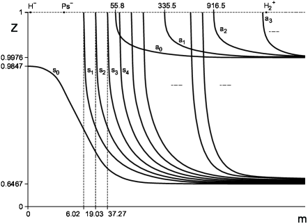
Fig. 4.: Diagrams (schematically) of the energy level stability for a two-dimensional system of three charged particles

Table 3.: Critical mass values
$m_{\mathrm{crit}.}^{(n)}$ for symmetric states with (the second row) and without (the third row) regard for the abnormal centripetal attraction $-\frac{1}{4r^{2}}$

State $n$	0	1	2	3	4	5
Total potential	0	6.01	19.03	37.27	59.03	84.43
without $-(1/4)/r^{2}$	0.75	8.09	22.19	42.67	68.92	99.89
3-part. calc.	0	5.9	20.2	40.9	67.2	98.3

Table 4.: Critical mass values $m_{\mathrm{crit}.}^{(n)}$
for antisymmetric states with (the second row)
and without (the third row) regard for the abnormal
centripetal attraction $-\frac{1}{4r^{2}}$

State $n$	0	1	2	3	4
Total potential	55.8	335.5	916.5	1741.5	2807
without $-(1/4)/r^{2}$	128.3	509.2	1155.5	2063.5	3229
3-part. calc.	111	643	1675	3266	5690

The difference consists in that the abnormal asymptotics (the last term with the opposite sign) from Eq. (46) is taken now into account, and we have the short-distance asymptotics $V_{a}(R)=1/R+10/9+O(R^{2})$.  This means that, in the second and third formulas of Eqs. (48), the coefficient $-6$ should be better substituted by $10/9$.  In addition, we neglect the last two relations from Eqs. (48) in the numerator of Eq. (49).  The other parameters in the numerator of Eq. (49) are unambiguously determined by relations (48).  The obtained values of approximation parameters (at $n=9$) for the antisymmetric term are quoted in Table 2 (the third and fourth columns).  We hope for that the accuracy of the approximations obtained for both symmetric and antisymmetric terms is high enough for those terms to be used in further researches.

It is worth noting that the symmetric term in the 2$D$ problem decreases according to the asymptotic law $-1/R^{3}$ in the preasymptotic region of large distances.  As a result, there is no reason for the realization of the preasymptotic law $-1/R^{2}$, which was discussed in work [13] for neutral atoms in the 3$D$ case.

5 Stability Diagrams
in the Born-Oppenheimer
Adiabatic Approximation

The determined terms allow us, in accordance with Eq. (9), to find vibration spectra in the BO approximation and to plot the corresponding stability diagrams (for the three-particle problem in the 2$D$ space, they were found in work [5]).  In Fig. 4, the curves of stability threshold calculated for the symmetric $(s_{n})$ and antisymmetric $(a_{n})$ states in the BO adiabatic approximation are exhibited schematically.  The corresponding curves on the plane $(m,Z)$ mean that the $n$-th symmetric state exists to the right from the corresponding curve $s_{n}$, whereas the $n$-th antisymmetric state exists to the right from the corresponding curve $a_{n}$.  Certainly, although the diagrams are plotted for all values of mass ratio $m$, one should bear in mind that the BO adiabatic approximation is physically justified only for the molecular mode, so that the results obtained for small $m$-values are shown only to make a more complete comparison with the results of direct three-particle calculations taken from work [5]. Tables 3 and 4 also demonstrate the results of calculation, according to simple Eq. (9), of critical masses $m_{\mathrm{crit}.}^{(n)}$ for the symmetric and antisymmetric states, when $Z=1$ and the energy $\varepsilon=0$. Those values are partially shown in Fig. 4: they determine vertical asymptotes.  We also calculated the simple 1$D$ problem (9) with the effective potentials $V_{\mathrm{eff}}(r)=V(r)-(1/4/(m+1/2))/r^{2}$ both in the full variant (the second rows in Tables 3 and 4) and neglecting the second term associated with the kinetic energy of the centripetal attraction (Eq. (9)) (the third rows in Tables 3 and 4). The last rows show the results of three-particle calculations for the critical values $m_{\mathrm{crit}.}^{(n)}$ (more accurate in comparison with work [5] and carried out using a Gaussian basis with 1300 components).

Let us compare various variants of critical mass, $m_{\mathrm{crit}.}$, sets in more details.  First of all, we should pay attention to that the BO adiabatic approximation is a variational estimate “from above” for the energies and critical values $m_{\mathrm{crit}.}^{(n)}$. Therefore, all the curves in Fig. 4 calculated in the BO approximation must lie above those calculated in the three-particle problem and be more correct if the mass $m$ is larger.  From a comparison of the second and fourth rows in Table 3, it follows that, while calculating the symmetric state in the framework of the three-particle scheme, the accuracy higher than that attained in the BO approximation was obtained only for the first two states.  Hence, the calculation of the terms and the vibration level energies in the adiabatic approximation turns out justified from the viewpoint of accuracy and the understanding of regularities.  To a larger extent, those remarks concern anomalously weakly coupled antisymmetric states. From a comparison of the second and fourth rows in Table 3, it follows that even the substantially corrected, in comparison with work [5], results of calculations (using the basis of about 1100 Gaussoid-like components) turn out unsatisfactory at the quantitative level in comparison with the results obtained in the BO approximation.  At last, a comparison of the results in the second (the total effective term) and third (here, the centripetal attraction $-(1/4)/r^{2}$ is neglected) rows of Tables 3 and 4 allows us to evaluate the order of the contribution given by this centripetal attraction to the stability diagram structure.  For instance, neglecting the centripetal attraction in the symmetric ground state always gives rise to a finite critical mass, whereas, for higher excitations, the difference between the results in the second and third rows becomes larger and larger.  A special attention should be paid to the fact that, in the 2$D$ problem and in the adiabatic approximation for the ground state, we obtain a bound three-particle level at any mass value, which follows from the known fact [15,​ 16] that, in the case of two particles and an attractive potential, there always exists at least one weakly bound state with the energy that exponentially depends on the potential, $E_{0}=-(\hbar^{2}/mr_{0}^{2})\exp(\mathrm{Const}/v_{0}+C2)$, where $v_{0}$ is the zero-momentum Fourier component of the attractive potential, $v_{0}<0$.

Concerning the horizontal asymptotes in Fig. 4, the threshold curves determine the minimum value of charge

$$Z_{\mathrm{crit}}=\min\left\{[1-RV_{s}(R)]^{-1}\right\},$$ (50)

for symmetric and antisymmetric states in the limit of large mass $m$.  For the corresponding $R_{\mathrm{crit}(s)}=0.89$ in the symmetric state, we obtain $Z_{\mathrm{crit}(s)}=0.64686$, and this value coincides with the results of three-particle calculations [5].  Accordingly, the antisymmetric threshold curves have the minimum $Z_{\mathrm{crit}(a)}=$ $=0.9976$, and $R_{\mathrm{crit}(a)}=5.7$.  The indicated values were determined more exactly than it could be done in three-particle calculations.

Note also that the results of three-particle calculations according to Eq. (14) imply that there are no antisymmetric bound states for all masses at dimensionalities $d>3.337$.  This is a result of the repulsion provided by both the centrifugal barrier $l_{\mathrm{eff}}(l_{\mathrm{eff}}+1)/R^{2}$, where $l_{\mathrm{eff}}=(d-3)/2$ is the effective angular hypermomentum, and the repulsive asymptotics $\left\langle Q_{2}\right\rangle/2R^{3}$ of term (22) with the abnormal quadrupole moment of a hydrogen atom.  In this case, as the dimensionality grows, the antisymmetric term becomes exclusively repulsive (it remains attractive only in the 2$D$ and 3$D$ problems, if the space dimensionality is an integer number).  In turn, the results of three-particle calculations according to Eq. (14) demonstrate that symmetric states are absent for all masses $m$ only at large space dimensionalities, when $d>9$, and the bound state of an atomic hydrogen ion is absent at $d>6$.  This follows from the presence of the centrifugal barrier $(d-3)(d-1)/4R^{2}$, abnormal quadrupole moment, and repulsion $\left\langle Q_{2}\right\rangle/2R^{3}$.

Note at last that the results of calculations for the critical masses $m_{\mathrm{crit}(s)}$ of various states in the BO approximation can be approximated by a square law, depending on the number of a state (in the case of 3$D$ problem, this was done in work [5]).  In particular, for the symmetric states,

$$m_{\mathrm{crit}(s),n}=2.47(n+1)^{2}-3.3.$$ (51)

This formula is much more exact than the approximation obtained from three-particle calculations [5], especially for high excited states. The general constant at $n^{2}$ in Eq. (51) is determined as the asymptotics of the quasiclassical approximation

$$m_{\mathrm{crit}}=(\pi/J)^{2}n(n+1),$$ (52)

in which the quasiclassical integral (neglecting the centripetal attraction)

$$J=1.84785$$

and, accordingly,

$$\left(\!\frac{\pi}{J}\!\right)^{\!2}=2.89$$

are determined only by the negative part of the term. Similarly, for the antisymmetric critical states, we obtain the approximation

$$m_{\mathrm{crit}(s),n}=138.6n(n+1)+51,$$ (53)

and, from the quasiclassical approximation for antisymmetric states,

$$\left(\!\frac{\pi}{J}\!\right)^{\!2}=129.845.$$

Note that the quasiclassical estimation for the asymptotics of energy levels in the 2$D$ case is not well-grounded.  There are principal difficulties in the estimation of quasiclassical integrals at both large and short distances owing to the centripetal attraction $-1/(4R^{2})$.

As a consequence of those approximations, it follows from the adiabatic approximation that there are 26 excited levels for a molecular hydrogen ion H${}_{2}^{+}$ (with the mass $m=1836.152701)$ in the symmetric state.  In the antisymmetric state, the total number of levels equals four.

6 Final Remarks

To summarize, we would like to note that the researches carried out for three charged particles in the framework of Born–Oppenheimer approximation allowed us to establish a number of abnormal regularities arising in the 2$D$ space and the spaces of arbitrary dimensionality.  In the 2$D$ space, the multipole expansions for Coulomb potentials in a spherically symmetric field are nonzero. Also nonzero are the quadrupole, octupole, and other multipole moments in the $d$-dimensional problems.  In the 2$D$ problem, the quadrupole moment of a hydrogen atom is positive and generates an attractive asymptotics $\sim$$-1/R^{3}$ for the ground-state term, whereas, in the 3$D$ problem, this contribution equals zero.  As a result, it was found that a hydrogen atom in the 2$D$ space is polarizable already in the first-order perturbation theory. Expressions for higher multipole moments in spaces with arbitrary dimensionalities are obtained and analyzed.  The antisymmetric terms of trions $XXY$ are attractive only in the 2$D$ and 3$D$ problems.  Moreover, it is shown that there is a critical dimensionality value $d_{\mathrm{crit}}=3.337$, and there are no bound antisymmetric states in spaces with $d>d_{\mathrm{crit}}$.  The abnormal behavior of the asymptotics for interaction potentials of the van der Waals type between neutral hydrogen atoms in the 2$D$ space is demonstrated.

The convenient approximation formulas for 2$D$ terms are proposed.  In the framework of the Born–Oppenheimer adiabatic approximation, the stability diagrams for the 2$D$ space are obtained, and the main characteristic asymptotics for the stability threshold curves for trions $XXY$ are plotted and analyzed.  They agree with the stability diagrams obtained earlier in three-particle calculations.

The authors express their gratitude to M.V. Kuzmenko​, who participated in this research atthe initial stage, and to B.E. Grynyuk for the useful discussion of effective numerical calculation proce-dures.

I.В. Сименог, В.В. Михнюк, Ю.М. Бiдасюк
ЕНЕРГЕТИЧНI ТЕРМИ ТА ДIАГРАМИ
СТАБIЛЬНОСТI ДЛЯ 2$D$ ЗАДАЧI
ТРЬОХ ЗАРЯДЖЕНИХ ЧАСТИНОК
Р е з ю м е
Для двовимiрних кулонiвських систем типу симетричних трiонiв $XXY$ у варiацiйному пiдходi отримано симетричний та антисиметричний терми. Дано якiсне пояснення дiаграм стабiльностi та певних аномалiй в $2D$ просторi на основi адiабатичного наближення Борна–Опенгаймера. Виконано аналiз отриманих для довiльної вимiрностi простору асимптотик енергетичних термiв на великих вiдстанях, i запропоновано апроксимацiйнi формули для $2D$ термiв. Встановлено аномальну залежнiсть мультипольних моментiв вiд вимiрностi простору у випадку сферично-симетричного поля. Проведено кiлькiсне порiвняння основних результатiв для $2D$ i $3D$ задач двох кулонiвських центрiв.

References

- [1] D.I. Bondar, V.Yu. Lazur, I.M. Shvab, and S. Halupka, Zh. Fiz. Dosl. 9, 304 (2005).
- [2] D.I. Bondar, M. Gnatich, and V.Yu. Lazur, Teor. Mat. Fiz. 148, 269 (2006).
- [3] T.K. Rebane and A.V. Filinskii, Yad. Fiz. 60, 1985 (1997).
- [4] I.V. Simenog, Yu.M. Bidasyuk, M.V. Kuzmenko, and V.M.Hryapa, Ukr. Fiz. Zh. 54, 881 (2009).
- [5] I.V. Simenog, V.V. Mikhnyuk, and M.V. Kuzmenko, Ukr. Fiz. Zh. 58, 290 (2013).
- [6] M.A. Lampert, Phys. Rev. Lett. 1, 450 (1958).
- [7] K. Kheng et al., Phys. Rev. Lett. 71, 1752 (1993).
- [8] I.V. Komarov, L.I. Ponomarev, and S.Yu. Slavyanov, Spheroidal and Coulomb Spheroidal Functions (Nauka, Moscow, 1976) (in Russian).
- [9] L.V. Keldysh, Pis’ma Zh. Eksp. Teor. Fiz. 20, 716 (1979).
- [10] Y. Suzuki and K. Varga, Stochastic Variational Approach to Quantum-Mechanical Few-Body Problems (Springer, Berlin, 1998).
- [11] P. Duclos, P. Stovicek, and M. Tusek, J. Phys. A 43, 474020 (2010).
- [12] L.D. Landau and E.M. Lifshitz, Quantum Mechanics. Non-Relativistic Theory (Pergamon Press, New York, 1977).
- [13] D. Yiwu, Z. Guanghui, B. Chengguang et al., Sci. China A 39, 317 (1996).
- [14] D.A. Kirzhnits and F.M. Pen’kov, Zh. Èksp. Teor. Fiz. 85, 80 (1983).
- [15] L.V. Bruch and J.A. Tjon, Phys. Rev. A 19, 425 (1979).
-
[16]
I.V. Simenog, preprint ITP-80-12E (Institute for Theoretical
Physics, Kiev, 1980).
Received 28.10.13.
Translated from Ukrainian by O.I. Voitenko