Relativistic positioning: errors due to uncertainties in the satellite world lines

Abstract

Global navigation satellite systems use appropriate satellite constellations to get the coordinates of an user –close to Earth– in an almost inertial reference system. We have simulated both GPS and GALILEO constellations. Uncertainties in the satellite world lines lead to dominant positioning errors. In this paper, a detailed analysis of these errors is developed inside a great region surrounding Earth. This analysis is performed in the framework of the so-called relativistic positioning systems. Our study is based on the Jacobian ($J$) of the transformation giving the emission coordinates in terms of the inertial ones. Around points of vanishing $J$, positioning errors are too large. We show that, for any 4-tuple of satellites, the points with $J=0$ are located at distances, D, from the Earth centre greater than about $2R/3$, where $R$ is the radius of the satellite orbits which are assumed to be circumferences. Our results strongly suggest that, for D-distances greater than $2R/3$ and smaller than $10^{5}\ km$, a rather good positioning may be achieved by using appropriate satellite 4-tuples without $J=0$ points located in the user vicinity. The way to find these 4-tuples is discussed for arbitrary users with $D<10^{5}\ km$ and, then, preliminary considerations about satellite navigation at $D<10^{5}\ km$ are presented. Future work on the subject of space navigation –based on appropriate simulations– is in progress.

Keywords relativistic positioning systems; methods: numerical; reference systems

1 Introduction

It is often stated that, at distances –from Earth– greater than $D_{max}\sim 2\times 10^{4}\ km$, positioning errors are too big and, consequently, satellite navigation based on global navigation satellite systems (GNSS) is not feasible (see Deng et al. (2013) and references cited therein). This topic about spacecraft navigation is revisited in this paper, where the formalism of the so-called relativistic positioning systems (RPS) is used. In any RPS, the location of an user (spacecraft, car on Earth, and so on) may be achieved by receiving appropriate data from four satellites of a certain GNSS (only GPS and GALILEO constellations are here considered)

Hereafter, index $A$ labels the four satellites, any other Latin index runs from $1$ to $3$, and Greek indexes from $1$ to $4$. Quantities $G$, $M_{\oplus}$, $t$, and $\tau$ stand for the gravitation constant, the Earth mass, the coordinate time, and the proper time, respectively. Quantities $\eta_{\alpha\beta}$ are the covariant components of the Minkowski metric tensor, lengths are given in kilometres and the time unit is defined in such a way that the speed of light is $c=1$.

User location requires the choice of a certain reference system. It is usually an almost inertial reference. The satellite world lines must be known in this reference. Uncertainties in these lines lead to positioning errors. The analysis of this type of errors is the main goal of this paper.

In any RPS, the user receives codified signals from four satellites at the same time. After decoding, these signals provide the user with the satellite proper times at emission. These four proper times are the so-called emission coordinates $\tau^{A}$ of the observation event. From these proper times, the user coordinates in the almost inertial reference (hereafter inertial coordinates $x^{\alpha}$) must be calculated; namely, the user position must be found. Sometimes there are two possible user positions (bifurcation). See Schmidt (1972); Abel & Chaffee (1991); Chaffee & Abel (1994); Grafarend & Shan (1996). In this case, additional information is necessary to get the true position (Coll, Ferrando & Morales-Lladosa, 2011, 2012; Puchades & Sáez, 2012).

For photons moving in Minkowski space-time, the user inertial coordinates, $x^{\alpha}$, and the emission ones, $\tau^{A}$, must satisfy the following algebraic equations:

$$\eta_{\alpha\beta}[x^{\alpha}-x^{\alpha}_{A}(\tau^{A})][x^{\beta}-x^{\beta}_{A}(\tau^{A})]=0\ ,$$ (1)

where $\eta_{\alpha\beta}$ is a diagonal matrix with $\eta_{11}=\eta_{22}=\eta_{33}=1$ and $\eta_{44}=-1$, and the points of the satellite world lines have inertial coordinates $x^{\beta}_{A}(\tau^{A})$, which must be well known functions of the proper times $\tau^{A}$. According to Eqs. (1), photons follow null geodesics from satellite emission to user reception. These algebraic equations may be solved by using both the satellite world lines and the numerical Newton-Raphson method (Press et al., 1999).

Eqs. (1) may be numerically solved for the unknowns $\tau^{A}$ by assuming that the position coordinates $x^{\alpha}$ are known. Thus, the emission coordinates are obtained from the inertial ones. However, the same equations may be solved to get the unknowns $x^{\alpha}$ for known emission coordinates $\tau^{A}$. This second case gives the inertial coordinates in terms of the emission ones (positioning); nevertheless, this second numerical solution of Eqs. (1) is not necessary since there is an analytical formula obtained by Coll, Ferrando & Morales-Lladosa (2010), which gives $x^{\alpha}$ in terms of $\tau^{A}$ for photons moving in Minkowski space-time, and arbitrary satellite world lines.

We use a manageable approach which leads to an accurate enough positioning. In this approach, the satellite world lines are appropriate timelike geodesics of the Schwarzschild space-time, and the photons follow null geodesics in the Minkowski space-time asymptotic to the Schwarzschild geometry.

In our approach, there are two types of positioning errors. The first one is due to the fact that photons do not move in Minkowski space-time, but in the Earth gravitational field. In the simplest generalization of the above approach, it may be assumed that both satellites and photons move in the Schwarzschild space-time created by an ideal spherically symmetric Earth. Space-time metrics more general than the Minkowski one have been considered in previous papers (Bahder 2001; Čadež & Kostić 2005; Bini et al. 2008; Ruggiero & Tartaglia 2008; Teyssandier & Le Poncin-Lafitte 2008; Delva & Oplympio 2009; Čadež, Kostić & Delva 2010; Bunandar, Caveny & Matzner 2011; Delva, Kostić & Čadež 2011). Metrics including Earth rotation and deviations with respect to the spherical symmetry in the Earth mass distribution might be also considered; nevertheless, since the distance travelled by the photons from the satellites to any possible user is not large, and the Earth gravitational field is weak, the lensing effect produced by this field –on the photons– is expected to be small and, consequently, positioning errors of the first type should be small. A detailed study about these errors will be presented elsewhere. This paper is devoted to study a second type of positioning errors, which are due to uncertainties in the satellite world lines. These errors are greater than those due to our assumption that photons move in Minkowski space-time (first type). The equations of the satellite world lines are involved in Eqs. (1) and, consequently, any uncertainty in the satellite motions leads to positioning errors when Eqs. (1) are solved (either analytically or numerically) to find the user position from the emission coordinates.

Any GNSS is based on a certain satellite constellation whose world lines (orbits and motions) have been appropriately designed. Their equations are known in the almost inertial system of reference. Hereafter, we say that these satellites form the ideal constellation. Of course, these ideal world lines are not followed by the true satellites. Even if they are launched to follow them, gravity, radiation pressure, and so on, would produce deviations with respect to the ideal lines. Sometimes these deviations are too large and the satellite world lines must be corrected. In this way, the space and time deviations of the true world lines with respect to the ideal ones would keep smaller than a certain upper limit (deviation amplitude), which is hereafter assumed to be $10^{-2}\ km$ and $10^{-2}$ time units, respectively.

We simulate the world lines of the GALILEO and GPS background configurations. The GPS constellation has $n_{s}=24$ satellites which move in six different orbital planes (four satellites per plane), each plane inclined an angle $\alpha_{in}=55\ deg$ with respect to the equator. To obtain around two orbits per day, the satellites are placed at an altitude $h=20200\ km$. We have numerated the satellites in such a way that the satellites 1 to 4, 5 to 8, 9 to 12, 13 to 16, 17 to 20, and 21 to 24 correspond to different consecutive orbital planes. The GALILEO constellation is composed by 27 satellites ($n_{s}=27$), located in three equally spaced orbital planes (9 uniformly distributed satellites in each plane). The inclination of these planes is $\alpha_{in}=56\ deg$ and the altitude of the circular orbits is $h=23222\ km$; thus, the orbital period is close to 14.2h. The satellites are numerated as in the GPS case; namely, satellites 1 to 9, 10 to 18, and 19 to 27 are placed in distinct consecutive orbital planes. All the trajectories are assumed to be circumferences whose centres are located in the Earth centre, which is also the origin of the almost inertial reference system used for positioning.

In order to take into account the effect of the Earth gravitational field on the satellite clocks, which run more rapid than clocks at rest on Earth (about 38.4 microseconds per day for GPS), it is assumed that satellites move in Schwarzschild space-time, where the circumferences are possible satellite trajectories, which are followed with angular velocity $\Omega=(GM_{\oplus}/R^{3})^{1/2}$. In the asymptotically almost inertial system associated to the Schwarzschild space-time created by Earth, up to first order in the small parameter $GM_{\oplus}/R$, the coordinates of a given satellite $A$ may be written as follows:

$$x^{1}_{A} = R\,[\cos\alpha_{A}(\tau)\cos\psi+\sin\alpha_{A}(\tau)\sin\psi\cos\theta]$$

$$x^{2}_{A} = -R\,[\cos\alpha_{A}(\tau)\sin\psi-\sin\alpha_{A}(\tau)\cos\psi\cos\theta]$$

$$x^{3}_{A} = -R\sin\alpha_{A}(\tau)\sin\theta$$

$$x^{4}_{A} = \gamma\tau\ ,$$ (2)

where factor $\gamma$ is given by the relation (Ashby, 2003)

$$\gamma=\frac{dt}{d\tau}=1+\frac{3GM_{\oplus}}{2R}\ ,$$ (3)

and the angle

$$\alpha_{A}(\tau)=\alpha_{A0}-\Omega\gamma\tau$$ (4)

localizes the satellite on its trajectory. For any satellite, angles $\theta$ and $\psi$ and $\alpha_{A0}$ are constant. The two first angles define an orbital plane in a certain GNSS, whereas the third angle fixes the position of satellite $A$ at $\tau=x^{4}=0$. See Puchades & Sáez (2012) for more details.

A numerical code with multiple precision has been designed to calculate the emission coordinates $\tau^{A}$ (unknowns) from the inertial ones (data) by solving Eqs. (1). It is hereafter referred to as the XT-code. This code –based on the Newton-Raphson numerical method– requires the satellite world line equations; that is to say, there must be a subroutine which calculates the inertial coordinates of every satellite $x^{\alpha}_{A}$ for any value of $\tau^{A}$. For the ideal world lines, this calculation is done by using Eqs. (2)–(4), but the subroutine may work with any known perturbation of these lines (see below). Other world lines allowed by the Schwarzschild geometry, e.g., motions along almost elliptical orbits, could be also implemented in the subroutine; however, it is not done in this paper since our main results about positioning errors would keep unaltered.

The paper is organized as follows, in Sect. 2, an analytical formula giving the user coordinates in terms of the emission ones, which was derived by Coll, Ferrando & Morales-Lladosa (2010) in Minkowski space-time is briefly described. Positioning errors due to uncertainties in the satellite world lines are studied in Sect. 3. Sect. 3.1 is a theoretical discussion about these errors, whereas Sect. 3.2 contains numerical calculations and results. Finally, a general discussion and some comments about perspectives are presented in Sect. 4.

2 Analytical formula for the positioning transformation $x^{\alpha}=x^{\alpha}(\tau^{A})$

In this section we use the same compact notation as in Coll, Ferrando & Morales-Lladosa (2010). The inertial coordinates of any event are denoted $x\equiv(x^{1},x^{2},x^{3},x^{4})\equiv(\vec{x},t)$.

The coordinates ($x^{1},x^{2},x^{3},x^{4}$) of the satellite $A$, at emission time $\tau^{A}$, are denoted $\gamma_{A}$. Since the world lines of the satellites are known, quantities $\gamma_{A}$ may be calculated for arbitrary proper times. The three vectors $e_{a}=\gamma_{a}-\gamma_{4}$ define the relative positions between satellites $A=a$ and $A=4$. The numeration of the satellites and, consequently, the choice of the fourth satellite are arbitrary. We may say that vectors $e_{a}$ define the internal satellite configuration at emission times. There are inertial coordinates characterizing an user who receives the times $\tau^{A}$ from the satellites, if and only if, the so-called emission-reception conditions, Coll, Ferrando & Morales-Lladosa (2010), are satisfied. These conditions may be written as follows:

$$\eta_{\alpha\beta}e_{a}^{\alpha}e_{a}^{\beta}>0,\,\,\,\,\eta_{\alpha\beta}(e_{a}^{\alpha}-e_{b}^{\alpha})(e_{a}^{\beta}-e_{b}^{\beta})>0\ ,$$ (5)

for any value of indexes $a$ and $b$.

The general transformation from emission to inertial coordinates was derived in Coll, Ferrando & Morales-Lladosa (2010); it is a solution of Eqs. (1), which is valid for arbitrary satellite world lines. In compact formalism, this solution may be written as follows:

$$x=\gamma_{4}+y_{\ast}-\frac{y_{\ast}^{2}\chi}{(y_{\ast}\cdot\chi)+\hat{\epsilon}\sqrt{(y_{\ast}\cdot\chi)^{2}-y_{\ast}^{2}\chi^{2}}}\ ,$$ (6)

where vectors $\chi$ and $y_{\ast}$ may be calculated from $e_{1}$, $e_{2}$, and $e_{3}$ (internal satellite configuration). The configuration vector $\chi=\ast(e_{1}\wedge e_{2}\wedge e_{3})$ (dual of a double exterior product) is orthogonal to the hyperplane containing the four $\gamma_{A}$ emission events. Vector $y_{\ast}=(\xi,H)/(\xi\cdot\chi)$, where $(\xi,H)$ stands for the interior product, may be calculated from any arbitrary vector $\xi$ satisfying the condition $\xi\cdot\chi\neq 0$ and from the bivector $H=[(e_{a}\cdot e_{a})/2]E^{a}$, where $E^{1}=\ast(e_{2}\wedge e_{3})$, $E^{2}=\ast(e_{3}\wedge e_{1})$, and $E^{3}=\ast(e_{1}\wedge e_{2})$. Finally, quantity $\hat{\epsilon}$ (orientation of the emission coordinates at $x$) can only take on the values $+1$ and $-1$.

In practice, our numerical codes have been designed by using tensor components in the almost inertial system of reference; this procedure requires a change of notation. From the compact notation used in Eq. (6) –which is very appropriate for many purposes– we have passed to index notation (tensor components). The basic formulae necessary to do this change were explicitly given in a recent paper by Coll, Ferrando & Morales-Lladosa (2012). By using index notation, we have built up a numerical code –based on Eq. (6)– which, for given emission coordinates $\tau^{A}$, allows us the calculation of the user inertial coordinates $x^{\alpha}$. This code is hereafter referred to as the TX-code. Of course, as in the case of the XT-code described above, a subroutine calculating the inertial coordinates of every satellite at given values of $\tau^{A}$ is necessary. This subroutine has the same structure in both codes since it has been designed to find points of the satellite world lines.

Since the transformation defined by Eq. (6) is the solution of Eqs. (1) for the unknowns $x^{\alpha}$, and Eqs. (1) express that the distance from $\gamma_{A}$ to $x$ vanishes (in Minkowski space-time), two types of solutions may be obtained. The first type corresponds to signals emitted from the satellites at times $\tau^{A}$ and received by an user, at the same time $t$, at position $\vec{x}$ (emission or past-like solutions). The second type describes a signal emitted from position $\vec{x}$ at time $t$ and received by the satellites at times $\tau^{A}$ (reception or future-like solutions). Only the first type is significant for positioning.

In Coll, Ferrando & Morales-Lladosa (2010), it was proved that, for $\chi^{2}\neq 0$, there are two sets of inertial coordinates corresponding to $\hat{\epsilon}=+1$ and $\hat{\epsilon}=-1$. Moreover, for $\chi^{2}<0$, only one of the two sets of inertial coordinates corresponds to a positioning solution. In the case $\chi^{2}>0$, the number of positioning solutions may be either two or zero, in the first case, there are two different receptors (located at different places), which would receive the same four emission times from the same satellites. In the second case, there are two future-like solutions. Finally, for $\chi^{2}=0$ there is only a single positioning solution.

Given four proper times $\tau^{A}$ compatible with conditions (5), our TX-code calculates all the positioning (past-like) solutions of Eqs. (1).

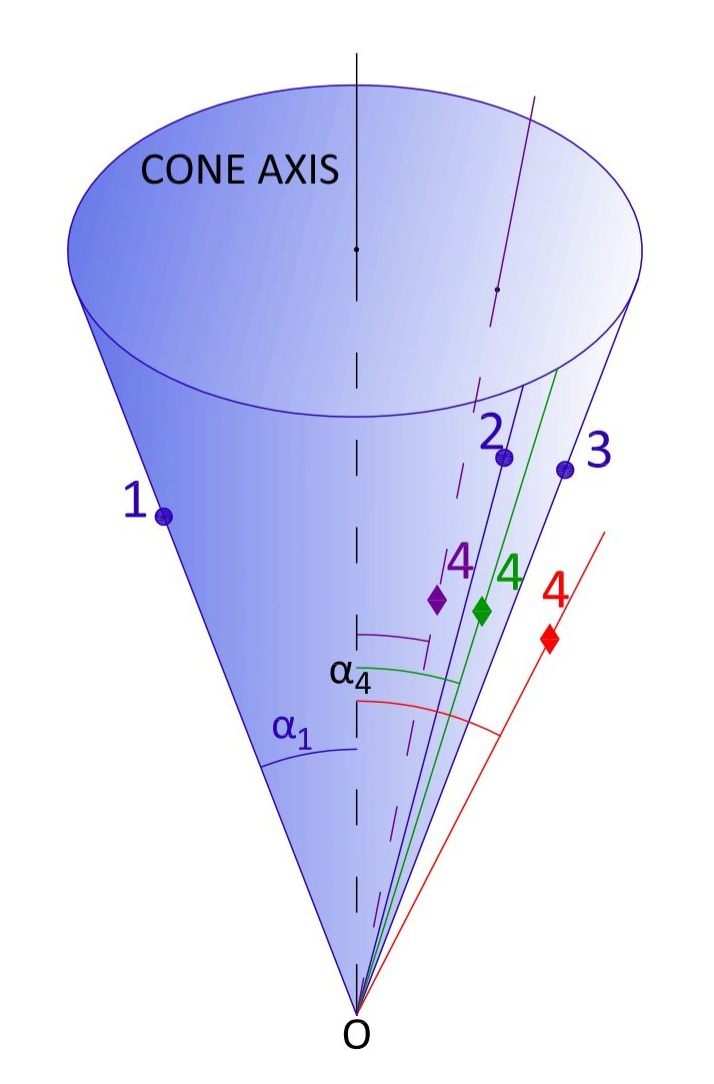
Fig. 1 : User-satellites configurations and Jacobian values: the cone is generated by the user $O$ and the three satellites 1, 2, and 3. For the green position of satellite 4, the four satellites are in the surface of the same cone with vertex at $O$, where $J$ vanishes. Satellite 4 is not on the cone surface for the red and fuchsia positions, for which $J$ does not vanish at $O$.

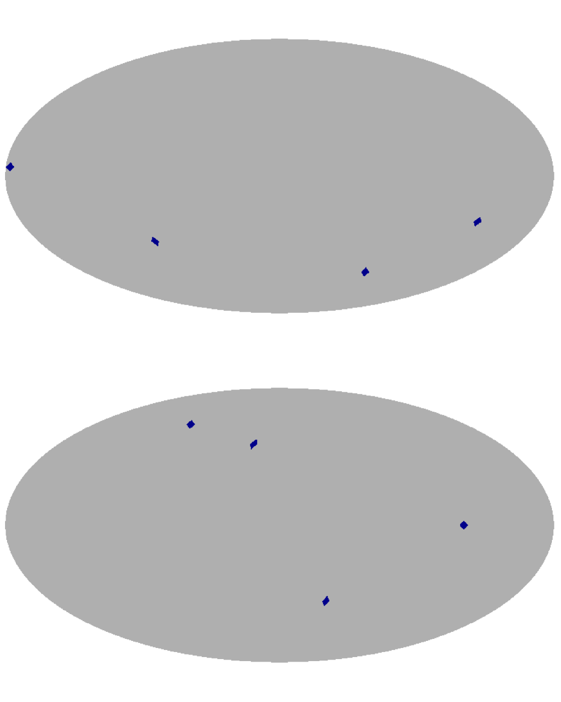
Fig. 2 : GALILEO satellites 2, 5, 20, and 23 are observed –from point $E$– in the blue pixels at inertial times $t=19\ hours$ (top) and $t=25\ hours$ (bottom)

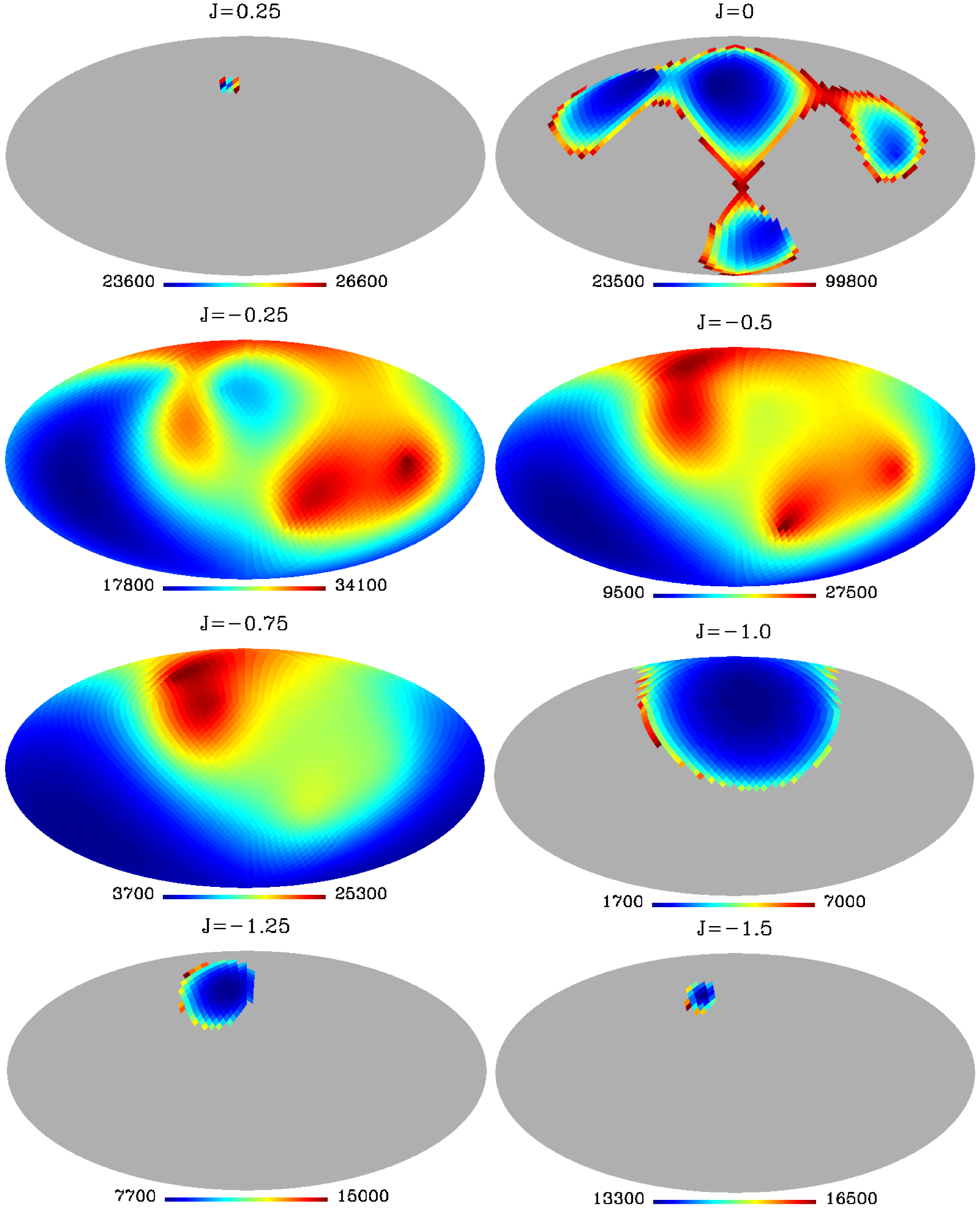
Fig. 3 : HEALPIx mollwide maps for the bottom configuration of Fig. 1. The quantity represented is the distance, $L_{1}$, from $E$ to the closest point where the Jacobian $J$ takes on the fixed value displayed above the map

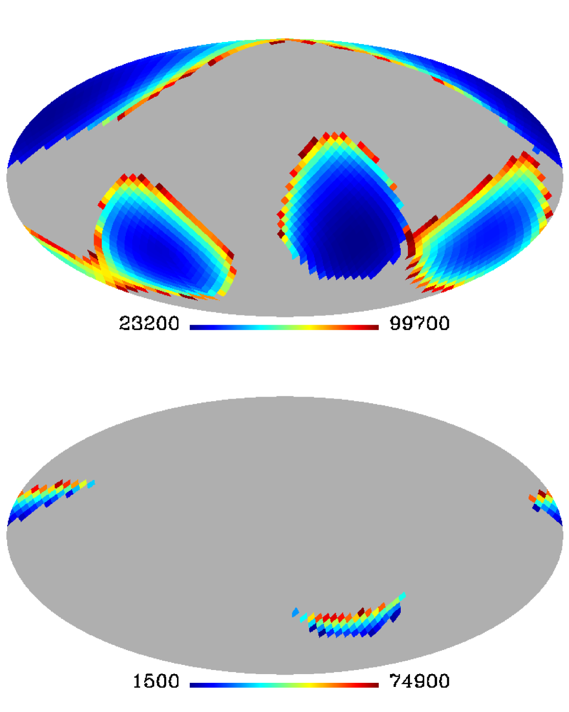
Fig. 4 : Top: Same representation as in Fig. 3 for the top configuration of Fig. 2 and $J=0$. Bottom: HEALPIx mollwide map of the distance, $L_{12}$, from the first to the second point where $J=0$ (same configuration as in the top panel).

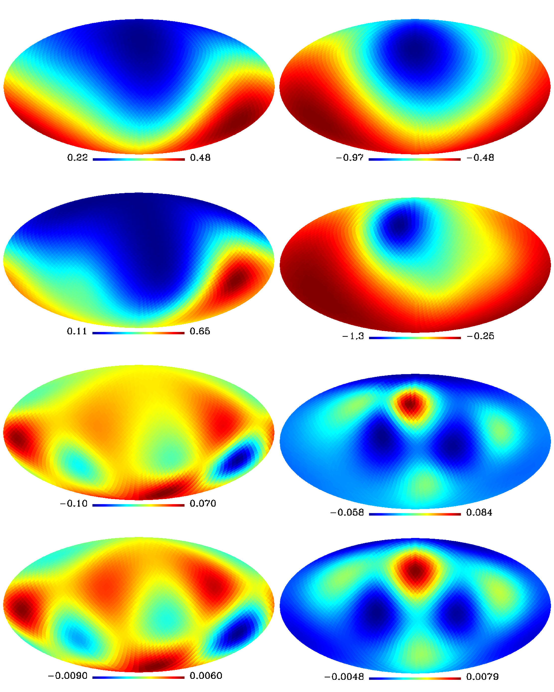
Fig. 5 : Left (right): HEALPIx mollwide maps of the $J$ values on spheres with different radius for the top (bottom) configuration of Fig. 2. From top to bottom, the radius of the spheres in kilometres are $6378=R_{\oplus}$, $1.5\times 10^{4}$, $5\times 10^{4}$ and $9\times 10^{4}$.

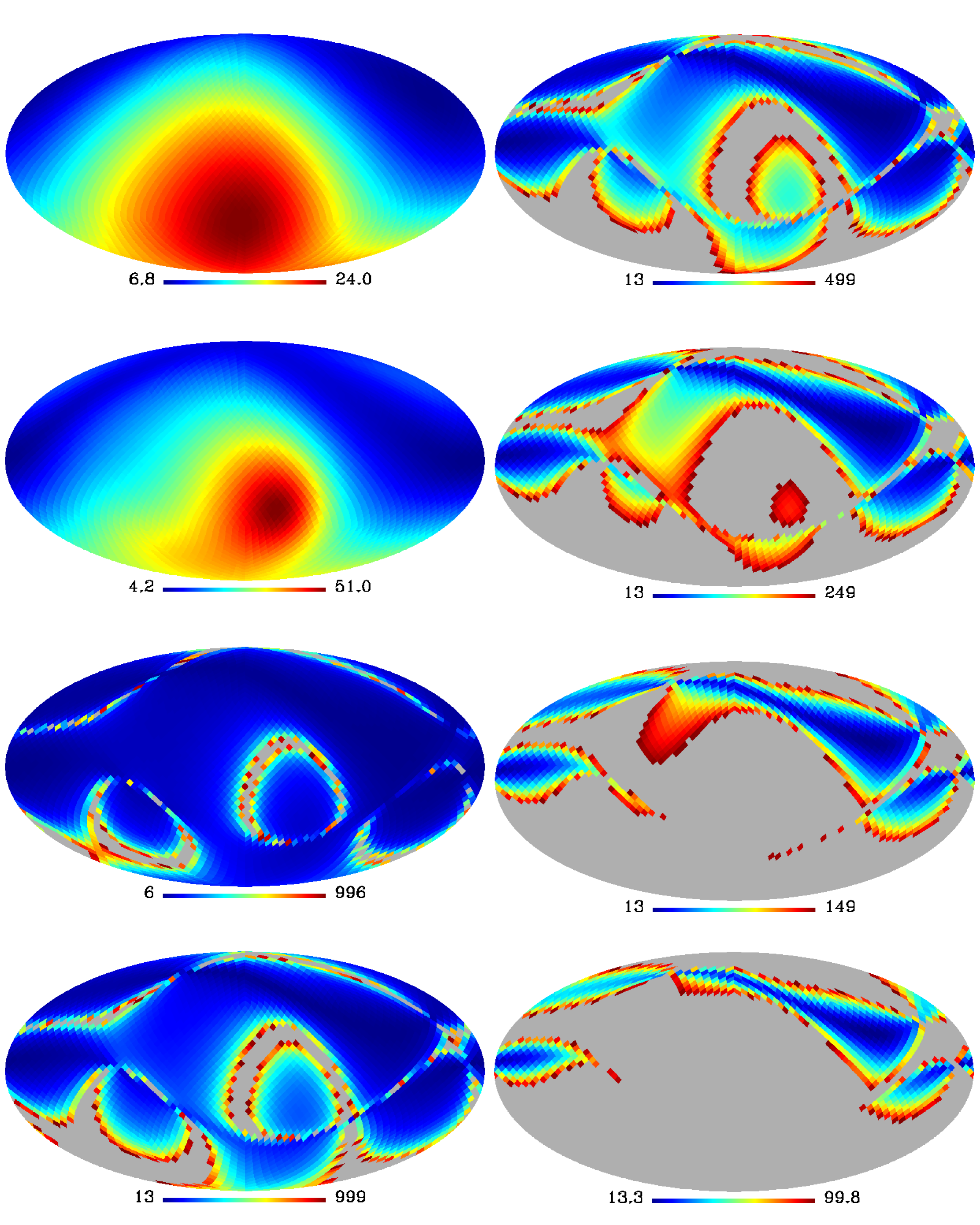
Fig. 6 : Left: HEALPIx mollwide maps of $\Delta_{d}$ values, in meters, for the same spheres and configuration as in the left panels of Fig. 5. Gray (colored) pixels in the middle-bottom and bottom panels are characterized by the condition $\Delta_{d}\geq 10^{3}\ m$ ($\Delta_{d}<10^{3}\ m$). The scale separating gray and colored pixels is $10^{3}\ m$. Right: same sphere and configuration as in the left bottom panel. From top to bottom, the scales, in meters, separating gray from colored pixels are $500$, $250$, $150$ and $100$

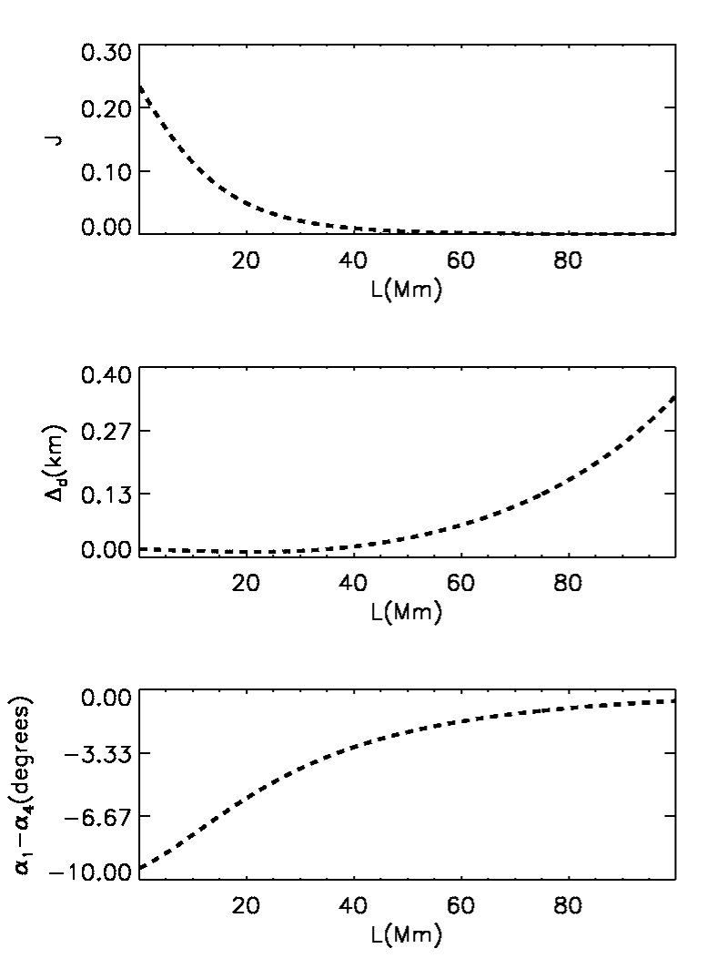
Fig. 7 : The values of $J$ (top), $\Delta_{d}$ (middle) and $\alpha_{1}-\alpha_{4}(bottom)$ are represented along a certain direction from $L=0$ (point $E$) to $L=10^{2}\ Mm$. The chosen segment, where $J$ does not vanish, corresponds to the top configuration of Fig. 2.

Fig. 8 : Same quantities and configuration as in Fig. 7, for a direction where $J$ vanishes once. In this Figure, the two middle panels are $\Delta_{d}$ representations. The middle-top panel includes all the large $\Delta_{d}$ values obtained close to the point of vanishing $J$. In the middle-bottom panel, all the $\Delta_{d}$ values greater than $100\ m$ have been eliminated to make visible the positioning errors far from the $J=0$ point.

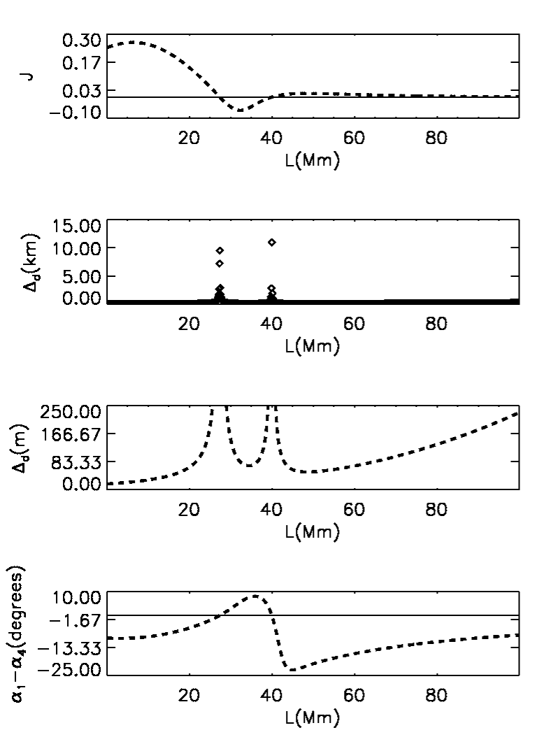
Fig. 9 : Same representation as in Fig. 8 for a direction where $J$ vanishes twice

3 Positioning errors due to uncertainties in the satellite world lines

Positioning errors have been studied in various papers (Langley 1999, Puchades & Sáez 2011; Sáez & Puchades 2013, 2014). In Langley (1999), GPS positioning errors due to the receiver-satellites geometry were studied. It was claimed that these errors strongly depend on the volume of the tetrahedron formed by the tips of the four user-satellites unit vectors. The larger the volume, the smaller the positioning errors. In Sec 3.1, the tetrahedron criterion is justified in the framework of relativistic positioning. Preliminary work in the line of the present paper was presented in some workshops (Puchades & Sáez, 2011; Sáez & Puchades, 2013, 2014). Here, a more general relativistic four dimensional (4D) study is presented, this study is extended far from Earth to see the size of the region where positioning is accurate enough. Outside this region, either pulsar navigation methods or other suitable techniques (Deng et al., 2013) might be useful.

3.1 Theoretical considerations

With the essential aim of analyzing positioning errors, let us assume that: (i) users are located inside a sphere centred at point $E$, whose radius is $10^{5}\ km$. It is hereafter referred to as the $E$-sphere. The centre $E$ is fully arbitrary. For a given user with coordinates $x^{\alpha}$, positioning results do not depend on the chosen $E$. The spherical inertial coordinates of $E$ have been chosen to be $r_{E}=R_{\oplus}$, $\theta_{E}=60^{\circ}$, and $\phi_{E}=30^{\circ}$, where $R_{\oplus}$ is the Earth radius. Hence, point E is on the Earth surface, (ii) all the users have the same inertial time coordinate; namely, they belong to the hypersurface $x^{4}=constant$. This constant time is arbitrary, but it must be a few seconds greater than the initial time, $t_{in}$, of the GNSS operation; thus, the signals emitted by the satellites may be received by the users, and (iii) opaque objects –as Earth– intercepting the signal broadcast by the satellites are not taken into account, these objects may be easily considered after, without modifying our main conclusions about positioning errors.

Under the simplifying condition (iii), any user with inertial coordinates $x^{\alpha}$, satisfying conditions (i) and (ii), simultaneously receives codified signals –with the emission proper times $\tau^{A}$– from any set of four satellites of the ideal GNSS constellation. Moreover, any neighbouring user would receive very similar proper times from the same satellites. These facts strongly suggest that, in some open set containing the point $P$ with coordinates $x^{\alpha}$, there is a function $\tau^{A}=\tau^{A}(x^{\alpha})$ which is continuous and has continuous partial derivatives, in other words, it is a $C^{1}$ function. Then, according to the inverse function theorem, there is a $C^{1}$ function $x^{\alpha}=x^{\alpha}(\tau^{A})$ in some open set containing $Q$ (image of P), if and only if, the Jacobian $J=|\partial\tau^{A}/\partial x^{\alpha}|$ is a non vanishing real number at $P$. Evidently, any user receiving emission coordinates close to those of point $Q$ (from the four chosen satellites) should be close to the user at $P$. This condition requires a $C^{1}$ inverse function $x^{\alpha}=x^{\alpha}(\tau^{A})$ with continuous partial derivatives at $Q$ and, consequently, the Jacobian $J$ must be different from zero at $P$. A vanishing $J$ at point $P$ suggests strong positioning problems around this point. Large positioning errors are expected –in the region surrounding $P$– for any consistent definition of these errors. This expectation has been numerically verified (see below).

The Jacobian of the inverse function $x^{\alpha}=x^{\alpha}(\tau^{A})$ is $J^{\prime}=1/J=|\partial x^{\alpha}/\partial\tau^{A}|$. If this Jacobian is a non vanishing real number at $Q$, $J$ is also a non vanishing real number at $P$ and positioning is possible

In order to calculate the partial derivatives involved in $J$, we may use Eqs. (1) with well defined satellite world lines. From these four equations, one easily finds the following formula

$$\frac{\partial\tau^{A}}{\partial x^{\alpha}}=\frac{\zeta[x^{\alpha}-x^{\alpha}_{A}(\tau^{A})]}{\eta_{\mu\nu}U^{\mu}_{A}(\tau^{A})[x^{\nu}-x^{\nu}_{A}(\tau^{A})]}\ ,$$ (7)

where $\zeta=1$ for $\alpha=1,2,3$ and $\zeta=-1$ for $\alpha=4$. The inertial coordinates $x^{\alpha}_{A}(\tau^{A})$ and the four-velocity $U^{\mu}_{A}(\tau^{A})=dx^{\mu}_{A}/d\tau^{A}$ of satellite $A$ may be easily calculated, at any given proper time $\tau^{A}$, by means of Eqs. (2)–(4). Hence, given an user with inertial coordinates $x^{\alpha}$, our XT-code gives the corresponding emission coordinates $\tau^{A}$ and, then, the partial derivatives involved in $J$ may be calculated by using Eqs. (7) and Eqs. (2)–(4).

The satellite four velocity may be calculated with the formula $U^{\mu}_{A}(\tau^{A})=\gamma^{A}(v^{1}_{A},v^{2}_{A},v^{3}_{A},1)$, where $v^{i}_{A}$ are the components of the satellite velocity in the almost inertial reference, and $\gamma^{A}=[1-(v_{A})^{2}]^{-1/2}$ is the Lorentz factor of satellite $A$. Since the satellite speeds are much smaller than unity, $U^{\mu}_{A}(\tau^{A})$ may be approximated by the four-vector (0,0,0,1) for any $A$. Hence, the following relation is approximately satisfied: $\eta_{\mu\nu}U^{\mu}_{A}(\tau^{A})[x^{\nu}-x^{\nu}_{A}(\tau^{A})]\simeq x^{4}_{A}(\tau^{A})-x^{4}=-D_{A}$, where $D_{A}$ is the distance from the user to the position of satellite $A$ at emission time. On account of this relation, Eqs. (7) may be rewritten as follows:

$$\frac{\partial\tau^{A}}{\partial x^{\alpha}}\simeq\frac{\zeta[x^{\alpha}_{A}(\tau^{A})-x^{\alpha}]}{D_{A}}$$ (8)

and, consequently, the Jacobian is the value of the following determinant

$$\,\,\,\,\,\,\left|\begin{array}[]{cccc}\frac{1}{D_{1}}(x^{1}_{1}-x^{1})&\frac{1}{D_{1}}(x^{2}_{1}-x^{2})&\frac{1}{D_{1}}(x^{3}_{1}-x^{3})&1\\ &&&\\ \frac{1}{D_{2}}(x^{1}_{2}-x^{1})&\frac{1}{D_{2}}(x^{2}_{2}-x^{2})&\frac{1}{D_{2}}(x^{3}_{2}-x^{3})&1\\ &&&\\ \frac{1}{D_{3}}(x^{1}_{3}-x^{1})&\frac{1}{D_{3}}(x^{2}_{3}-x^{2})&\frac{1}{D_{3}}(x^{3}_{3}-x^{3})&1\\ &&&\\ \frac{1}{D_{4}}(x^{1}_{4}-x^{1})&\frac{1}{D_{4}}(x^{2}_{4}-x^{2})&\frac{1}{D_{4}}(x^{3}_{4}-x^{3})&1\\ \end{array}\right|$$

Let us now calculate the volume of the tetrahedron formed by the tips of the four user-satellites unit vectors. Since the system is not relativistic (small velocities), the volume may be calculated in any inertial reference system (almost invariance under Lorentz transformations). If the coordinate origin is chosen to be the user position, the coordinates of the tetrahedron vertexes are $\frac{1}{D_{A}}(x^{\alpha}_{A}-x^{\alpha})$ and, consequently, the absolute value of the above $4\times 4$ determinant is exactly six times the tetrahedron volume $V_{T}$; namely, the relation $V_{T}=|J|/6$ is satisfied. Therefore, it has been proved that, due to the small satellite speeds, $|J|$ is well approximated by $6V_{T}$. This fact justifies the study carried out by Langley (1999) in the framework of GPS, in which, $V_{T}$ appears to be correlated with positioning errors (dilution of precision).

The partial derivatives $\partial x^{\alpha}/\partial\tau^{A}$ involved in the Jacobian $J^{\prime}$ may be also directly computed from Eqs. (1), but it is not necessary since $J^{\prime}$ may be calculated by using the derivatives given by Eq. (7) and the relation $J^{\prime}=1/J$.

As it was proved by Pozo & Coll (2006) and Coll, Ferrando & Morales-Lladosa (2012), the Jacobian $J$ vanishes if and only if the four satellites are on the same cone surface with the user in the vertex. This is valid for any satellite configuration, even for a relativistic one with very high velocities. In the sketch of Fig. 1, configurations with $J=0$ and $J\neq 0$ may be distinguished. The user located at vertex $O$ and the satellites 1, 2, and 3 (at emission times) generate a cone. Quantities $\alpha_{1}$ and $\alpha_{4}$ are the angles between the cone axis and the lines of sight of satellite 1 and 4, respectively. Hence, the Jacobian $J$ vanishes at $O$ if and only if $\alpha_{1}-\alpha_{4}=0$ (green position), whereas it is different from zero for the red (fuchsia) position of satellite 4, in which, this satellite is not on the cone surface but outside (inside).

It is evident that, for standard low velocity satellite systems and $\alpha_{1}=\alpha_{4}$, the tips of the four user-satellites unit vectors are on the same plane orthogonal to the cone axis and, consequently, the relation $V_{T}=0$ is satisfied. Moreover, if the user is very far from the satellites, they are all in a small solid angle and the tetrahedron volume $V_{T}$ is expected to be small. Our numerical estimates are in agreement with these considerations, since we have found that, close to the points $x^{\alpha}$ where $J$ vanishes and $J^{\prime}$ diverges, small uncertainties in the satellite world lines lead to large positioning errors, and we have also verified that, for users $x^{\alpha}$ located far enough from the satellites, the Jacobian $J$ is small and, accordingly, the positioning errors are big.

Let us first suppose that the satellites move, without uncertainties, according to Eqs. (2)–(4). These equations describe the satellite world lines in the case of a spherically symmetric non rotating Earth, in the absence of external actions. In practice, any realistic satellite world line deviates with respect to the ideal ones given by Eqs. (2)–(4). If the ideal world lines are parametrized by means of their proper times, the equations of these lines may be written as follows: $y^{\alpha}=x^{\alpha}_{A}(\tau^{A})$. Then, the realistic perturbed world lines may be written in the following form $y^{\alpha}=x^{\alpha}_{A}(\tau^{A})+\xi^{\alpha}_{A}(\tau^{A})$ in terms of the same parameters. Functions $\xi^{\alpha}_{A}(\tau^{A})$ measure the deviations between realistic and ideal world lines. These deviations are unavoidable.

The ideal world lines of the satellites are those of Sect. 1. The trajectories are circumferences travelled as it corresponds to the Schwarzschild space-time. In the absence of deviations with respect to the ideal lines, our XT-code gives the emission coordinates $\tau^{A}$ corresponding to any set of inertial coordinates $x^{\alpha}$ and, then, from the resulting emission coordinates, the TX-code (based on the analytical solution of Sect. 2) allows us to recover the initial inertial ones. The number of figures recovered measures the accuracy of our XT and TX codes. Since multiple precision is used this accuracy is excellent.

Let us now take the above emission coordinates $\tau^{A}$, which are not to be varied since they are broadcast by the satellites and received by the user without ambiguity, and for these coordinates and the perturbed world lines $y^{\alpha}=x^{\alpha}_{A}(\tau^{A})+\xi^{\alpha}_{A}(\tau^{A})$, the TX code –based on the TX analytical solution– gives new inertial coordinates $x^{\alpha}+\Delta(x^{\alpha})$. Coordinates $x^{\alpha}+\Delta(x^{\alpha})$ are to be compared with the inertial coordinates $x^{\alpha}$ initially assumed. Quantity $\Delta_{d}=[\Delta^{2}(x^{1})+\Delta^{2}(x^{2})+\Delta^{2}(x^{3})]^{1/2}$ is a good estimator of the positioning errors produced by the $\xi^{\alpha}_{A}$ uncertainties of the satellite motions.

It is worthwhile to emphasize that user positions $x^{\alpha}$ and $x^{\alpha}+\Delta(x^{\alpha})$ correspond to the same emission coordinates –which are received from the satellites– but to different world lines. The ideal world lines lead to position $x^{\alpha}$ and the perturbed ones give $x^{\alpha}+\Delta(x^{\alpha})$. We may then say that the user position is $x^{\alpha}$ with an error whose amplitude is given by the estimator $\Delta_{d}$, which must be computed for realistic perturbations of the ideal world lines.

In next section, the Jacobian $J$ and the error estimator $\Delta_{d}$ are numerically calculated for appropriate users located inside the $E$-sphere. For each of them, the same deviations $\xi^{\alpha}_{A}$ have been used to perturb the ideal satellite world lines. The three quantities $\xi^{i}_{A}$ have been written in terms of quantity $\Xi_{A}=[(\xi^{1}_{A})^{2}+(\xi^{2}_{A})^{2}+(\xi^{3}_{A})^{2}]^{1/2}$ and two angles $\Theta$ and $\Phi$ playing the role of spherical coordinates and, then, quantities $\Xi_{A}$, $\Theta$, $\Phi$, and $\xi^{4}_{A}$ have been generated –for each satellite– as random uniformly distributed numbers in the intervals [$0,10^{-2}$] in $km$, [$0,\pi$], [$0,2\pi$], and [$0,10^{-2}$] in time units, respectively; in this way, the amplitude of the space (time) deviations has been assumed to be $10^{-2}\ km$ ($10^{-2}$ time units). These amplitudes were already proposed in Sect. 1.

3.2 Numerical results

Let us analyze relativistic positioning based on satellite 4-tuples of the GALILEO GNSS. We have verified that the results corresponding to the GPS case are analogous. Since the period of the GALILEO constellation is $\sim 14.2$ hours, our study is restricted to a time interval with this amplitude. We have chosen two times ($t_{1}=19\ h$ and $t_{2}=25\ h$) inside the second orbital period after the initial operation time $t_{in}=0$. A part of the corresponding 3D hypersurfaces –with equation $t=constant$– has been covered by users located inside the $E$-sphere defined in Sect. 3.1. Calculations have been done for various 4-tuples of satellites. In other words, the Jacobian and the positioning errors have been numerically calculated and appropriately represented for a suitable set of 4-tuples and hypersurfaces. The main results derived from these numerical calculations are discussed in this section.

An appropriate method is used to represent some quantities in the 3D, $t=constant$, space-time sections. Color bars and an appropriate pixelization are necessary. In a previous paper (Puchades & Sáez, 2012), the same kind of representation was used to display –in some particular cases– the regions where bifurcation (double positioning) takes place.

In this paper, as in Puchades & Sáez (2012) and Sáez & Puchades (2013), the HEALPIx (hierarchical equal area isolatitude pixelization of the sphere) package (Górski et al., 1999) is used to depict appropriate maps. This pixelization was designed to construct and analyze maps of the cosmic microwave background. It is useful to display any scalar quantity depending on the observation direction (pixel). The number of pixels is $12\times N_{side}^{2}$, where the free parameter $N_{side}$ takes on even natural values. In our maps, after balancing angular resolution and computational costs, we have chosen $N_{side}=16$ ($3072$ pixels). The angular area of any pixel is $\sim 13.43$ squared degrees. This area is close to sixty four times the mean angular area of the full moon. All the HEALPIx pixels have not the same shape, they are more elongated in the polar zones [see Górski et al. (1999)].

Finally, the pixelized sphere is shown by using the mollwide projection, in which, the frontal hemisphere is projected on the central part of the figure, and the opposite hemisphere is represented in the lateral parts. The external edges of these parts represent the same back semi-meridian (see e.g., any panel of Figs. 2 to 6).

The knowledge of the HEALPIx and Mollwide techniques allows us a right intuitive interpretation of the maps. According to the color bar, any pixel has a color which indicates the value of the scalar quantity displayed in the map, for the direction associated to the pixel. For each pixel (direction), a segment starting at the centre $E$ with a length of $10^{5}\ km$ is considered (a radius of the $E$-sphere) and, then, $10^{3}$ points are uniformly distributed along each segment to cover the sphere under consideration. Each point of this coverage has well defined inertial coordinates by construction and, consequently, the Jacobian $J$ and the error $\Delta_{d}$ may be calculated, from these coordinates, following the methods described in Sect. 3.1. Let us then design various maps and figures to describe the 4D distribution of the resulting $J$ and $\Delta_{d}$ values.

3.2.1 On the 4D distribution of $J$ values.

In Fig. 2, we represent the positions of a 4-tuple of GALILEO satellites (2,5,20,23) –as they are seen from $E$– at two different inertial times (given in hours). Some maps displayed below correspond to these two configurations (4-tuple plus time). The chosen times define the hypersurfaces $t=19$ and $t=25$. Of course, more 4-tuples and hypersurfaces of constant time have been considered, but the main results may be pointed out by using the two configurations of Fig. 2, which are hereafter called top ($t=19$) and bottom ($t=25$) configurations according to their location in the Figure.

For each direction (pixel), we have numerically calculated the $J$ values in the $10^{3}$ points previously selected (see above). From the resulting $J$ values, we may easily estimate the distance from $E$ to the first point where $J$ takes on a given value. This distance (hereafter $L_{1}$) is calculated for all the HEALPIx directions and represented in a HEALPIx mollwide map. Of course, the Jacobian could take on the same value in other points located at distances from $E$ greater than $L_{1}$. In Fig. 3, there are eight panels (maps) corresponding to the bottom configuration of Fig. 2. In each panel, we show the distance $L_{1}$ in $km$ (color bar) for the $J$ value displayed in the top. Grey pixels correspond to segments where there are no points with the $J$ value under consideration.

In Fig. 3 one easily see that: (i) the values of $|J|$ are in the interval [0,2), (ii) for $|J|\simeq 1$, there are abundant gray pixels and, moreover, for $|J|>1$, the number of these pixels increases as $|J|$ grows; e.g., we see that the colored pixels with $|J|=1.5$ (bottom right panel) are very scarce, and (iii) in the $J=0$ map there are gray pixels and pixels with $L_{1}\geq 23500$; hence, at distances smaller than $23500\ km$, the Jacobian $J$ does not vanish and positioning accuracy is expected to be good enough (see below). For other configurations, results are similar. Points (i) and (ii) are always satisfied and point (iii) is always valid up to $L_{1}$ distances close to $2\times 10^{4}\ km$; hence, it may be stated that the Jacobian does not vanish for $L_{1}$ distances smaller than $2R/3$, where $R$ is the radius of the satellite orbits. This last statement is valid for both GPS and GALILEO satellites.

Fig. 4 corresponds to the top configuration of Fig. 2. In the top map, the distance $L_{1}$ is represented for $J=0$. From this panel it follows that the inequality $L_{1}\geq 23200\ km$ is satisfied. A very similar conclusion is obtained from the top right panel of Fig. 3 ($L_{1}\geq 23500\ km$). Along some directions, there are two or more $J=0$ points. The number of these points is hereafter denoted $N_{J}$. The bottom panel of Fig. 4 shows the distance $L_{2}-L_{1}$ between the point where $J$ vanishes the first time and the next point with $J=0$, which is located at a distance $L_{2}$ from $E$. From this panel, it follows that the Jacobian $J$ only vanishes two times ($N_{J}=2$) for a few directions (colored pixed). It vanishes less than twice ($N_{J}<2$) for the directions of the gray pixels. Sometimes, quantity $J$ does not vanish two times along any direction ($N_{J}\leq 1$), as it occurs for the bottom configuration of Fig. 2.

From Figs. 3 and 4, it follows that $J$ vanishes at very different distances from $E$. These distances depend on direction. Hence, a satellite moving inside the $E$-sphere may approach a point with $J=0$, where too big positioning errors are unavoidable. Nevertheless, any point having $J=0$ for a certain 4-tuple should have $J\neq 0$ for other satellite 4-tuples and, consequently, the satellite could be positioned all along its trajectory by choosing the most appropriate 4-tuple at each moment (see below for more details).

From top to bottom, Fig. 5 shows the values of $J$ on spheres concentric with Earth whose radius, $R_{s}$, given in kilometres, are $R_{\oplus}=6378$, $1.5\times 10^{4}$, $5\times 10^{4}$ and $9\times 10^{4}$. Left (right) panels correspond to the top (bottom) configuration of Fig. 2. According to previous comments, for the Earth radius (top) and for $R_{s}=1.5\times 10^{4}\ km$ (middle top), there are no $J=0$ points and, consequently, the minimum and maximum $J$ values displayed in the color bars have the same sign. For these two spheres the values of $|J|$ are all greater than $0.11$. In the spheres with radius $R_{s}=5\times 10^{4}\ km$ and $R_{s}=9\times 10^{4}\ km$, the minimum and maximum J values of the color bars have opposite signs, which means that $J$ vanishes on these surfaces. Moreover, in the left middle-bottom and bottom panels, the Jacobian is expected to vanish close to the green-yellow zones of the maps, which separate blue from red regions. In these green-yellow transition zones, quantity $|J|$ must be small and, consequently, large positioning errors are expected. In the blue (close to minimum $J$) and red (close to maximum $J$) regions, which are far from $J=0$ points, the $|J|$ values decrease as $R_{s}$ increases; by this reason, the maximum and minimum given in the color bars of the bottom panels are smaller than those of the other panels corresponding to smaller $R_{s}$ radius; e.g., quantity $|J|$ belongs to the interval ($4.8\times 10^{-3}$, $9\times 10^{-3}$) in the bottom panels ($R_{s}=9\times 10^{4}\ km$) of Fig. 5, whereas the $|J|$ values range in the interval ($5.8\times 10^{-2}$, $10^{-1}$) for $R_{s}=5\times 10^{4}\ km$ (middle bottom panels).

In short, there are local decreases of $|J|$ due to local zeros of the Jacobian, and a gradual decrease –along any direction– as the distance to $E$ increases (see the explanation in Sect. 3.1). This fact suggests local and gradual growing of the positioning errors as the user moves far away from Earth along any direction.

3.2.2 On the 4D distribution of ($J$,$\Delta_{d}$) pairs

The $|J|$ values are small in regions close to $J=0$ points, and also in any region located far from both $J=0$ points and positioning satellites (located around Earth); hence, in these regions, positioning errors are expected to be large. Since the error estimator $\Delta_{d}$ does not depend on $J$ only, but also on other characteristics of the user-satellites configuration, the following question arises: how large are positioning errors for the $J$ values of Fig. 5? In order to answer this question, we have represented the $\Delta_{d}$ values, on the same spherical surfaces as in Fig. 5 and for the top configuration of Fig. 2. Thus, the $J$ values displayed in the left panels of Fig. 5 at a certain level (from top to bottom) are associated to the $\Delta_{d}$ values represented, at the same level in the left panels of Fig. 6. Left panels located at the same level in Figs. 5 and 6 correspond to spheres with the same radius $R_{s}$. The colors of a given pixel in two associated panels allow us to estimate a pair ($J$, $\Delta_{d}$). The values of this pair of quantities have been numerically calculated for the chosen direction (pixel).

In the two high levels of Fig. 6 (top and middle top), the left panels correspond to spheres with $R_{s}=R_{\oplus}$ (top) and $R_{s}=1.5\times 10^{4}\ km$ (middle top). In these cases, the Jacobian $J$ does not vanish (see above) and the positioning errors, in meters, are between $4.2$ and $51.0$; that is to say, these errors are of the same order as the assumed uncertainties in the satellite positions ($10\ m$ amplitude). The spheres with $R_{s}=5\times 10^{4}\ km$ and $R_{s}=9\times 10^{4}\ km$ are considered in the left panels of the two low levels of Fig. 6 (middle bottom and bottom). In these panels, large positioning errors are expected in the zones located close to the $J=0$ points (green-yellow zones in Fig. 5; see previous comments). According to our expectations, very large errors have been numerically obtained in these zones. These errors have been excluded from the maps by performing a cutoff at $10^{3}\ m$. To realize this exclusion, the pixels having $\Delta_{d}\geq 10^{3}\ m$ have been marked with the gray color, whereas the remaining pixels have been colored by using the true $\Delta_{d}$ values and the color bar. The comparison of the left middle-bottom and bottom panels of Figs. 5 and 6 show that, as it was expected, the gray zones generated with the cutoff –in the left low level panels of Figs. 6– are located in the same places as the green-yellow zones of the corresponding panels of Fig. 5, which are in the vicinity of $J=0$ points.

In the right panels of Fig. 6, various cutoffs at different $\Delta_{d}$ values have been considered. From top to bottom, the cutoff is performed at the following values in meters: $500$, $250$, $150$, and $100$. The four resulting maps display errors on the sphere with $R_{s}=9\times 10^{4}\ km$. For the same sphere, the cutoff at $10^{3}\ m$ has been represented in the left bottom panel of the same Figure; hence, five cutoffs of the greatest sphere may be found in Fig. 6. The cutoff at $10^{3}\ m$ has been already discussed; in this case, it may be stated that positioning errors greater than $10^{3}\ m$ appears in pixels close to some $J=0$ point. As the cutoff distance decreases, the gray zones around the points of vanishing Jacobian become widened, and some pixels located far from $J=0$ points become gray. It is remarkable that, as it is seen in the bottom right panel, there is a significant number of pixels with positioning errors between $13.3\ m$ and $99.8\ m$ at a distance of $9\times 10^{4}\ km$ from the Earth centre. This panel strongly suggests that the superimposition of various zones with errors smaller than $10^{2}\ m$ –corresponding to a few satellite configurations different from those of Fig. 2– could cover the entire sphere for a radius of the order of $10^{5}\ km$. This fact strongly suggests that the region where spacecraft navigation based on GNSS is feasible might be enlarged beyond spacecraft-Earth distances of $\sim 2\times 10^{4}\ km$ (see Sect. 1), namely, beyond the region where there are no $J=0$ points and the errors have been proved to be small. Satellite navigation might be possible up to distances from Earth as large as $\sim 10^{5}\ km$, with errors smaller than $\sim 10^{2}\ m$. The main problem is the choice of four satellites at each moment during spacecraft navigation (see discussion in Sect. 4).

3.2.3 On the ($J$,$\Delta_{d}$) pairs along particular directions

In addition to the maps presented in Figs. 3–6, which contain relevant information on the distribution of $J$ and $\Delta_{d}$ values, let us now study the values of this pair of quantities along particular directions corresponding to the top configuration of Fig. 2. Our study of these directions has confirmed some previous conclusions about ($J,\Delta_{d}$) pairs based on the HEALPIX Mollwide maps of Figs. 5–6 and, moreover, this study has provided us with additional information about the regions surrounding $J=0$ points, and also about the possibility of finding the best satellite 4-tuple (minimum positioning error) for a given user.

Along the first direction, the Jacobian does not vanish ($N_{J}=0$). The $J$ values are displayed in the top panel of Fig. 7. These values range from $J=0.23$ at $E$ to $J=2.6\times 10^{-4}$ for $L=10^{5}\ km$. The fact that the Jacobian does not vanish is particularly evident in the bottom panel of Fig. 7, where quantity $\alpha_{1}-\alpha_{4}$ is clearly different from zero, which implies $J\neq 0$ (see above). Moreover, quantity $\alpha_{1}-\alpha_{4}$, in degrees, varies from $-9.4$ at $E$ to $-0.6$ at $L=10^{5}\ km$. The error estimator $\Delta_{d}$ is represented, in the middle panel, as a function of the distance $L$ to $E$. Quantity $\Delta_{d}$, in meters, grows from $17.1$ at $E$ ($L=0$) to $338$ at $L=10^{5}\ km$. From the top and middle panels it follows that $\Delta_{d}$ grows as $J$ decreases; nevertheless, $\Delta_{d}$ depends on $J$ and also on other quantities defining the user-satellites configuration, which means that $\Delta_{d}$ cannot be calculated by using the $J$ value only. For $L=10^{5}$, an error of $338\ m$ is associated to the small values $J=2.6\times 10^{-4}$ and $\alpha_{1}-\alpha_{4}=-0.6\ deg$ (first row of Table 1). According to our expectations, it has been verified that the pixel associated to this direction is colored in the top right panel of Fig. 6 (cutoff at $500\ m$), and gray in the middle-top right panel of the same Figure (cutoff at $250\ m$).

Fig. 8 shows the results obtained for a second direction, which contains only a point, $P_{1J}$, where the Jacobian vanishes ($N_{J}=1$). The distance $L_{1J}$ –in kilometres– from this point to $E$ satisfies the relation $29700<L_{1J}<29800$. Point $P_{1J}$ is visible in all the panels, in the bottom one, it is the unique point where $\alpha_{1}-\alpha_{4}$ vanishes. Of course, the Jacobian vanishes at the same point as it can be verified in the top panel. In the middle-top panel, quantity $\Delta_{d}$ takes on very large values close to $P_{1J}$. These values are not important by themselves, since $\Delta_{d}$ diverges at $J=0$ and, consequently, the values of $\Delta_{d}$ represented in this panel depend on the distances between the points selected for calculations and point $P_{1J}$. For closer points we would find greater values of $\Delta_{d}$. The values of $J$, $\Delta_{d}$, and $\alpha_{1}-\alpha_{4}$ at point $E$ are independent of the chosen direction. These values have been given in previous paragraph (first direction). The size of the segment centred at $P_{1J}$ where quantity $\Delta_{d}$ is greater than $10^{2}\ m$ is $\Delta L_{1J}\simeq 600\ km$ (second row of Table 1). For this second direction (see Fig. 8), an error of $84\ m$ is associated to the values $J=-1.2\times 10^{-3}$ and $\alpha_{1}-\alpha_{4}=4.9\ deg$ for $L=10^{5}\ km$. All these results have been included in the second row of Table 1. It has been verified that the pixel corresponding to this second direction is a colored one in the bottom right panel of Fig. 6 (cutoff at $100\ m$).

Finally, the results obtained for the third direction are shown in Fig. 9. There are two points $P_{1J}$ and $P_{2J}$ where $J$ vanishes ($N_{J}=2$). The distances $L_{1J}$ and $L_{2J}$ –in kilometres– from these points to $E$ takes on some value inside the intervals (27300, 27400) and (39900, 40000), respectively. From the bottom panel it follows that $\alpha_{1}-\alpha_{4}$ vanishes twice along this third direction. The two points with vanishing $J$ are also seen in the top panel. The error estimator $\Delta_{d}$ is represented in the middle-top and middle-bottom panels using the same criteria as in Fig. 8. Moreover, the size of the segments centred at $P_{1J}$ and $P_{2J}$ where quantity $\Delta_{d}$ is greater than $10^{2}\ m$ are $\Delta L_{1J}\simeq 8700\ km$ and $\Delta L_{2J}\simeq 5000\ km$, respectively. For this third direction an error of $229\ m$ corresponds to $J=2.1\times 10^{-3}$ and $\alpha_{1}-\alpha_{4}=-8.1\ deg$ at a distance $L=10^{5}\ km$ from $E$. All these data have been summarized in the third row of Table 1. We have verified that the pixel associated to this third direction is colored in the middle-top right panel of Fig. 6 (cutoff at $250\ m$), and gray in the middle-bottom right panel of the same Figure (cutoff at $150\ m$).

Table 1 : Analysis of positioning errors along three directions

Direction	$N_{J}$	$\alpha_{1}-\alpha_{4}$	$J$	$\Delta_{d}$	$\Delta L_{1J}$	$\Delta L_{2J}$
1	0	-0.6	$2.6\times 10^{-4}$	338	–	–
2	1	4.9	$-1.2\times 10^{-3}$	84	600	–
3	2	-8.1	$2.1\times 10^{-3}$	229	8700	5000

Note:  Quantities $\alpha_{1}-\alpha_{4}$ [in degrees], $J$, and $\Delta_{d}$ [in meters], have been calculated at the boundary of the $E$-sphere for each direction ($L=10^{5}\ km$). The widths of the influence areas $\Delta L_{1J}$ and $\Delta L_{2J}$ corresponding to a $\Delta_{d}$-level of $10^{2}\ m$ are given in kilometres.

It is known that $\Delta_{d}$ grows as quantities $|J|$ and $|\alpha_{1}-\alpha_{4}|$ approach to zero, but this growing only occurs for values of $|J|$ and $|\alpha_{1}-\alpha_{4}|$ close enough to zero. For values of $|J|$ and $|\alpha_{1}-\alpha_{4}|$ which are far enough from zero, the error does not grows –in general– as quantities $|J|$ and $|\alpha_{1}-\alpha_{4}|$ decrease. On account of these comments, let us understand the following statements derived from Table 1: (i) the values of $|J|$ and $|\alpha_{1}-\alpha_{4}|$ corresponding to direction $1$ (first row) are very small and much smaller than those corresponding to directions $2$ and $3$ and, moreover, the error of the first direction ($338\ m$) appears to be the greatest one, and (ii) for direction $2$, quantities $|J|$ and $|\alpha_{1}-\alpha_{4}|$ are smaller than those of direction $3$ but the error of direction $2$ ($84\ m$) is not greater than that of direction $3$ ($229\ m$). All this means that the 4-tuple used to estimate the quantities displayed in Table 1 is not very good for the first direction. Other 4-tuples may work better. Finally, for directions $2$ and $3$, the 4-tuple leads to a better positioning for the smaller values of $|J|$ and $|\alpha_{1}-\alpha_{4}|$ (compare the second and third rows). These results must be taken into account to choose the best 4-tuple among a set of them (see next section). Of course, this 4-tuple must lead to the most accurated positioning.

From the study of many directions corresponding to different $t=constant$ hypersurfaces and distinct 4-tuples of GALILEO satellites (including the three directions of Figs. 7–9), the following conclusions have been obtained: (a) points $P_{J}$ where $J$ vanishes are located at different distances from $E$. These distances depend on the chosen direction. Each point $P_{J}$ has a region of influence surrounding it. In this region, the Jacobian is small and positioning errors are large. The user must be outside a certain zone –located inside the influence region– to have positioning errors below a given level. The size of these zones ranges from hundreds to thousands of kilometres depending on both the chosen $\Delta_{d}$ level and other parameters characterizing the users-satellites configurations, and (b) far from the $J=0$ points, quantities $|J|$ and $|\alpha_{1}-\alpha_{4}|$ decrease as the distance $L$ to point $E$ increases and, consequently, the positioning errors grow. This growing and also the decreasing of $|J|$ and $|\alpha_{1}-\alpha_{4}|$ depend on the direction. For $L=10^{5}\ km$, the error $\Delta_{d}$ –far enough from $J=0$ points– ranges from about $10^{2}\ m$ to $10^{3}\ m$. Conclusions (i) and (ii) are in agreement with our previous comments about Figs. 7–9.

4 Discussion and prospects

This paper has been essentially devoted to the study of the positioning errors associated to uncertainties in the satellite dynamics. These errors strongly depend on the Jacobian of the transformation from inertial to emission coordinates (Puchades & Sáez, 2011, 2012; Sáez & Puchades, 2013, 2014).

In a given point of Minkowski space-time, with inertial coordinates $x^{\alpha}$, the Jacobian $J$ and the error $\Delta_{d}$ may be numerically calculated by using the methods described in Sect. 3.1. Thus, for an appropriate distribution of points covering a region of the Minkowski space-time, we can built up maps of both $J$ and $\Delta_{d}$. Appropriate coverages of a large sphere surrounding the arbitrary point $E$ have been defined in Sects. 3.1 and 3.2 and, then, the resulting distributions of $J$ and $\Delta_{d}$ have been represented for some $t=constant$ hypersurfaces. In this way, the positions of the points where $J$ vanishes have been found for various 4-tuples of GALILEO satellites (two of them have been used to design the Figures). Other regions, located far from $J=0$ points, where the Jacobian takes on small values have been also studied. Taking into account that $J$ tends to zero as the distance to $E$ tends to infinity, these regions are far from $E$.

From all the 4-tuples of GALILEO satellites and the $t=constant$ hypersurfaces we have studied, the following conclusions about the distribution of the $J=0$ points –for distances $L$ smaller than $10^{5}\ km$– have been found: (a) for $L$ smaller than $\sim 2\times 10^{4}\ km$, the Jacobian $J$ does not vanish and positioning is expected to be rather accurate. This is in agreement with previous statements about the feasibility of space navigation by using GPS satellites (see Sect. 1), (b) for $L$ greater than $\sim 2\times 10^{4}\ km$, quantity $J$ does not vanish along many directions, it vanishes once for a similar number of directions, and only for scarce directions, the Jacobian $J$ vanishes twice o more times. Points with vanishing $J$ may be located at any distance $L$ –from $E$– greater than about $2\times 10^{4}\ km$, and (c) In the intervals where $J$ does not vanish, $|J|$ decreases as the distance to $E$ increases, reaching very small values far enough from $E$.

For a fixed 4-tuple of GALILEO satellites, the distribution of $J=0$ points changes with time; hence, we must look for these points on a large enough number of $t=constant$ hypersurfaces covering, at least, a period of the GALILEO satellites. So, a good description of the 4D distribution of $J=0$ points would be obtained.

Let us now suppose a spacecraft launched from point $E$, which travels inside the $E$-sphere along a well known world line. This spacecraft may be seen as an user of the GALILEO GNSS whose world line is known and, consequently, the Jacobian $J$ and the error $\Delta_{d}$ may be calculated –with the methods proposed in this paper– at any point of the world line (for each 4-tuple of satellites). In a certain position, the user may be inside the influence area of a $J=0$ point for a certain 4-tuple, but the same position may be far from any point of this type ($J=0$) for other 4-tuples. This fact strongly suggests that the spacecraft might be positioned by choosing the best 4-tuple in appropriate pieces of the world line; thus, the proximity to zero points of $J$ might be avoided along the complete world line. If this is possible, our numerical results (see Sect. 3.2.2) strongly suggest that, for the best 4-tuples, the order of magnitude for the positioning errors –inside the $E$-sphere– might range from $10\ m$ (assumed uncertainty of the GALILEO satellites) to $10^{2}\ m$.

If the spacecraft world line is not perfectly known, we could perhaps study the Jacobian and the positioning errors inside a 4D tube around the nominal world line. We could look for the 4-tuples avoiding $J$ zeros and leading to the minimum errors in appropriated pieces of the tube. This information might be used as a map to spacecraft navigation close enough to the nominal world line. The user (satellite) should never go out the tube. This map should display the most appropriate 4-tuples for a set of pieces covering the 4D tube. This procedure requires simulations to verify the existence of admissible 4-tuples everywhere along the 4D tube; so the trip would be previously planned. Let us now describe another navigation method which seems to be preferable.

Let us finally discuss if an accurate spacecraft (user) position may be found from information directly obtained by on board devices. Of course, there must be devices to detect the codified electromagnetic signals broadcast by all the visible GALILEO satellites. After decoding the signals, the user has the emission coordinates corresponding to these satellites. Many 4-tuples of visible satellites may be then selected to estimate the spacecraft position. The question is: are the positioning errors admissible inside the $E$-sphere for a certain 4-tuple? Since the user inertial coordinates $x^{\alpha}$ are not known, the computer on board cannot calculate the Jacobian $J$ and, consequently, we do not know if the user is close to $J=0$ points for the chosen 4-tuple; in other words, we cannot say anything about the position accuracy obtained from the emission coordinates of a given 4-tuple. Accurate positioning requires additional information obtained from the spacecraft, which should carry devices to get –with large enough angular resolution– the lines of sight of the visible GALILEO satellites. By using this additional information, the quantities $|J|$ (tetrahedron volume) and $\alpha_{1}-\alpha_{4}$ may be easily calculated for any 4-tuple. On account of the resulting values, some 4-tuples giving too small values of $|J|$ and $|\alpha_{1}-\alpha_{4}|$ may be discarded; nevertheless, as it has been concluded in Sect. 3.2.3, the preferred 4-tuple (minimum errors) does not correspond to the maximum values of $|\alpha_{1}-\alpha_{4}|$ and $|J|$. We are currently looking for an operating criterium to select the preferred 4-tuple. It seems that such a criterion may require $|J|$, $|\alpha_{1}-\alpha_{4}|$, and other quantities characteristic of the user-satellites configuration, which have not yet been found. After performing an exhaustive study about the selection of the best 4-tuple –which is beyond the scope of this paper– the proposed navigation method based on emission coordinates plus angle measurements must be simulated to prove its feasibility.

In order to test the comments about spacecraft positioning given in the last paragraphs, the location of a GPS (GALILEO) spacecraft with the help of the GALILEO (GPS) GNSS is being studied in detail.

Acknowledgements This research has been supported by the Spanish Ministry of Economía y Competitividad, MICINN-FEDER project FIS2012-33582. We thank B. Coll, J.J. Ferrando, and J.A. Morales-Lladosa for valuable comments

References

- Abel & Chaffee (1991) Abel, J.S. & Chaffee, J.W., IEEE Trans. Aerosp. Electron. Syst., 27, 952 (1991)
- Ashby (2003) Ashby, N., Living Rev. Relativity, 6, 1 (2003)
- Bahder (2001) Bahder, T.B., Am. J. Phys., 69, 315 (2001)
- Bini et al. (2008) Bini, D. et al., Class. Quantum Grav. 25, 205011 (2008)
- Bunandar, Caveny & Matzner (2011) Bunandar, D., Caveny, S.A. & Matzner, R.A., Phys. Rev. D, 84, 104005 (2011)
- Čadež & Kostić (2005) Čadež, A. & Kostić, U., Phys. Rev. D, 72, 104024 (2005)
- Čadež, Kostić & Delva (2010) Čadež, A., Kostić, U. & Delva, P., Mapping the spacetime metric with a global navigation satellite system, final Ariadna report 09/1301, advanced concepts team, European Space Agency, (2010)
- Coll, Ferrando & Morales-Lladosa (2010) Coll, B., Ferrando, J.J., & Morales-Lladosa, J.A., Class. Quantum Grav., 27, 065013 (2010)
- Coll, Ferrando & Morales-Lladosa (2011) Coll, B., Ferrando, J.J. & Morales-Lladosa, J.A., J. Phys.: Conf. Ser., 314, 0121106 (2011)
- Coll, Ferrando & Morales-Lladosa (2012) Coll, B., Ferrando, J.J. & Morales-Lladosa, J.A., Phys. Rev. D, 86, 084036 (2012)
- Chaffee & Abel (1994) Chaffee, J.W. & Abel, J.S. IEEE Trans. Aerosp. Electron. Syst., 30, 1021 (1994)
- Delva & Olympio (2009) Delva, P. & Olympio, J.T., in Proceedings of the 2nd International Colloquium - Scientific and Fundamental Aspects of the Galileo Programme, Mapping the spacetime metric with GNSS: a preliminary study, advanced concepts team, European Space Agency, (2009), arXiv:gr-qc/0912.4418
- Delva, Kostić & Čadež (2011) Delva, P., Kostić U., & Čadež, A., Adv. Space Res., 47, 370 (2011)
- Deng et al. (2013) Deng, X.P. et al., Advances in Space Research, 52, 1602 (2013)
- Grafarend & Shan (1996) Grafarend, E.W. & Shan, J., A closed-form solution of the nonlinear pseudo-ranging equations (GPS), Artificial satellites, Planetary geodesy No 28 Special Issue on the XXX-th Anniversary of the Department of Planetary Geodesy, Polish Academy of Sciences, Space Research Centre, Warszava, 31, 133 (1996)
- Górski et al. (1999) Górski, K.M., Hivon, E. & Wandelt B.D., in Banday, A.J., Sheth R.K. & Da Costa L. (Eds.), Proceedings of the MPA/ESO Conference on Evolution of Large Scale Structure, pp. 37-42, Printpartners Ipskamp Enschede (1999), arXiv:astro-ph/9812350
- Langley (1999) Langley, R.B., GPS World, 10, 52 (1999)
- Pozo & Coll (2006) Pozo, J.M. & Coll, B., in Brzeziński, A., Capitaine, N. & Kolaczek, B. (Eds.), Proceedings of Journées 2005 Sistèmes de Référence Spatio-Temporels, pp. 286, Space Research Centre PAS, Warsaw (2006) arXiv:gr-qc/0601125
- Press et al. (1999) Press W.H. et al., Numerical recipes in fortran 77: the art of scientific computing, Cambridge University Press, NY, 1999
- Puchades & Sáez (2011) Puchades, N. & Sáez, D., J. Phys.: Conf. Ser., 314, 012107 (2011)
- Puchades & Sáez (2012) Puchades, N. & Sáez, D., Astrophys. Space Sci., 341, 631 (2012)
- Ruggiero & Tartaglia (2008) Ruggiero, M.L. & Tartaglia, A., Int. J. Mod. Phys. D, 17, 311 (2008)
- Sáez & Puchades (2013) Sáez, D. & Puchades, N., Acta Futura, 7, 103 (2013)
- Sáez & Puchades (2014) Sáez, D. & Puchades, N., Springer Proceedings in Mathematics & Statistics, 80, 391 (2014)
- Schmidt (1972) Schmidt, R.O., IEEE Trans. Aerosp. Electron. Syst., 8, 821 (1972)
- Teyssandier & Le Poncin-Lafitte (2008) Teyssandier, P. & Le Poncin-Lafitte, C., Class. Quantum Grav., 25, 145020 (2008)