Contact processes with competitive dynamics in bipartite lattices: Effects of distinct interactions

Abstract

The two-dimensional contact process (CP) with a competitive dynamics proposed by Martins et al. [Phys. Rev. E 84, 011125 (2011)] leads to the appearance of an unusual active asymmetric phase, in which the system sublattices are unequally populated. It differs from the usual CP only by the fact that particles also interact with their next-nearest neighbor sites via a distinct strength creation rate and for the inclusion of an inhibition effect, proportional to the local density. Aimed at investigating the robustness of such asymmetric phase, in this paper we study the influence of distinct interactions for two bidimensional CPs. In the first model, the interaction between first neighbors requires a minimal neighborhood of adjacent particles for creating new offspring, whereas second neighbors interact as usual (e.g. at least one neighboring particle is required). The second model takes the opposite situation, in which the restrictive dynamics is in the interaction between next-nearest neighbors sites. Both models are investigated under mean field theory (MFT) and Monte Carlo simulations. In similarity with results by Martins et. al., the inclusion of distinct sublattice interactions maintains the occurrence of an asymmetric active phase and reentrant transition lines. In contrast, remarkable differences are presented, such as discontinuous phase transitions (even between the active phases), the appearance of tricritical points and the stabilization of active phases under larger values of control parameters. Finally, we have shown that the critical behaviors are not altered due to the change of interactions, in which the absorbing transitions belong to the directed percolation (DP) universality class, whereas second-order active phase transitions belong to the Ising universality class.

1 Introduction

Nonequilibrium phase transitions into absorbing states have attracted considerable interest not only for the description of several problems such as wetting phenomena, spreading of diseases, chemical reactions [1, 2] but also for the search of experimental verifications [3]. In the most common cases, phase transitions are second-order and belong to the directed universality (DP) class [1]. However, the inclusion of distinct dynamics (such as diffusion, disorder, laws of conservation, noise and others) not only may drastically change the phase transition and critical behavior [2, 4], but also may exhibit new features such as Griffiths phases [5], formation of stable patterns [6], phase coexistence [7] and others [8]. Recently, Martins et al. [9] have introduced a two-dimensional contact process (CP) [10] with sublattice symmetry breaking, in which the dynamics is ruled by the competition between particle creation at nearest and next-nearest neighbor occupied sites and the annihilation also depends on the local particle density. Particles interact with their first- and second-neighbors by means of a similar interaction rule, but the strengths of creation rates are different. In addition to the usual absorbing and active (symmetric) phases, mean field theory (MFT) and Monte Carlo (MC) analysis predict the appearance of an unusual active asymmetric phase, in which in contrast to the symmetric phase the distinct sublattices are unequally populated. A phase transition, between the symmetric and asymmetric phases is characterized by a spontaneous symmetry breaking. All absorbing phase transitions belonging to the directed percolation (DP) [2] class, whereas the transitions between active phases belong to the Ising universality class. Inspired by recent studies [7, 11], in which the particle creation requiring a minimal neighborhood of occupied sites (instead of one particle as in the original CP) leads to the appearance of a discontinuous absorbing phase transition, here we give a further step in the work by Martins et al. by including such class of restrictive dynamics in order to raise three remarkable questions: First, does the competition between distinct sublattice interactions (instead of only distinct creation rates) change the topology of the phase diagram? Is the asymmetric phase maintained by changing the interaction rules? Are the classifications of phase transitions altered? To answer them, we analyze two distinct models taking into account a minimum neighborhood of adjacent particles. Models are analyzed via mean-field approximation and numerical simulations. Results have shown the asymmetric phase “survives” by the change of interactions but pronounced changes in the phase diagram are found, such as discontinuous absorbing transitions, discontinuous transitions with spontaneous breaking symmetry (instead of continuous transitions, as typically observed), the appearance of of tricritical points, critical end point and the extension of phases under larger values of control parameters.
This paper is organized as follows: In Sec. II we describe the studied models and we show results under mean field analysis. In Sec. III we show numerical results and we compare with those obtained in Sec. II. Conclusions are done in Sec. IV.

2 Models

Let us consider a system of interacting particles placed on a square lattice of linear size $L$ in which each site is empty or occupied by a particle. Dynamics is described as follows: Particles in a given sublattice $i$ (A or B) are created in empty sites with first- and second-neighbor transition rates $\lambda_{1}n_{1i}/q$ and $\lambda_{2}n_{2i}/q$ respectively, being $\lambda_{1}$ and $\lambda_{2}$ the strength of creation parameters, $n_{1i}$ and $n_{2i}$ denote the number of particles in the first and second-neighbors of the site $i$, respectively and $q$ is the coordination number (reading $4$ for a square lattice). In the model 1, the interaction between first neighbors is taken into account only if $n_{1i}\geq 2$, in such a way that no contribution for the particle creation due to nearest neighbor occupied sites occurs if $n_{1i}\leq 1$. In contrast, the interaction between second neighbors takes into account $n_{2i}\geq 1$ particles, as in the usual CP. The model 2 is the opposite case, in which the transition rate between first neighbors requires $n_{1i}\geq 1$ adjacent particles, but the interaction between second neighbors contributes only if $n_{2i}\geq 2$. In order to favor unequal sublattice populations, a term increasing with the number of nearest neighbors particles, in the form $\mu\,n_{1i}^{2}$, is included in the annihilation rate [9]. If $\mu=0$, one recovers the usual case in which a particle is spontaneously annihilated with rate $1$.

To characterize the phase transitions, the sublattice particle densities $\rho_{i}$ ($i=A$ and $B$) are important quantities to measure. In the absorbing state both sublattices are empty, implying that $\rho_{A}=\rho_{B}=0$. On the other hand, in an active symmetric ($as$) phase $\rho_{A}=\rho_{B}\neq 0$, whereas in an active asymmetric ($aa$) phase $\rho_{A}\neq\rho_{B}$ and $\rho=\frac{1}{2}(\rho_{A}+\rho_{B})\neq 0$. Hence, in contrast to the $as$ phase, in the $aa$ phase the sublattices are unequally populated and the phase transition is not ruled by the global density $\rho$, but for the difference of sublattice densities given by $\phi=\frac{1}{2}(\rho_{A}-\rho_{B})$. Unlike the $as$ phase, in which $\phi=0$, in the $aa$ phase it follows that $\phi\neq 0$.

2.1 Transition rates and mean-field analysis

From the above model definitions, we can write down the time evolution of sublattice densities $\rho_{A}$ and $\rho_{B}$, which correspond to one site probabilities. Let the symbols ● and ■ to denote occupied sites belonging to the sublattices $A$ and $B$, respectively. From the previous dynamic rules, it follows that the time evolution of $\rho_{A}$ and $\rho_{B}$ are given by

$$\frac{d\rho_{A}}{dt}=\lambda_{1}[2P(\scalebox{1.02}{\fullsquare}\,\scalebox{1.02}{\fullsquare}\,\scalebox{0.75}{\opencircle}\scalebox{0.75}{\opensquare}\,\scalebox{0.75}{\opensquare})+P(\scalebox{1.02}{\fullsquare}\,\scalebox{0.75}{\opensquare}\,\scalebox{0.75}{\opencircle}\scalebox{1.02}{\fullsquare}\,\scalebox{0.75}{\opensquare})+3P(\scalebox{1.06}{\fullsquare}\,\scalebox{0.75}{\opensquare}\,\scalebox{0.75}{\opencircle}\scalebox{1.02}{\fullsquare}\,\scalebox{1.02}{\fullsquare})+P(\scalebox{1.02}{\fullsquare}\,\scalebox{1.02}{\fullsquare}\,\scalebox{0.75}{\opencircle}\scalebox{1.02}{\fullsquare}\,\scalebox{1.02}{\fullsquare})]+$$

$$+\lambda_{2}P(\scalebox{0.75}{\opencircle}\scalebox{0.75}{\fullcircle})-[1+q^{2}\mu P(\scalebox{1.02}{\fullsquare}\hskip 0.85355pt)^{2}]P(\scalebox{0.75}{\fullcircle})$$ (1)

$$\frac{d\rho_{B}}{dt}=\lambda_{1}[2P(\scalebox{0.75}{\fullcircle}\scalebox{0.75}{\fullcircle}\scalebox{0.75}{\opensquare}\,\scalebox{0.75}{\opencircle}\scalebox{0.75}{\opencircle})+P(\scalebox{0.75}{\fullcircle}\scalebox{0.75}{\opencircle}\scalebox{0.75}{\opensquare}\,\scalebox{0.75}{\fullcircle}\scalebox{0.75}{\opencircle})+3P(\scalebox{0.75}{\fullcircle}\scalebox{0.75}{\opencircle}\scalebox{0.75}{\opensquare}\,\scalebox{0.75}{\fullcircle}\scalebox{0.75}{\fullcircle})+P(\scalebox{0.75}{\fullcircle}\scalebox{0.75}{\fullcircle}\scalebox{0.75}{\opensquare}\,\scalebox{0.75}{\fullcircle}\scalebox{0.75}{\fullcircle})]+$$

$$+\lambda_{2}P(\scalebox{0.75}{\opensquare}\scalebox{1.02}{\fullsquare})-[1+q^{2}\mu P(\scalebox{0.75}{\fullcircle})^{2}]P(\scalebox{1.02}{\fullsquare}\hskip 0.85355pt).$$ (2)

for the model 1 and

$$\frac{d\rho_{A}}{dt}=\lambda_{1}P(\scalebox{0.75}{\opencircle}\scalebox{1.02}{\fullsquare}\hskip 1.70709pt)+\lambda_{2}[2P(\scalebox{0.75}{\fullcircle}\scalebox{0.75}{\fullcircle}\scalebox{0.75}{\opencircle}\scalebox{0.75}{\opencircle}\scalebox{0.75}{\opencircle})+P(\scalebox{0.75}{\fullcircle}\scalebox{0.75}{\opencircle}\scalebox{0.75}{\opencircle}\scalebox{0.75}{\fullcircle}\scalebox{0.75}{\opencircle})+3P(\scalebox{0.75}{\fullcircle}\scalebox{0.75}{\opencircle}\scalebox{0.75}{\opencircle}\scalebox{0.75}{\fullcircle}\scalebox{0.75}{\fullcircle})+P(\scalebox{0.75}{\fullcircle}\scalebox{0.75}{\fullcircle}\scalebox{0.75}{\opencircle}\scalebox{0.75}{\fullcircle}\scalebox{0.75}{\fullcircle})]+$$

$$-(1+q^{2}\mu\,P(\scalebox{1.02}{\fullsquare}\hskip 0.85355pt)^{2})P(\scalebox{0.75}{\fullcircle})$$ (3)

$$\frac{d\rho_{B}}{dt}=\lambda_{1}P(\scalebox{0.75}{\opensquare}\,\scalebox{0.75}{\fullcircle})+\lambda_{2}[2P(\scalebox{1.02}{\fullsquare}\,\scalebox{1.02}{\fullsquare}\hskip 3.1298pt\scalebox{0.75}{\opensquare}\,\scalebox{0.75}{\opensquare}\,\scalebox{0.75}{\opensquare})+P(\scalebox{1.02}{\fullsquare}\hskip 2.84544pt\scalebox{0.75}{\opensquare}\hskip 2.84544pt\scalebox{0.75}{\opensquare}\hskip 1.42271pt\scalebox{1.02}{\fullsquare}\hskip 2.84544pt\scalebox{0.75}{\opensquare})+3P(\scalebox{1.02}{\fullsquare}\hskip 2.84544pt\scalebox{0.75}{\opensquare}\,\scalebox{0.75}{\opensquare}\,\scalebox{1.02}{\fullsquare}\,\scalebox{1.02}{\fullsquare})+P(\scalebox{1.02}{\fullsquare}\,\scalebox{1.02}{\fullsquare}\hskip 3.98337pt\scalebox{0.75}{\opensquare}\,\scalebox{1.02}{\fullsquare}\,\scalebox{1.02}{\fullsquare})]+$$

$$-(1+q^{2}\mu\,P(\scalebox{0.75}{\fullcircle})^{2})P(\scalebox{1.02}{\fullsquare}\hskip 0.85355pt)\,.$$ (4)

for the model 2, where we are using the shorthand notations $\rho_{A}=P(\scalebox{0.75}{\fullcircle})$ and $\rho_{B}=P(\scalebox{1.02}{\fullsquare}\hskip 0.85355pt)$. Note that from the above model definitions it follows that Eqs. (1) and (2) (model 1) and Eqs. (3) and (4) (model 2) are symmetric under $A\rightleftharpoons B$. In terms of the order parameter $\phi$, the sublattice exchange implies that $\phi\rightleftharpoons-\phi$. Although the symmetric phase remains unchanged under $\rho_{A}\rightleftharpoons\rho_{B}$ (since $\phi=0$), above symmetry is broken in the asymmetric phase (corresponding to $\phi^{*}\rightleftharpoons-\phi^{*}$, where $\phi^{*}$ is the steady value). Thus a spontaneous symmetry breaking is expect to occur in the emergence of the $aa$ phase. The first inspection of the phase diagrams can be achieved by performing one-site mean field analysis. It consists of replacing a given $n-$site probability by a product of $n-$site probabilities, in such a way that Eqs. (1) and (2) become

$$\frac{d\rho_{A}}{dt}=\lambda_{1}\rho_{B}^{2}(1-\rho_{A})[3-3\rho_{B}+\rho_{B}^{2}]+\lambda_{2}(1-\rho_{A})\rho_{A}-(1+q^{2}\mu\rho_{B}^{2})\rho_{A}$$ (5)

$$\frac{d\rho_{B}}{dt}=\lambda_{1}\rho_{A}^{2}(1-\rho_{B})[3-3\rho_{A}+\rho_{A}^{2}]+\lambda_{2}(1-\rho_{B})\rho_{B}-(1+q^{2}\mu\rho_{A}^{2})\rho_{B},$$ (6)

for the model 1 and Eqs. (3) and (4) become

$$\frac{d\rho_{A}}{dt}=\lambda_{1}(1-\rho_{A})\rho_{B}+\lambda_{2}\rho_{A}^{2}(1-\rho_{A})[3-3\rho_{A}+\rho_{A}^{2}]-(1+q^{2}\mu\,\rho_{B}^{2})\rho_{A}$$ (7)

$$\frac{d\rho_{B}}{dt}=\lambda_{1}(1-\rho_{B})\rho_{A}+\lambda_{2}\rho_{B}^{2}(1-\rho_{B})[3-3\rho_{B}+\rho_{B}^{2}]-(1+q^{2}\mu\,\rho_{A}^{2})\rho_{B}\,.$$ (8)

for the model 2. The steady solutions are obtained by taking $\frac{d\rho_{A}}{dt}=\frac{d\rho_{B}}{dt}=0$ in both cases and for a given set of parameters $\lambda_{1},\lambda_{2}$ and $\mu$ we can obtain $\rho_{A}$ and $\rho_{B}$ by solving the system of two coupled equations, from which we have built the phase diagrams, as shown in Fig. 1. From now on, we are going to refer to $\phi$ only in terms of its absolute value, calculated by $\phi=\frac{1}{2}|\rho_{A}-\rho_{B}|$.

Figure 1: Mean field phase diagram for the models 1 (left) and 2 (right) for $\mu=1.0$. Absorbing, active-symmetric and active-asymmetric phases well as the triple and tricritical points are represented by the symbols $ab$, $as$, $aa$, $R$ and $T$ respectively.

In conformity with results by Martins et al. [9], in which the $as$ phase is not stable for $\mu=0$, we have considered $\mu=1$ in all cases. Such value is lower than considered in Ref. [9], in order to exploit the role of distinct sublattice interactions in the $aa$ phase. In particular, for both models the system is constrained in the $ab$ phase for low $\lambda_{1}$ and $\lambda_{2}$, whereas for sufficient large $\lambda_{2}$ and $\lambda_{1}$ both $\rho_{A}$ and $\rho_{B}$ are close to $1$ and the system is in the $as$ phase. The $aa$ phase is located for intermediate values of control parameters and hence the phase diagrams are reentrant. For the model 1 the transition line, between the $ab$ and $as$ phases starts at $(\lambda_{1},\lambda_{2})=(0,1)$ and ends at $(4.1,0)$. It is second-order for low $\lambda_{1}$ but becomes discontinuous by increasing $\lambda_{1}$ with a tricritical point located at $(0.33,1)$. In addition, the phase transitions between active phases (the $as-aa$ and $aa-as$ transition lines) are second-order, starting at $(\lambda_{1},\lambda_{2})$=$(0,1)$ and $(0,20)$, respectively and end at $(2.85,7.70)$. In summary, MFT shows that the $aa$ phase is similar to that studied in Ref. [9] for the model 1 and the inclusion of a distinct nearest-neighbor interaction provoke qualitative changes only in the $ab-as$ transition line.

In contrast, MFT predicts more substantial differences for the model 2 than than above mentioned results, as result of a distinct interaction between next-nearest neighbors. No symmetric phase is presented for low $\lambda_{1}$, in such a way that the $ab-as$ and $as-aa$ transition lines (presented in the model 1) give rise to the $ab-aa$ coexistence line and meets the $ab-as$ and $as-aa$ lines in a triple point $R$ located at $(\lambda_{1},\lambda_{2})$=$(0.71,2.12)$. Also in contrast with above mentioned results, the $as-aa$ and $aa-as$ transition lines are first-order for low $\lambda_{1}$ and become continuous in tricritical points located at $(1.50,2.35)$ and $(2.43,18.7)$, respectively, giving rise to correspondent critical lines. Both critical lines meet at $(4.47,8.76)$. Finally, the $aa$ phase extends for larger values of $\lambda_{1}$ and $\lambda_{2}$, but the $ab$ appears for lower values of $\lambda_{1}$, as result of non restrictive dynamics in the nearest-neighbor sites. A tricritical point located at $(0.983,0.693)$ separates the coexistence from the critical $ab-as$ transition lines.

3 Numerical results

Numerical simulations have been performed for square lattices of linear sizes $L$ (ranging from $L=20$ to $80$) and periodic boundary conditions. For the model 1, the actual MC dynamics is described as follows:

1. A particle $i$ is randomly selected from a list of currently $N$ occupied sites.

2. The particle $i$ (for instance belonging to the sublattice $A$) is annihilated with probability $p_{a}=\frac{1+\mu n_{B}^{2}}{(1+\mu n_{B}^{2}+\lambda_{1}+\lambda_{2})}$, (being $n_{B}$ its number of nearest neighbor particles) and with complementary probability $p_{c}=1-p_{a}$ the creation process is selected.

3. If the particle creation is performed, with probabilities $\lambda_{1}/(\lambda_{1}+\lambda_{2})$ and $\lambda_{2}/(\lambda_{1}+\lambda_{2})$ the first- and second-neighbor particle interactions will be chosen, respectively.

4. If the first (second) neighbor interaction is chosen, one of its first (second) neighbors $j$ is randomly selected and a particle will be created, provided $j$ is empty and if at least two (one) of its first (second) neighbors are occupied.

For the model 2 the last rule is replaced in such a way that the particle is created in the site $j$ provided it is empty and at least one (two) of its first (second) neighbors are occupied.

Numerical simulations have been improved by employing the quasi-stationary method [12]. Briefly the method consists of storing a list of $M$ active configurations (typically one stores $M=2000$ configurations) and whenever the system falls into the absorbing state a configuration is randomly extracted from the list. The ensemble of stored configurations is continuously updated, where in practice, for each MC step a configuration belonging to the list is replaced with probability ${\tilde{p}}$ (typically one takes ${\tilde{p}}=0.01$) by the actual system configuration, provided it is not absorbing.

Numerical simulations exhibit distinct behaviors in the case of continuous and discontinuous transitions and hence distinct analysis are analyzed for characterize them. In the former case, relevant thermodynamic quantities present algebraic behavior close to the critical point. In particular, the order parameter $\phi$ and its variance $\chi=\langle\phi^{2}\rangle-\langle\phi\rangle^{2}$ behaves as $\phi\sim(\lambda-\lambda_{c})^{\beta}$ and $\chi\sim(\lambda-\lambda_{c})^{-\gamma}$, respectively where $\beta$ and $\gamma$ are associated critical exponents. Besides, at the critical point $\lambda_{c}$, $\phi$ and $\chi$ also exhibit power-law behaviors when simulated for finite system sizes. According to the finite size scaling theory [1], they behave as $\phi\sim L^{-\beta/\nu_{\perp}}$ and $\chi\sim L^{\gamma/\nu_{\perp}}$, respectively where $\nu_{\perp}$ is the critical exponent associated with the spacial length correlation. For the DP universality class in two dimensions, $\beta$, $\nu_{\perp}$ and $\beta/\nu_{\perp}$ read $0.5834(30)$, $0.7333(75)$ and $0.796(9)$, respectively, whereas for the Ising universality class $\beta$, $\gamma$ and $\nu_{\perp}$ read $1/8$, $7/4$ and $1$, respectively.

For locating the critical points, we study the crossing among “cumulants” curves. In particular, a cumulant appropriate for absorbing transitions (being $\rho$ the order parameter) is the moment ratio given by $U_{2}=\langle\rho^{2}\rangle/\langle\rho\rangle^{2}$. For DP transitions in two dimensions, it assumes the universal value $U_{2c}=1.3257(5)$ at the critical point. In contrast, for the transition between active phases, a proper quantity to be studied is fourth-order Binder cumulant [13]

$$U_{4}=1-\frac{\langle\phi^{4}\rangle}{3\langle\phi^{2}\rangle}\,.$$ (9)

where in the present case $\phi$ is the difference between sublattice densities, defined previously. The study of above quantity is understood by recalling that the $aa$ and $as$ phases are similar to the ferromagnetic and paramagnetic ones found in the Ising model, respectively. At the critical point, for systems belonging to the Ising universality class, $U_{4}$ assumes the universal value $U_{4c}=0.61069...$ and hence the crossing among distinct $L$’s will provide us an estimation of the critical point.

In the case of first-order transitions, the probability order-parameter distribution is an important quantity to characterize them, since in contrast to second-order transitions, it presents a bimodal shape at the phase coexistence. Hence, a two peak probability distribution for larger system sizes will be used as the indicator of a phase coexistence.

After presenting the methodology, let us show numerical results and comparing with the MFT ones. In Fig. 2 we show the phase diagram obtained from numerical simulations for model 1. The topology of the phase diagram is similar to that obtained from MFT, including the existence of absorbing, symmetric and asymmetric phases and the following $ab-as$, $as-aa$ and $aa-as$ transition lines. Also in similarity with MFT, the $ab-ss$ line is continuous for low $\lambda_{1}$ and becomes discontinuous by increasing such nearest-neighbor creation parameter, whereas the phase transition between active phases are second-order. However, differences with the MFT are observed. In particular, in similarity with the results by Martins et al. in Ref. [9], the $aa$ phase is placed for lower values of control parameters than those obtained from the MFT. In contrast, the $ab-as$ transition line extends for relatively larger $\lambda_{1}$’s.

Figure 2: For the model 1, phase diagram in the $\lambda_{1}-\lambda_{2}$ space obtained from MC simulations. Dashed and continuous line denote discontinuous and continuous phase transitions, respectively. The symbols $ab$, $as$, $aa$ and $T$ denote the absorbing, active symmetric and active asymmetric phases and a tricritical point, respectively.

After describing the main features of the phase diagram, let us show some explicit results for distinct points of the phase diagram. Starting from the $ab-as$ transition line, in Fig. 3 we plot the moment ratio $U_{2}$ for distinct system sizes and $\lambda_{1}=0.01$. Note that all curves cross at $\lambda_{2c}=1.6515(5)$ with $U_{2}=1.34(2)$, which is close to the universal DP value $1.3257(5)$.

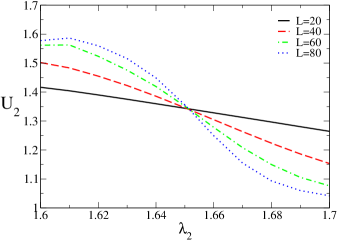
Figure 3: Moment ratio $U_{2}$ versus $\lambda_{2}$ for distinct L‘s and $\lambda_{1}=0.01$.

In fact, as shown in Fig. 4, for $\lambda_{2c}=1.6515$ we find the critical exponents $\beta/\nu_{\perp}=0.794(2)$ and $\beta=0.584(2)$, which are compatible with the DP values (solid lines). Results for other critical points (not shown) confirm that the second-order transitions between the $ab$ and $as$ phases belong to the DP universality class.

Figure 4: In the left, log-log plot of $\rho$ vs $L$ for $\lambda_{1}=0.01$ and $\lambda_{2c}=1.6515$. In the right, log-log plot of $\rho$ vs $y=\lambda_{2}-\lambda_{2c}$ for $\lambda_{1}=0.01$ and $L=80$. The left and right curves have slopes $\beta/\nu_{\perp}=0.796(9)$ and $\beta=0.5834(30)$, respectively.

In Fig. 5 we show results for $\lambda_{1}=18$. For $L=80$ and $\lambda_{2}=0.3618$, the probability distribution $P_{\rho}$ presents two equal peaks at distinct densities ($\rho=0.0002$ and $0.501$) and together a single peak centered at $\phi\sim 0$ for $P_{\phi}$, the phase transition between the $ab$ and $as$ phases for $\lambda_{1}=18$ is first-order.

Figure 5: For the model 1, the quasi-stationary probability distribution $P_{\rho}$ for $\lambda_{1}=18$ and $\lambda_{2}=0.3618$ and $L=80$. In the inset, $P_{\phi}$ for the system density $\phi$.

Next, we study the phase transition between active phases, whose results are exemplified for $\lambda_{1}=0.05$ and shown in Fig. 6. Note that for $2.5<\lambda_{2}<5.0$, $\phi$ has a sharp increase followed by a less pronounced change of $\rho\neq 0$ (inset of Fig. 6), signaling the emergence of the $as-aa$ phase transition. Results for $U_{4}$ show that all curves (for distinct system sizes) cross at $\lambda_{2c}=4.55(5)$ with $U_{4}=0.605(5)$, which is very close to the universal value $U_{4}=0.61069$ and highlighting that such second-order phase transition belongs to the Ising universality class [9]. By increasing further $\lambda_{2}$, $\phi$ reaches a maximum and starting decreasing until vanishing. Such sharp behavior, accompanied by a smooth variation of $\rho$, are consistent to the $aa-as$ phase transition. We see that all cumulant curves cross at $\lambda_{2c}=11.36(5)$ with $U_{4c}=0.60(1)$, which is also consistent with the Ising value. Note that in the $aa$ phase $U_{4}\rightarrow 2/3$ by increasing the system $L$, signaling that the spontaneous symmetry breaking is similar to that found in the Ising model. To confirm above expectations, we analyze the order-parameter variance $\chi$ for finite system sizes, whose results are shown in Fig. 7. At above critical points, we found the exponents $\gamma/\nu=1.75(1)$ and $1.75(1)$, which are in good accordance with the value $7/4$ and hence confirming above expectations.

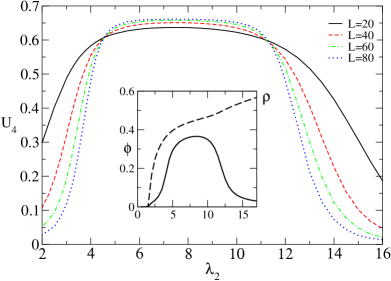
Figure 6: Reduced fourth order cumulant $U_{4}$ versus $\lambda_{2}$ for distinct $L$’s and $\lambda_{1}=0.05$. In the inset, we plot the order-parameter (continuous lines) and the system density $\rho$ (dotted) vs $\lambda_{2}$ for $L=80$.

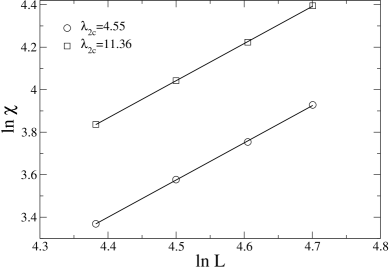
Figure 7: Log-log plot of order-parameter variance $\chi$ versus $L$ for $as-aa$ (circles) and $aa-as$ (squares) for $\lambda_{1}=0.05$. The straight lines have slopes $7/4$.

Figure 8: For the model 2, the phase diagram in the plane $\lambda_{1}-\lambda_{2}$, obtained from MC simulations. Dashed and continuous line denote discontinuous and continuous phase transitions, respectively. The symbols $ab$, $as$, $aa$, $e$ $T$ denote the absorbing, active-symmetric and active-asymmetric phases, critical end point and tricritical points, respectively.

The phase diagram for the model 2 is shown in Fig. 8. In similarity with the model 1 and results by Martins et al., the inclusion of restrictive interaction between next nearest neighbor sites also maintains the $aa$ phase for intermediate values of $\lambda_{2}$. However, confirming some MFT expectations, there are more pronounced differences with respect to above mentioned results. More specifically, the phase $as$ exists solely to larger values of $\lambda_{1}$, in such a way that no $ab-as$ transition line is presented for low $\lambda_{1}$. Besides, the $aa$ phase is constrained by transition lines that are first-order and become critical by increasing $\lambda_{1}$. Hence, in contrast with above mentioned results, the symmetry breaking occurs through a discontinuous phase transition for low $\lambda_{1}$. Also unlike previous cases, tricritical points separate the $as-aa$ and $aa-as$ coexistence lines from those respective critical curves. As a result of restrictive interaction between next-nearest neighbor particles, the $aa$ phase extends for very larger values of control parameters than model 1 and those from Ref. [9]. Also confirming the MFT expectations, the phase transition between $ab$ and $as$ phases is critical and become discontinuous by lowering $\lambda_{1}$. Despite above similarities, remarkable differences with MFT results are presented. There is no triple point in which $ab$, $as$ and $aa$ phases coexist. Instead, the critical $as-aa$ line meets the coexistence line $ab-aa$ in a critical end point $(e)$ (located at $[\lambda_{1},\lambda_{2}]=[0.58(1),7.37(1)]$), giving rise to the $ab-as$ phase coexistence. Besides, the $aa$ phase extends for much larger $\lambda_{2}$ and lower $\lambda_{1}$ than those obtained from MFT, but the critical line $ab-as$ extends for larger values of $\lambda_{1}$ than MFT predictions.

Figure 9: For $L=80$ and $\lambda_{1}=0.5$, in $(a)$ the order parameter $\phi$ (continuous lines) and the system density $\rho$ (dashed lines) vs $\lambda_{2}$. In $(b)$ and $(c)$ probability distributions $P_{\phi}$ and $P_{\rho}$ (inset) for $\lambda_{2}=6.39$ and $\lambda_{2}=50.96$, respectively.

In order to exemplify all above features of the phase diagram, now we show explicit results for distinct points of the phase diagram. Starting from the $ab-aa$ and $aa-as$ coexisting phases, in Fig. 9 we show explicit results for $\lambda_{1}=0.5$. For low $\lambda_{2}$ the system is constrained in the $ab$ phase and at a threshold value ($\lambda_{2}\sim 6.39(1)$ for $\lambda_{1}=0.5$), both $\rho$ and $\phi$ changes abruptly, signaling the $ab-aa$ phase coexistence. As for the model 1, in the $aa$ phase $\rho$ presents a smooth variation, implying that the change of $\phi$ as $\lambda_{2}$ increases comes mainly from the spatial redistribution of particles in sublattices. In addition, the $aa$ phase extends for expressively larger values of $\lambda_{2}$. Probability distributions in Fig. 9$(b)$ reinforce the $ab-aa$ phase transition to be first-order, with two peaks (centered at $\phi\sim 0$ and $\phi\sim 0.25$ for $P_{\phi}$ and $\rho\sim 0$ and $\rho\sim 0.4$ for $P_{\rho}$), in consistency with the observed jumps. At a second threshold value ($\lambda_{2}=50.96(1)$ for $\lambda_{1}=0.5$) $\phi$ vanishes abruptly (with $\rho$ presenting a certain increase), signaling the $aa-as$ phase transition. Once again, probability distributions in Fig. 9$(c)$ confirm such transition to be first-order, with two peaks centered at $\phi\sim 0$ and $\phi\sim 0.45$ ($\rho\sim 0.52$ and $\rho\sim 0.73$) for $P_{\phi}$ ($P_{\rho}$).

Similar above behaviors are verified for other values of $\lambda_{2}$. Numerical results show that $aa-as$ transition lines become critical at $(\lambda_{1},\lambda_{2})$= $(0.65(3),44(1))$. In Fig. 10 we show results for $\lambda_{1}=0.9$, in order to exemplify the second-order transition between active phases. In the interval $10<\lambda_{2}<15$ $\phi$ increases substantially followed by small variation of $\rho\neq 0$. The first crossing curves for $U_{4}$ occurs at $13.65(5)$ with $U_{4}=0.61(1)$, which is consistent with a second-order Ising phase transition. The maximum value of $\phi$ (for $\lambda_{1}=0.9$) yields at $\lambda_{2}\sim 25$, from which $\phi$ starts decreasing until vanishing and no pronounced changes of $\rho$, signals the $aa-as$ phase transition. For such transition, all reduced cumulant $U_{4}$ curves cross in the interval $34.5(2)$ with $U_{4}=0.59(2)$-also consistent with previous phase transitions. By measuring the critical exponents, we obtain in both cases values consistent with the value $7/4$, in similarity with previous results.

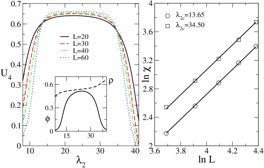
Figure 10: In the left, $U_{4}$ vs $\lambda_{2}$ for distinct system sizes for $\lambda_{1}=0.9$. In the inset, black and dashed lines show the order parameter $\phi$ and system density $\rho$ vs $\lambda_{2}$ for $L=80$, respectively. In the right, log-log plot of $\chi$ vs $L$ at the $as-aa$ (circles) and $aa-as$ (squares) critical points. The straight lines have slopes $7/4$.

In the last analysis, we examine the transition between the absorbing and active (symmetric) phases, whose results are exemplified in Fig. 11 for $\lambda_{1}=1.5$. The probability distribution $P_{\rho}$ has equal height peaks centered at densities $\rho\sim 0$ and $\rho\sim 0.317$, and together the single peak of $P_{\phi}$ centered at $\phi\sim 0$, such result confirms the $ab-as$ phase coexistence for $\lambda_{1}=1.5$.

Figure 11: Quasi-stationary order-parameter probability distribution $P_{\rho}$ for $\lambda_{1}=1.5$ and $L=80$. In the inset, the $P_{\phi}$ for the order-parameter $\phi$.

Finally, we plot results for $\lambda_{1}=3$, in order to exemplify the critical $ab-as$ transition. As shown previously for the model 1, all $U_{2}$ curves cross at the point $\lambda_{2c}=0.602(2)$ with $U_{2}=1.34(1)$, which is close to the DP value $1.3257(5)$. At the above crossing point, $\rho$ behaves algebraically with an exponent consistent with the DP value $\beta/\nu_{\perp}=0.796(9)$, illustrating that the critical $ab-as$ line belongs to the DP universality class.

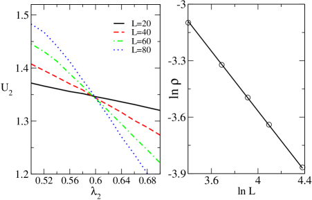
Figure 12: In the left, moment ratio $U_{2}$ versus $\lambda_{2}$ for $\lambda_{1}=3$ and distinct system sizes. In the right, log-log plot of $\rho$ vs $L$ at the transition point $\lambda_{2c}=0.602$. The straight line has slope $\beta/\nu_{\perp}=0.796(9)$.

4 Conclusions

The original two-dimensional contact process with creation at both nearest and next-nearest neighbors and particle suppression exhibit a novel phase structure presenting a continuous phase transition with spontaneous broken-symmetry phase and sublattice ordering [9]. Aimed at exploiting the robustness of such asymmetric phase and the possibility of distinct phase transitions, in this paper we studied the effect of distinct sublattice interactions (instead of only distinct creation rates as in the original model). Two distinct models were considered. In both cases, results confirm that the competition between first and second-neighbor creation rates and particle suppression are fundamental requirements for the presence of an asymmetric active phase. In addition, the inclusion of distinct competing interactions lead to novel phase structures, summarized as follows: A restrictive interaction between nearest neighbor sites (model 1) changes the absorbing phase transition (in contrast with the original model), but not the asymmetric phase. More pronounced changes are found by taking the restrictive interaction between second-neighbor particles (model 2). It not only prolongs greatly the asymmetric phase under larger values of control parameters but also shift the phase transitions, from continuous to discontinuous, even between the active phases. This latter result is particularly interesting since it reinforces the role of restrictive interactions as a minimal mechanism for the appearance of first-order phase transitions [7]. Initially studied for absorbing phase transitions, our results revealed that this ingredient is more general, changing the nature of distinct phases structures. Although predicted by the mean field theory, it is worth mentioning that discontinuous absorbing transitions under the studied restrictive interactions do not occur in one-dimensional systems [15]. The resemblance between $as-aa$ and ferromagnetic-paramagnetic Ising model transition also provides a reasoning why such transitions can not occur in one-dimension. In fact, results obtained by Martins et al. for the original version confirm this. As a final remark, we note that possible extensions of the present work includes exploiting the influence of distinct dynamics (such as diffusion, annihilation rules) in the asymmetric phase. This should be addressed in a ongoing work.

5 Acknowledgments

The authors wish to thank Brazilian scientific agency CNPq, INCT-FCx for the financial support and Universidade Federal do Paraná (UFPR) for providing basic infrastructure to conduct the work. Salete Pianegonda also wishes to thank the Physics Department of the Federal Technological University, Paraná (DAFIS-CT-UTFPR) for providing the access to its high-performance computing facility.

References

References

- [1] J. Marro and R. Dickman, Nonequilibrium Phase Transitions in Lattice Models (Cambridge University Press, Cambridge, England, (1999).
- [2] G. Odor, Rev. Mod. Phys 76, 663 (2004).
- [3] K. A. Takeuchi, M. Kuruda, H. Chaté and M. Sano, Phys. Rev. Lett. 99, 234503 (2007).
- [4] M. Henkel, H. Hinrichsen and S. Lubeck, Non-Equilibrium Transitions, Volume 1 (Springer, 2008).
- [5] See for example, T. Vojta and M. Dickison, Phys. Rev. E 72, 036126 (2005); H. Barghathi and T. Vojta, Phys. Rev. Lett 109, 170603 (2012).
- [6] See for example, J. M. G. Vilar and R. V. Solé, Phys. Rev. E 80, 18 (1998).
- [7] C. E. Fiore, Phys. Rev. E 89, 022104 (2014).
- [8] R. Dickman, Phys. Rev. B 40, 7005 (1989).
- [9] M. M. de Oliveira and R. Dickman, Phys. Rev. E 84, 011125 (2011).
- [10] T. E. Harris, Ann. Probab. 2, 969 (1974).
- [11] E. F. da Silva and M. J. de Oliveira, Comp. Phys. Comm. 183, 2001 (2012).
- [12] M. M. de Oliveira and R. Dickman, Phys. Rev. E, 357, 016129 (2005).
- [13] K. Binder, Phys. Rev. Lett. 47, 693 (1981).
- [14] R. Dickman, Phys. Rev. E 60, R2441 (1999).
- [15] H. Hinrichsen, cond-mat/0006212.