A posteriori error estimates for fully discrete fractional-step $\vartheta$-approximations for the heat equation

Abstract.

We derive optimal order a posteriori error estimates for fully discrete approximations of the initial-boundary value problem for the heat equation. For the discretization in time we apply the fractional-step $\vartheta$-scheme and for the discretization in space the finite element method with finite element spaces that are allowed to change with time. The first optimal order a posteriori error estimates in $L^{\infty}(0,T;L^{2}(\varOmega))$ are derived by applying the reconstruction technique.

1. Introduction

Let $\varOmega$ be a bounded polyedral domain in ${{R}}^{d},d=2,3,$ with boundary $\partial\varOmega$ and $T>0.$ In the present paper we derive optimal order a posteriori error estimates in $L^{\infty}(0,T;L^{2}(\varOmega))$ for fully discrete fractional-step $\vartheta$-scheme approximations for the heat equation:

(1.1) $$\left\{\begin{aligned} &u_{t}-\varDelta u=f\quad&&\text{ \rm{in} }\varOmega\times(0,T],\\ &u=0\quad&&\text{ \rm{on} }\partial\varOmega\times(0,T],\\ &u(x,0)=u^{0}(x)\quad&&\text{ \rm{in} }\varOmega.\\ \end{aligned}\right.$$

We assume throughout that $f\in L^{2}(0,T;L^{2}(\varOmega))$ and $u^{0}\in H_{0}^{1}(\varOmega);$ then the weak solution $u$ of (1.1) belongs to $L^{\infty}(0,T;H_{0}^{1}(\varOmega))$ with $\partial_{t}u\in L^{2}(0,T;L^{2}(\varOmega)).$

Adaptive finite element methods are a fundamental numerical tool in computational science and engineering for approximating partial differential equations with solutions that exhibit nontrivial characteristics. They aim to automatically adjust the mesh to fit the numerical solution, that means fine meshes in the regions where the solution changes fast and coarse in the regions where the solution changes slowly and, consequently, to keep the computational cost as low as possible. The general structure of a loop of an adaptive algorithm for evolution equations is: Given the approximation $U^{n}\in V_{n}$ (reflecting the space discretization method)

1 :

choose the next time node $t^{n+1}$ and the next space $V_{n+1},$

2 :

project $U^{n}$ to $V_{n+1}$ to get $\tilde{U}^{n},$

3 :

use $\tilde{U}^{n}$ as starting value to perform the evolution step in $V_{n+1}$ to obtain the new approximation $U^{n+1}\in V_{n+1}\,.$

The design of such algorithms, particularly the decision made at the first step of the loop, is usually based on suitable a posteriori error estimates which can measure the quality of the approximate solution and provide information of the error distribution.

Although the fractional-step $\vartheta$-scheme was first proposed as an operator splitting method in the context of time-dependent Navier–Stokes equations, cf. [7], [8], and [4], it is an attractive alternative to popular time-stepping schemes, cf. [20], [9]. Indeed, its parameters can be chosen such that to produce a strongly A-stable and second order accurate method. Thus, the scheme can combine the second-order accuracy of the Crank–Nicolson method with the full smoothing property of the backward Euler method in the case of non-smooth initial data. Moreover, in contrast to the backward Euler, it is very little numerically dissipative and, compared to the Runge–Kutta methods of higher order, of lower complexity and storage requirements. For more details we refer to [17], [16], [20], [9] and the references therein.

Despite the great deal of effort that has been devoted to the a posteriori error analysis of linear or nonlinear parabolic equations, cf., for example, [10], [5], [6], [18], [14], [24], [1], [12], [2], the results in case of the fractional-step $\vartheta$-scheme are limited, to our knowledge at least, cf. [11], [15]. Particularly, a posteriori error estimates of optimal order in $L^{\infty}(0,T;L^{2}(\varOmega))$ were derived for time-discrete approximations of linear parabolic equation in [11]. The key for the a posteriori error analysis was the use of a continuous piecewise quadratic in time approximation of $u,$ the so-called fractional-step $\vartheta$-reconstruction, whose residual was second order accurate. The definition of the fore-mentioned reconstruction followed the idea of the two-point Crank-Nicolson reconstruction, cf., [1].

Here, following the ideas developed in [2, 3], we combine the fractional-step $\vartheta$-scheme and the Galerkin finite element method to get a fully discrete scheme consistent with the mesh modification. The first optimal order a posteriori error estimate in $L^{\infty}(0,T;L^{2}(\varOmega))$ for fully fractional-step $\vartheta$-approximations are derived by exploiting both the elliptic reconstruction, cf. [14], and time-reconstruction techniques, cf. [1], [11] and [13]. In particular, we define a continuous representation $\hat{\omega},$ $\hat{\omega}:[0,T]\rightarrow H_{0}^{1}(\varOmega),$ of the approximate solution $U$ which will be referred to as space-time reconstruction of $U.$ The space-time reconstruction $\hat{\omega}$ is a piecewise quadratic polynomial in time which is based on approximations on either one time subinterval or two adjacent time subintervals. Then, the total error $e:=u-U$ may be split as

$$e=u-U=(u-\hat{\omega})+(\hat{\omega}-U)=:\hat{\rho}+\varepsilon,$$

where

1. the space-time reconstruction error $\varepsilon$ may be split as the sum of the elliptic reconstruction error and the time reconstruction error. The elliptic reconstruction error can be bounded by using any elliptic estimator at our disposal and the time reconstruction error can be controlled by a posteriori quantities of optimal order.

2. the parabolic error $\hat{\rho}$ satisfies an appropriate heat equation whose right hand-side can be bounded by computable quantities of optimal order.

The rest of the paper is organized as follows. In Section 2 we introduce notation and the fully discrete scheme allowing mesh change. In Section 3 we first discuss the space- and time-discretization and the corresponding reconstructions and then we present the space-time reconstruction. Specific choices of the reconstructions leading to estimators based on approximations on one time subinterval and on two adjacent time subintervals are given. Section 4 is devoted to the error analysis of the parabolic error $\hat{\rho}$ and we state the final estimates in both aforementioned cases of time-space reconstructions. The asymptotic behavior of the derived estimators is presented in Section 5.

2. Preliminaries

In this section we introduce the necessary notation for our analysis and the fully discrete scheme.

2.1. Notation

Let $0=t^{0}<t^{1}<\cdots<t^{N}=T,$ $I_{n}:=(t^{n-1},t^{n}]$ and $k_{n}:=t^{n}-t^{n-1}.$ For $\vartheta\in(0,\frac{1}{3}),$ $\tilde{\vartheta}=1-2\vartheta,$ we introduce the intermediate time levels $t^{n-1+\vartheta}=t^{n-1}+\vartheta k_{n}$ and $t^{n-\vartheta}=t^{n-1}+(\vartheta+\tilde{\vartheta})k_{n}.$

For each $0\leq n\leq N,$ let $\mathcal{T}_{n}$ be a triangulation of $\varOmega$ into disjoint $d$-simplices $K$ and $h_{n}$ its local mesh-size function defined by

(2.1) $$h_{n}(x):=\text{diam}(K),\quad K\in\mathcal{T}_{n}\text{ and }x\in K.$$

We assume that the aspect ratios of all the elements are uniformly bounded with respect to $n=0,\ldots,N,$ and the intersection of two different elements is either empty, or consists of a common vertex, a common edge, or a common face.

We associate with each $\mathcal{T}_{n}$ a finite element space ${{V}}_{h}^{n}$

(2.2) $$\mathaccent 869{{V}}_{h}^{n}:=\{\phi\in H^{1}(\varOmega):\forall K\in\mathcal{T}_{n}:\phi|_{K}\in{P}^{l}\}\quad\text{and}\quad{{V}}_{h}^{n}:=\mathaccent 869{{V}}_{h}^{n}\cap H_{0}^{1}(\varOmega),$$

where ${P}^{l}$ is the space of polynomials in $d$ variables of degree at most $l.$

For each $n$ and for each $K\in\mathcal{T}_{n},$ we denote by $\mathcal{E}_{n}(K)$ the set of the facets of $K$ and by $\varSigma_{n}(K)\subset\mathcal{E}_{n}(K)$ the set of the interior facets of $K,$ that is the facets that do not belong to the boundary of $\varOmega.$ In addition, we introduce the sets $\mathcal{E}_{n}:=\cup_{K\in\mathcal{T}_{n}}\mathcal{E}_{n}(K)$ and $\varSigma_{n}:=\cup_{K\in\mathcal{T}_{n}}\varSigma_{n}(K)$.

We also make the assumption that all triangulations are derived from the same macro-triangulation by using an admissible refinement procedure, e.g., the bisection-based refinement procedure used in ALBERTA-FEM toolbox, cf. [21]. Given two successive triangulations $\mathcal{T}_{n-1}$ and $\mathcal{T}_{n},$ we define the finest common coarsening $\hat{\mathcal{T}}_{n}:=\mathcal{T}_{n-1}\wedge\mathcal{T}_{n}$ and the coarsest common refinement $\check{\mathcal{T}}_{n}:=\mathcal{T}_{n-1}\vee\mathcal{T}_{n},$ whose local mesh-sizes are given by $\hat{h}_{n}:=\max(h_{n},h_{n-1})$ and $\check{h}_{n}:=\min(h_{n},h_{n-1}),$ respectively. Note that essentially $\hat{\mathcal{T}}_{n}$ is the triangulation of ${{V}}_{h}^{n}\cap{V}_{h}^{n-1}$ and $\check{\mathcal{T}}_{n}$ is the triangulation of ${{V}}_{h}^{n}\cup{{V}}_{h}^{n-1}.$ In addition, we shall denote by $\check{\varSigma}_{n}$ and $\hat{\varSigma}_{n}$ the sets of the interior facets which correspond to $\check{\mathcal{T}}_{n}$ and $\hat{\mathcal{T}}_{n},$ respectively, namely $\check{\varSigma}_{n}:=\cup_{K\in\check{\mathcal{T}}_{n}}\varSigma_{n}(K)$ and $\hat{\varSigma}_{n}:=\cup_{K\in\hat{\mathcal{T}}_{n}}\varSigma_{n}(K).$ We refer to [12] for precise definitions.

We shall use the shorthand notation $u^{m}(\cdot):=u(\cdot,t^{m})$ and $f^{m}(\cdot):=f(\cdot,t^{m})$ throughout. The jump $J[\bm{v}]_{e}$ of a discontinuous vector valued function $\bm{v}$ across an interior facet $e\in\varSigma_{n}(K)$ is defined by

(2.3) $$J[\bm{v}]_{e}(x):=\lim_{\delta\rightarrow 0}[\bm{v}(x+\delta\bm{n}_{e})-\bm{v}(x-\delta\bm{n}_{e})]\cdot\bm{n}_{e},$$

where $\bm{n}_{e}$ is a unit normal vector on $e$ and $x\in e.$

We denote by ${\langle}\cdot,\cdot{\rangle}$ either the inner product in $L^{2}(\varOmega)$ or the duality pairing between $H^{-1}(\varOmega)$ and $H_{0}^{1}(\varOmega)$ and we let $a(\cdot,\cdot)$ be defined as $a(u,v):={\langle}\nabla u,\nabla v{\rangle}.$ For $\mathcal{D}\subset\mathbb{R}^{d}$ we denote by $\|\cdot\|_{\mathcal{D}}$ the norm in $L^{2}(\mathcal{D}),$ by $\|\cdot\|_{r,\mathcal{D}}$ and by $|\cdot|_{r,\mathcal{D}}$ the norm and the semi-norm, respectively, in the Sobolev space $H^{r}(\mathcal{D}),r\in\mathbb{N}.$ In view of the Poincaré inequality, we consider $|\cdot|_{1,\mathcal{D}}$ to be the norm in $H_{0}^{1}(\mathcal{D})$ and denote by $|\cdot|_{-1,\mathcal{D}}$ the norm in $H^{-1}(\mathcal{D});$ whenever $\mathcal{D}=\varOmega$ the subscript $\mathcal{D}$ will be omitted in the notation of function spaces and norms.

In addition, we shall use the following notation for functions $v$ defined in a piecewise sense

(2.4) $$\|h_{n}^{i}v\|_{\mathcal{T}_{n}} =\left(\sum_{K\in\mathcal{T}_{n}}\|h_{K}^{i}v\|_{K}^{2}\right)^{1/2}$$

$$\quad\text{and}\quad\|h_{n}^{i+\frac{1}{2}}J[\nabla v]\|_{\varSigma_{n}} =\left(\sum_{e\in\varSigma_{n}}\|h_{e}^{i+\frac{1}{2}}J[\nabla v]_{e}\|^{2}_{e}\right)^{1/2},\quad i=1,2.$$

2.2. Discrete operators and interpolants

For $0\leq n\leq N,$ let $\varDelta_{h}^{n}:H_{0}^{1}\rightarrow{{V}}_{h}^{n}$ be the discrete Laplacian corresponding to the finite element space ${{V}}_{h}^{n}$ defined by

(2.5) $${\langle}(-\varDelta_{h}^{n})v,\chi_{n}{\rangle}={\langle}\nabla v,\nabla\chi_{n}{\rangle}\quad\forall\chi_{n}\in{{V}}_{h}^{n}.$$

Moreover, we denote by $P_{0}^{n},$ $P_{0}^{n}:L^{2}\rightarrow{{V}}_{h}^{n},$ the $L^{2}$-projection onto ${{V}}_{h}^{n}$ and, in order our analysis to include several possible choices for the projection step, $\varPi^{n},\mathaccent 869{\varPi}^{n}:{V}_{h}^{n-1}\rightarrow{V}_{h}^{n}$ will denote appropriate projections or interpolants to be chosen.

We now recall the stability property and the approximation properties of the Clément-type interpolant introduced in [22].

Lemma 2.1.

Let $\mathcal{I}^{n}:H_{0}^{1}\rightarrow{V}_{h}^{n}$ be a Clément-type interpolant. Then, we have

(2.6) $$|\mathcal{I}^{n}z|_{1}\leq c_{1}|z|_{1}.$$

Furthermore, for $j\leq l+1,$ the following approximation properties are satisfied

(2.7) $$\|h_{n}^{-j}(z-\mathcal{I}^{n}z)\|_{\mathcal{T}^{n}}\leq c_{1,j}|z|_{j},$$

$$\|h_{n}^{1/2-j}(z-\mathcal{I}^{n}z)\|_{\varSigma_{n}}\leq c_{2,j}|z|_{j},$$

where $l$ is the finite element polynomial degree and the constants $c_{1},$ $c_{1,j}$ and $c_{2,j}$ depend only on the shape-regularity of the family of triangulations $\{\mathcal{T}_{n}\}_{n=0}^{N}.$ ∎

Let $C_{E}$ denote the elliptic regularity constant, that is

(2.8) $$|v|_{2}\leq C_{E}\|\varDelta v\|,\quad v\in H^{2}(\varOmega)\cap H^{1}_{0}(\varOmega)\,,$$

and $c_{1},$ $c_{i,j},i=1,2,\;j\leq l+1,$ be the constants in Lemmas 2.1. We shall also use the notation

$$C_{j,2}:=C_{E}\,c_{j,2}\,$$

for the constants appeared in the definition of the a posteriori error estimators.

2.3. The fully discrete scheme

We discretize (1.1) by applying the following Galerkin fractional-step $\vartheta$-scheme (GFS-scheme): for a given approximation $U^{0}$ of $u^{0}$ and for $1\leq n\leq N,$ find $U^{n}\in{{V}}_{h}^{n},$ such that

(2.9) $$\left\{\begin{aligned} &\frac{U^{n-1+\vartheta}-\varPi^{n}U^{n-1}}{\vartheta k_{n}}-\alpha_{1}\varDelta_{h}^{n}U^{n-1+\vartheta}-\beta_{1}\mathaccent 869{\varPi}^{n}\varDelta_{h}^{n-1}U^{n-1}=P_{0}^{n}\{\alpha_{2}f^{n-1+\vartheta}+\beta_{2}f^{n-1}\},\\ &\frac{U^{n-\vartheta}-U^{n-1+\vartheta}}{\tilde{\vartheta}k_{n}}-\beta_{1}\varDelta_{h}^{n}U^{n-\vartheta}-\alpha_{1}\varDelta_{h}^{n}U^{n-1+\vartheta}=P_{0}^{n}\{\beta_{2}f^{n-\vartheta}+\alpha_{2}f^{n-1+\vartheta}\},\\ &\frac{U^{n}-U^{n-\vartheta}}{\vartheta k_{n}}-\alpha_{1}\varDelta_{h}^{n}U^{n}-\beta_{1}\varDelta_{h}^{n}U^{n-\vartheta}=P_{0}^{n}\{\alpha_{2}f^{n}+\beta_{2}f^{n-\vartheta}\},\end{aligned}\right.$$

with $\alpha_{1},\alpha_{2}\in(0,1),$ and $\beta_{1}=1-\alpha_{1},\beta_{2}=1-\alpha_{2}.$ We shall sometimes find it convenient to rewrite (2.9) in the form

(2.10) $$\left\{\begin{aligned} &\frac{U^{n-1+\vartheta}-\varPi^{n}U^{n-1}}{k_{n}}-\bigl{\{}\alpha_{1}\vartheta\varDelta_{h}^{n}U^{n-1+\vartheta}+\beta_{1}\vartheta\mathaccent 869{\varPi}^{n}\varDelta_{h}^{n-1}U^{n-1}\bigr{\}}\\ =&P_{0}^{n}\bigl{\{}\alpha_{2}\vartheta f^{n-1+\vartheta}+\beta_{2}\vartheta f^{n-1}\bigr{\}},\\ &\frac{U^{n-\vartheta}-\varPi^{n}U^{n-1}}{k_{n}}-\bigl{\{}\beta_{1}\tilde{\vartheta}\varDelta_{h}^{n}U^{n-\vartheta}+\alpha_{1}(\vartheta+\tilde{\vartheta})\varDelta_{h}^{n}U^{n-1+\vartheta}+\beta_{1}\vartheta\mathaccent 869{\varPi}^{n}\varDelta_{h}^{n-1}U^{n-1}\bigr{\}}\\ =&P_{0}^{n}\bigl{\{}\beta_{2}\tilde{\vartheta}f^{n-\vartheta}+\alpha_{2}(\vartheta+\tilde{\vartheta})f^{n-1+\vartheta}+\beta_{2}\vartheta f^{n-1}\bigr{\}},\\ &\frac{U^{n}-\varPi^{n}U^{n-1}}{k_{n}}-\bigl{\{}\alpha_{1}\vartheta\varDelta_{h}^{n}U^{n}+\beta_{1}(\vartheta+\tilde{\vartheta})\varDelta_{h}^{n}U^{n-\vartheta}+\alpha_{1}(\vartheta+\tilde{\vartheta})\varDelta_{h}^{n}U^{n-1+\vartheta}\\ &+\beta_{1}\vartheta\mathaccent 869{\varPi}^{n}\varDelta_{h}^{n-1}U^{n-1}\bigr{\}}\\ =&P_{0}^{n}\bigl{\{}\alpha_{2}\vartheta f^{n}+\beta_{2}(\vartheta+\tilde{\vartheta})f^{n-\vartheta}+\alpha_{2}(\vartheta+\tilde{\vartheta})f^{n-1+\vartheta}+\beta_{2}\vartheta f^{n-1}\bigr{\}}.\end{aligned}\right.$$

Throughout the rest of the paper we shall assume that $\vartheta=1-\frac{\sqrt{2}}{2}$ and $\alpha_{1}\in(\frac{1}{2},1],$ which implies that the fractional-step $\vartheta$-scheme is second-order accurate and $A(0)$-stable. Indeed, the assumption that $\alpha_{1}\in(\frac{1}{2},1]$ implies the strong $A$-stability of our scheme. Furthermore, we can easily seen that the quadrature rule

(2.11) $$\mathcal{I}_{\alpha,\vartheta}(\phi):=\beta\vartheta\phi(0)+\alpha(\vartheta+\tilde{\vartheta})\phi(\vartheta)+\beta(\vartheta+\tilde{\vartheta})\phi(1-\vartheta)+\alpha\vartheta\phi(1)\approx\int_{0}^{1}\phi(s)ds$$

integrates first degree polynomials exactly if and only if $\alpha=\beta=\frac{1}{2}$ or $\vartheta=1-\frac{\sqrt{2}}{2}$. Thus, the assumption $\vartheta=1-\frac{\sqrt{2}}{2}$ ensures that the fractional-step $\vartheta$-scheme is second-order accurate with respect to time. We refer to [9] for more details.

2.4. The fully discrete scheme in compact form

We introduce the following piecewise linear polynomials with respect to time

(2.12) $$\varphi(t):=\ell_{0}^{n}(t)f^{n-1}+\ell_{1}^{n}(t)f^{n},\quad t\in I_{n},$$

and

(2.13) $$\varTheta(t)=\ell_{0}^{n}(t)\mathaccent 869{\varPi}^{n}(-\varDelta_{h}^{n-1})U^{n-1}+\ell_{1}^{n}(t)(-\varDelta_{h}^{n})U^{n},\quad t\in I_{n},$$

with

(2.14) $$\ell_{0}^{n}(t):=\frac{t^{n}-t}{k_{n}}\quad\text{and}\quad\ell_{1}^{n}(t):=\frac{t-t^{n-1}}{k_{n}},\quad t\in I_{n}.$$

Moreover, we let $\hat{\varTheta}$ be defined as

(2.15) $$\mathaccent 866{\varTheta}(t):=\varTheta(t)-\xi_{\varTheta}^{n},\quad t\in I_{n},$$

with

(2.16) $$\xi_{\varTheta}^{n}:=(\vartheta+\tilde{\vartheta})\bigl{\{}\alpha[\varTheta(t^{n-1+\vartheta})+\varDelta_{h}^{n}U^{n-1+\vartheta}]+\beta[\varTheta(t^{n-\vartheta})+\varDelta_{h}^{n}U^{n-\vartheta})]\bigr{\}},\quad t\in I_{n},$$

and $\hat{\varphi}$

(2.17) $$\hat{\varphi}(t):=\varphi(t)-\xi_{\varphi}^{n},\quad t\in I_{n},$$

with

(2.18) $$\xi_{\varphi}^{n}:=(\vartheta+\tilde{\vartheta})\bigl{\{}\alpha[\varphi(t^{n-1+\vartheta})-f^{n-1+\vartheta}]+\beta[\varphi(t^{n-\vartheta})-f^{n-\vartheta})]\bigr{\}},\quad t\in I_{n}.$$

Note that both $\xi_{\varTheta}^{n}$ and $\xi_{\varphi}^{n}$ are a posteriori quantities of optimal order, cf. [11] for details.

According to definitions (2.15) and (2.17) the last substep of the fractional-step $\vartheta$-scheme may be written in the following compact form

(2.19) $$\frac{U^{n}-\varPi^{n}U^{n-1}}{k_{n}}+\mathaccent 866{\varTheta}(t^{n-\frac{1}{2}})=P_{0}^{n}\hat{\varphi}(t^{n-\frac{1}{2}}).$$

3. Space-time reconstructions

As aforementioned, the a posteriori error estimates will be derived by using the reconstruction technique. Our goal is to define a continuous representation $\hat{\omega}$ of the approximate solution, $\hat{\omega}:[0,T]\rightarrow H_{0}^{1}(\varOmega),$ which will be a second order approximation of the exact solution $u(t)$ and whose residual will also be second order accurate. To define $\hat{\omega}(t)$ we shall exploit both the ideas of elliptic reconstruction introduced in [14] and the fractional-step $\vartheta$-reconstruction based on approximations on one time subinterval introduced in [11]. Additionally, we shall extend the idea of the three-point Crank–Nicolson reconstruction introduced in [13, 19] and shall define a second fractional-step $\vartheta$-reconstruction which will be based on approximations on two adjacent time subintervals. We shall begin our discussion by recalling the definition of the elliptic reconstruction operator and its basic properties.

3.1. Reconstruction in space

To derive a posteriori error estimates of optimal order in $L^{\infty}(0,T;L^{2}(\varOmega))$ norm for finite element discretizations of parabolic equations, the use of the elliptic reconstruction is necessary. The elliptic reconstruction may be regarded as an a posteriori analogue to the Ritz–Wheeler projection appearing in standard a priori error analysis for parabolic problems, c.f., for example, [25], [23]. Note that in fully discrete case with finite element spaces allowed to change with time the elliptic reconstruction operator depends on $n.$

Definition 3.1 (Elliptic reconstruction).

For fixed $v_{n}\in{{V}}_{h}^{n}$, we define the elliptic reconstruction ${\mathcal{R}}^{n}v_{n}\in H_{0}^{1}$ of $v_{n},$ as the solution of the following elliptic problem

(3.1) $${\langle}\nabla{\mathcal{R}}^{n}v_{n},\nabla\psi{\rangle}={\langle}(-\varDelta_{h}^{n})v_{n},\psi{\rangle}\quad\forall\psi\in H_{0}^{1}.$$

It can be easily seen that the elliptic reconstruction ${\mathcal{R}}^{n}$ satisfies the Galerkin orthogonality property

(3.2) $${\langle}\nabla({\mathcal{R}}^{n}v_{n}-v_{n}),\nabla\chi_{n}{\rangle}=0\quad\forall\chi_{n}\in{{V}}_{h}^{n}.$$

For completeness we shall next give a residual-based a posteriori estimate for the elliptic reconstruction error $\|({\mathcal{R}}^{n}-I)v_{n}\|.$

Lemma 3.1 (Residual-based a posteriori estimate for the elliptic reconstruction error).

Let $v_{n}\in{{V}}_{h}^{n}$ and ${\mathcal{R}}^{n}v_{n}$ its elliptic reconstruction defined as in (3.1). Then, it holds

(3.3) $$\|({\mathcal{R}}^{n}-I)v_{n}\|\leq\eta_{n}(v_{n}),$$

where $\eta_{n}$ is the elliptic estimator given by

(3.4) $$\eta_{n}(v_{n}):=C_{1,2}\,\|h_{n}^{2}(\varDelta-\varDelta_{h}^{n})v_{n}\|_{\mathcal{T}_{n}}+C_{2,2}\,\|h_{n}^{3/2}J[\nabla v_{n}]\|_{\varSigma_{n}}\,.$$

Proof.  Let $z\in H_{0}^{1}$ be the solution of problem

(3.5) $$a(\chi,z)={\langle}({\mathcal{R}}^{n}-I)v_{n},\chi{\rangle}\quad\forall\chi\in H_{0}^{1},$$

and $\mathcal{I}^{n}z\in{V}_{h}^{n}$ be a Clément-type interpolant of $z.$ By using (3.5), the orthogonality property of the elliptic reconstruction (3.2) and integration by parts, we get

(3.6) $$\|({\mathcal{R}}^{n}-I)v_{n}\|^{2} =a(({\mathcal{R}}^{n}-I)v_{n},(z-\mathcal{I}^{n}z))$$

$$=\sum_{K\in T_{n}}\int_{K}(\varDelta-\varDelta_{h}^{n})v_{n}(z-\mathcal{I}^{n}z)-\sum_{e\in\varSigma_{n}}\int_{e}J[\nabla v_{n}]\,(z-\mathcal{I}^{n}z).$$

Now, by applying first the approximation properties of the Clément interpolant (2.7) and afterwards the elliptic regularity (2.8), we obtain

$$\sum_{K\in T_{n}}\int_{K}(\varDelta-\varDelta_{h}^{n})v_{n}(z-\mathcal{I}^{n}z) \leq c_{1,2}\,|z|_{2}\,\left(\sum_{K\in\mathcal{T}_{n}}\|h_{K}^{2}(\varDelta-\varDelta_{h}^{n})v_{n}\|_{K}^{2}\right)^{\frac{1}{2}}$$

$$\leq C_{1,2}\,\|({\mathcal{R}}^{n}-I)v_{n}\|\,\|h_{n}^{2}(\varDelta-\varDelta_{h}^{n})v_{n}\|_{\mathcal{T}_{n}}$$

and

$$\sum_{e\in\varSigma_{n}}\int_{e}J[\nabla v_{n}]\,(z-\mathcal{I}^{n}z) \leq c_{2,2}\,|z|_{2}\,\left(\sum_{e\in\varSigma_{n}}\|h_{K}^{\frac{3}{2}}\,J[\nabla v_{n}]\|_{e}^{2}\right)^{\frac{1}{2}}$$

$$\leq C_{2,2}\,\|({\mathcal{R}}^{n}-I)v_{n}\|\,\|h_{n}^{3/2}J[\nabla v_{n}]\|_{\varSigma_{n}}\,.$$

∎

We shall now turn our discussion to the time discretization and the so-called fractional-step $\vartheta$-reconstruction.

3.2. Reconstruction in time

Regarding the temporal variable, our goal is to define a second order approximation $U(t)$ of $u(t),$ for all $t\in[0,T],$ whose residual is also second order accurate. Choosing $U:[0,T]\rightarrow H_{0}^{1}(\varOmega)$ to be the piecewise linear interpolant at the nodal values, that is

(3.7) $$U(t):=\ell_{0}^{n}(t)\,U^{n-1}+\ell_{1}^{n}(t)\,U^{n},\quad t\in I_{n},$$

where $\ell_{0}^{n}$ and $\ell_{1}^{n}$ are defined in (2.14), seems natural for a second-order accurate scheme. Indeed, since the error at the nodes is of second order, $U(t)$ is an approximation of $u(t)$ of the same order, for all $t\in[0,T].$ However, its residual $R_{U}(t)$

(3.8) $$R_{U}(t):=U_{t}(t)-\varDelta U(t)-f(t),\quad t\in I_{n},$$

is an a posteriori quantity of first order with respect to time. We observe, using (1.1), that $R_{U}(t)$ may be written also in the form

(3.9) $$R_{U}(t)=[U_{t}(t)-u_{t}(t)]-\varDelta[U(t)-u(t)],\quad t\in I_{n}\,.$$

Although the second term on the right-hand side is of second order, we note that the first term is of first order only. By applying energy techniques to this error equation we can only derive residual-based a posteriori error estimates of suboptimal order with respect to time.

To recover the second order of accuracy in time, we shall define appropriate reconstructions $\hat{U}$ in time which will be piecewise quadratic polynomials based on approximations on one time subinterval as well as on approximations based on two time subintervals.

Definition 3.2 (Time reconstructions).

We introduce the piecewise quadratic time reconstruction $\hat{U}:[0,T]\rightarrow H_{0}^{1}(\varOmega),$ as follows

(3.10) $$\hat{U}(t)=U(t)+\frac{1}{2}(t-{t^{n-1}})(t-t^{n})w_{n},\quad t\in I_{n},$$

$n=1,\ldots,N,$ where $w_{n}$ is an appropriate piecewise constant polynomial with respect to time.

In view of (3.2), we can easily see that

Lemma 3.2 ($L^{\infty}(L^{2})$-estimate for the time reconstruction error).

For $n=1,\ldots,N,$ the following estimate holds

(3.11) $$\max_{t^{n-1}\leq t\leq t^{n}}\|(\hat{U}-U)(t)\|\leq\frac{k_{n}^{2}}{8}\|w_{n}\|,\quad t\in I_{n}.$$

In the sequel we shall study two choices for the time reconstruction $\hat{U}$ which correspond to two appropriate choices for $w_{n}.$ In particular, we shall consider the following cases:

Time reconstruction 1(based on approximations on one time subinterval):

We shall extend the idea of the fractional-step $\vartheta$-reconstruction introduced in [11] to the fully discrete case. For this purpose we choose $w_{n}$ as

(3.12) $$w_{n}(t):=\varTheta_{t}(t)-P_{0}^{n}\varphi_{t}(t)=\frac{(-\varDelta_{h}^{n})U^{n}-\mathaccent 869{\varPi}^{n}(-\varDelta_{h}^{n-1})U^{n-1}}{k_{n}}-\frac{P_{0}^{n}[f^{n}-f^{n-1}]}{k_{n}},\quad t\in I_{n}.$$

Time reconstruction 2(based on approximations on two adjacent time subintervals):

The so-called three-point quadratic reconstruction for the Crank–Nicolson scheme, [13, 19], is defined by choosing $w_{n}$ to be a finite difference approximation of $u_{tt}$ that uses the approximations on two time subintervals. Based on this idea, we define a three time-level quadratic reconstruction for the GFS-scheme by replacing $w_{n}$ in (3.10) with

(3.13) $$\mathaccent 869{w}_{n}:=-{\frac{2}{k_{n}+k_{n-1}}}\Big{[}\Bigl{(}\frac{U^{n}-\varPi^{n}U^{n-1}}{k_{n}}\Bigr{)}-\pi^{n}\Bigl{(}\frac{U^{n-1}-\varPi^{n-1}U^{n-2}}{k_{n-1}}\Bigr{)}\,\Big{]},\quad t\in I_{n},$$

where $\pi^{n}$ is any projection to ${V}_{h}^{n}$ at our disposal.

3.3. Reconstruction in both space and time

The construction of appropriate space-time reconstructions for our analysis combines the ideas discussed in the previous two paragraphs. Let $\omega:[0,T]\rightarrow H_{0}^{1}$ be the piecewise linear in time function defined by linearly interpolating between the values ${\mathcal{R}}^{n-1}U^{n-1}$ and ${\mathcal{R}}^{n}U^{n},$

(3.14) $$\omega(t):=\ell_{0}^{n}(t){\mathcal{R}}^{n-1}U^{n-1}+\ell_{1}^{n}(t){\mathcal{R}}^{n}U^{n},\quad t\in I_{n},$$

with $\ell_{0}^{n}$ and $\ell_{1}^{n}$ as in (2.14). According to the discussion above, the use of $\omega$ as intermediate function in order to derive a posteriori error estimates will give optimal order estimates with respect the spatial derivative, however it will lead to sub-optimal error estimates with respect the temporal one. The introduction of a piecewise quadratic polynomial in time is necessary, therefore we define the space-time reconstruction $\hat{\omega}$ of the approximate solution $U$:

Definition 3.3 (Space–time reconstruction).

We introduce the space-time reconstruction $\hat{\omega}:[0,T]\rightarrow H_{0}^{1}$ of the approximate solution $U$ as follows

(3.15) $$\hat{\omega}(t)=\omega(t)+\frac{1}{2}(t-t^{n-1})(t^{n}-t){\mathcal{R}}^{n}w_{n}.$$

We shall now derive an $L^{\infty}(L^{2})$-estimate for the space-time reconstruction error $\varepsilon=\hat{\omega}-U.$ The error $\varepsilon$ may be written as the sum of the elliptic reconstruction error $\epsilon$ and the time reconstruction error $\sigma,$ that is

(3.16) $$\hat{\omega}-U=\epsilon+\sigma,\quad\text{where }\epsilon:=\omega-U,\;\sigma:=\hat{\omega}-\omega.$$

According to (3.3) and (3.11) the following upper bounds for the reconstruction errors $\epsilon$ and $\sigma$ are valid.

Lemma 3.3.

For $m=1,\ldots,N,$ the following estimates hold

(3.17) $$\max_{0\leq t\leq t^{m}}\|\epsilon(t)\|\leq{\mathcal{E}}_{m}^{\emph{ell}}\quad\text{with}\quad{\mathcal{E}}_{m}^{\emph{ell}}:=\max_{0\leq n\leq m}\eta_{n}(U^{n})$$

and

(3.18) $$\max_{0\leq t\leq t^{m}}\|\sigma(t)\|\leq{\mathcal{E}}_{m}^{\emph{rec}}(w_{n})\quad\text{with}\quad{\mathcal{E}}_{m}^{\emph{rec}}(w_{n}):=\max_{0\leq n\leq m}\frac{k_{n}^{2}}{8}\bigl{\{}\eta_{n}(w_{n})+\|w_{n}\|\bigr{\}},$$

where $\eta_{n}$ is defined in (3.4).

4. $L^{\infty}(L^{2})$-estimates for the total error

Let $\rho,\;\hat{\rho}$ denote the parabolic errors defined by $\rho:=u-\omega,\;\hat{\rho}:=u-\hat{\omega},$ respectively. The total error $e:=u-U$ can be split as follows

(4.1) $$e=u-U=(u-\hat{\omega})+(\hat{\omega}-U)=\hat{\rho}+\sigma+\epsilon.$$

A bound for the reconstruction error $\sigma+\epsilon$ was presented in the previous section. We shall now continue with the estimation of the basic parabolic error, which is stated in Theorem 4.1.

4.1. An a posteriori estimate in $L^{\infty}(L^{2})$ and $L^{2}(H^{1})$ for the parabolic error

We begin with the derivation of the error equation:

Lemma 4.1 (Error equation).

For each $t\in I_{n},$ it holds

(4.2) $${\langle}\hat{\rho}_{t}(t),\psi{\rangle}+a(\rho(t),\psi)={\langle}R_{h},\psi{\rangle}\quad\forall\psi\in H_{0}^{1},$$

with

(4.3) $$R_{h}:= \ell_{0}^{n}(t)(\varPi^{n}-I)(-\varDelta_{h}^{n-1})U^{n-1}-k_{n}^{-1}(\varPi^{n}-I)U^{n-1}-(t-t^{n-\frac{1}{2}})({\mathcal{R}}^{n}-I)w_{n}$$

$$-(t-t^{n-\frac{1}{2}})(w_{n}-\varTheta_{t}(t)+P_{0}^{n}\varphi_{t}(t))-\frac{({\mathcal{R}}^{n-1}-I)U^{n-1}-({\mathcal{R}}^{n}-I)U^{n}}{k_{n}}$$

$$+\xi_{\varTheta}^{n}+f(t)-P_{0}^{n}\hat{\varphi}(t).$$

Proof.  For $n=1,\ldots,N,$ and $\psi\in H_{0}^{1},$ in view of (3.14) and (3.15), we obtain

(4.4) $${\langle}\hat{\omega}_{t}(t),\psi{\rangle}={\langle}\omega_{t}(t),\psi{\rangle}+(t-t^{n-\frac{1}{2}}){\langle}{\mathcal{R}}^{n}w_{n},\psi{\rangle}.$$

Thus, by using Definition 3.3, we get

$${\langle}\hat{\rho}_{t}(t),\psi{\rangle}+a(\rho(t),\psi)= -a(\ell_{0}^{n}(t){\mathcal{R}}^{n-1}U^{n-1}+\ell_{1}^{n}(t){\mathcal{R}}^{n}U^{n},\psi)-(t-t^{n-\frac{1}{2}}){\langle}{\mathcal{R}}^{n}w_{n},\psi{\rangle}$$

$$-k_{n}^{-1}{\langle}{\mathcal{R}}^{n}U^{n}-{\mathcal{R}}^{n-1}U^{n-1},\psi{\rangle}+{\langle}f(t),\psi{\rangle}$$

According to the elliptic reconstruction definition (3.1), the last relation leads to

(4.5) $${\langle}\hat{\rho}_{t}(t), \psi{\rangle}+a(\rho(t),\psi)=-{\langle}\ell_{0}^{n}(t)(-\varDelta_{h}^{n-1})U^{n-1}+\ell_{1}^{n}(t)(-\varDelta_{h}^{n})U^{n},\psi{\rangle}$$

$$-(t-t^{n-\frac{1}{2}}){\langle}{\mathcal{R}}^{n}w_{n},\psi{\rangle}-k_{n}^{-1}{\langle}{\mathcal{R}}^{n}U^{n}-{\mathcal{R}}^{n-1}U^{n-1},\psi{\rangle}+{\langle}f(t),\psi{\rangle},$$

from which, in view of (2.13), we infer that

(4.6) $${\langle}\hat{\rho}_{t}(t),\psi{\rangle}+a(\rho(t),\psi)= -{\langle}\varTheta(t),\psi{\rangle}+\ell_{0}^{n}(t){\langle}(\varPi^{n}-I)(-\varDelta_{h}^{n-1})U^{n-1},\psi{\rangle}$$

$$-(t-t^{n-\frac{1}{2}}){\langle}({\mathcal{R}}^{n}-I)w_{n},\psi{\rangle}-(t-t^{n-\frac{1}{2}}){\langle}w_{n},\psi{\rangle}$$

$$-k_{n}^{-1}{\langle}({\mathcal{R}}^{n-1}-I)U^{n-1}-({\mathcal{R}}^{n}-I)U^{n},\psi{\rangle}$$

$$+k_{n}^{-1}{\langle}U^{n}-U^{n-1},\psi{\rangle}+{\langle}f(t),\psi{\rangle},$$

Now, in view of (2.19), we observe that

(4.7) $${\langle}\hat{\rho}_{t}(t), \psi{\rangle}+a(\rho(t),\psi)=\ell_{0}^{n}(t){\langle}(\varPi^{n}-I)(-\varDelta_{h}^{n-1})U^{n-1}-k_{n}^{-1}(\varPi^{n}-I)U^{n-1},\psi{\rangle}$$

$$-(t-t^{n-\frac{1}{2}}){\langle}({\mathcal{R}}^{n}-I)w_{n},\psi{\rangle}-(t-t^{n-\frac{1}{2}}){\langle}w_{n},\psi{\rangle}+{\langle}\hat{\varTheta}(t^{n-\frac{1}{2}})-P_{0}^{n}\hat{\varphi}(t^{n-\frac{1}{2}}),\psi{\rangle}$$

$$-k_{n}^{-1}{\langle}({\mathcal{R}}^{n-1}-I)U^{n-1}-({\mathcal{R}}^{n}-I)U^{n},\psi{\rangle}-{\langle}\varTheta(t),\psi{\rangle}+{\langle}f(t),\psi{\rangle}.$$

In view of (2.15) and (2.17) we can easily see that

(4.8) $$\hat{\varTheta}(t^{n-\frac{1}{2}})-P_{0}^{n}\hat{\varphi}(t^{n-\frac{1}{2}})=(t-t^{n-\frac{1}{2}})(\varTheta_{t}(t)-P_{0}^{n}\varphi_{t}(t)),$$

and thus to conclude that

(4.9) $${\langle}\hat{\rho}_{t}(t),\psi{\rangle}+ a(\rho(t),\psi)=\ell_{0}^{n}(t){\langle}(\varPi^{n}-I)(-\varDelta_{h}^{n-1})U^{n-1}-k_{n}^{-1}(\varPi^{n}-I)U^{n-1},\psi{\rangle}$$

$$-(t-t^{n-\frac{1}{2}}){\langle}({\mathcal{R}}^{n}-I)w_{n},\psi{\rangle}-(t-t^{n-\frac{1}{2}}){\langle}w_{n}-\varTheta_{t}(t)+P_{0}^{n}\varphi_{t}(t),\psi{\rangle}$$

$$-k_{n}^{-1}{\langle}({\mathcal{R}}^{n-1}-I)U^{n-1}-({\mathcal{R}}^{n}-I)U^{n},\psi{\rangle}$$

$$+{\langle}\xi_{\varTheta}^{n},\psi{\rangle}+{\langle}f(t)-P_{0}^{n}\hat{\varphi}(t),\psi{\rangle}.$$

∎

An a posteriori error bound for the parabolic error follows. Note that the estimate that we will derive depends still on the choice of the time reconstruction through $w_{n}$ as well as on stationary finite element errors through the elliptic reconstruction ${\mathcal{R}}^{n}.$

Theorem 4.1.

(Estimates in $L^{\infty}(L^{2})$ and $L^{2}(H^{1})$ for the parabolic error)

The following estimate is valid

(4.10) $$\max_{t\in[0,t^{m}]}\bigl{\{}\|\hat{\rho}(t)\|^{2}+\int_{0}^{t}(|\rho(s)|^{2}+|\hat{\rho}(s)|^{2})\,ds\bigr{\}}\leq\,\|\hat{\rho}(0)\|^{2}+\mathcal{J}_{m},$$

where $\mathcal{J}_{m},\,m=1,\ldots,N,$ is defined by

(4.11) $$\mathcal{J}_{m}:=\mathcal{J}_{m}^{T,1}+\mathcal{J}_{m}^{T,2}+\mathcal{J}_{m}^{S,1}+\mathcal{J}_{m}^{S,2}+\mathcal{J}_{m}^{C}+\mathcal{J}_{m}^{D}+\mathcal{J}_{m}^{W},$$

with

(4.12) $$\mathcal{J}_{m}^{T,1}:=\sum_{n=1}^{m}\int_{t^{n-1}}^{t^{n}}|\sigma(s)|^{2}\,ds,$$

(4.13) $$\mathcal{J}_{m}^{T,2}:=2\sum_{n=1}^{m}\int_{t^{n-1}}^{t^{n}}|{\langle}\xi_{\varTheta}^{n},\hat{\rho}(s){\rangle}|ds,$$

(4.14) $$\mathcal{J}_{m}^{S,1}:=2\sum_{n=1}^{m}\int_{t^{n-1}}^{t^{n}}|(s-t^{n-\frac{1}{2}}){\langle}({\mathcal{R}}^{n}-I)w_{n},\hat{\rho}(s){\rangle}|ds$$

(4.15) $$\mathcal{J}_{m}^{S,2}:=2\sum_{n=1}^{m}\int_{t^{n-1}}^{t^{n}}|{\langle}\frac{({\mathcal{R}}^{n}-I)U^{n}-({\mathcal{R}}^{n-1}-I)U^{n-1}}{k_{n}},\hat{\rho}(s){\rangle}|ds$$

(4.16) $$\mathcal{J}_{m}^{C}:=2\sum_{n=1}^{m}\int_{t^{n-1}}^{t^{n}}|{\langle}\ell_{0}^{n}(s)(\mathaccent 869{\varPi}^{n}-I)(-\varDelta_{h}^{n-1})U^{n-1}-k_{n}^{-1}(\varPi^{n}-I)U^{n-1},\hat{\rho}(s){\rangle}|\,ds\,.$$

(4.17) $$\mathcal{J}_{m}^{D}:=2\sum_{n=1}^{m}\int_{t^{n-1}}^{t^{n}}|{\langle}f(s)-P_{0}^{n}\hat{\varphi}(s),\hat{\rho}(s){\rangle}|\,ds$$

(4.18) $$\mathcal{J}_{m}^{W}:=2\sum_{n=1}^{m}\int_{t^{n-1}}^{t^{n}}|(s-t^{n-\frac{1}{2}}){\langle}w_{n}-\varTheta_{t}(s)+P_{0}^{n}\varphi_{t}(s),\hat{\rho}(s){\rangle}|\,ds$$

Proof.  Setting $\psi=\hat{\rho}$ in (4.2) and observing that

$$a(\rho(t),\hat{\rho}(t))=\frac{1}{2}|\rho(t)|^{2}+\frac{1}{2}|\hat{\rho}(t)|^{2}-\frac{1}{2}|\hat{\rho}(t)-\rho(t)|^{2},$$

we obtain

$$\|\hat{\rho}(t)\|^{2}+\int_{0}^{t}(|\rho(s)|^{2}+|\hat{\rho}(s)|^{2})\,ds\leq\|\hat{\rho}(0)\|^{2}+\int_{0}^{t^{m}}|\sigma(s)|^{2}\,ds+2\int_{0}^{t^{m}}{\langle}R_{h},\hat{\rho}(s){\rangle}\,ds,$$

for all $t\in[0,t^{m}].$ Recalling the definition (4.3) of $R_{h},$ it can be easily seen that

(4.19) $$2\int_{0}^{t^{m}}{\langle}R_{h},\hat{\rho}(s){\rangle}\,ds\leq\mathcal{J}_{m}^{T,2}+\mathcal{J}_{m}^{S,1}+\mathcal{J}_{m}^{S,2}+\mathcal{J}_{m}^{C}+\mathcal{J}_{m}^{D}+\mathcal{J}_{m}^{W},$$

which completes the proof. ∎

We emphasize here that the piecewise polynomial in time $w_{n}$ appearing in the definition of time reconstruction (3.10) is chosen such that $\mathcal{J}_{m}^{W}$ is an a posteriori quantity of optimal order. According to (3.12), the term $\mathcal{J}_{m}^{W}$ vanishes in case of the time reconstruction based on one time subinterval. In addition, in case of the time reconstruction based on two adjacent time subintervals the following result is valid:

Lemma 4.2 (Calculation of $\mathaccent 869{w}_{n}-\varTheta_{t}(t)+P_{0}^{n}\varphi_{t}(t)$).

For $t\in I_{n}$ we have

(4.20) $$\mathaccent 869{w}_{n}-\varTheta_{t}(t)+P_{0}^{n}\varphi_{t}(t)=-\frac{2}{k_{n}+k_{n-1}}\bigl{\{}z_{n}+\xi_{\varTheta}^{n}-\pi^{n}\xi_{\varTheta}^{n-1}-y_{n}-P_{0}^{n}\xi_{\varphi}^{n}+\pi^{n}P_{0}^{n-1}\xi_{\varphi}^{n-1}\bigr{\}}$$

with $z_{n}$ and $y_{n}$ defined by

(4.21) $$z_{n}:= \frac{1}{2}\,\Bigl{[}\ \frac{k_{n-1}}{k_{n}}(-\varDelta_{h}^{n})U^{n}\ -\big{(}(2+\frac{k_{n-1}}{k_{n}})\mathaccent 869{\varPi}^{n}-\,\pi^{n}\big{)}\,(-\varDelta_{h}^{n-1})U^{n-1}$$

$$\quad+\,\,\pi^{n}\,\mathaccent 869{\varPi}^{n-1}(-\varDelta_{h}^{n-2})U^{n-2}\Bigr{]},$$

$$y_{n}:= \frac{1}{2}\,\Bigl{[}\ \frac{k_{n-1}}{k_{n}}P_{0}^{n}f^{n}\ -\big{(}(2+\frac{k_{n-1}}{k_{n}})P_{0}^{n}-\pi^{n}P_{0}^{n-1}\big{)}f^{n-1}+\pi^{n}P_{0}^{n-1}f^{n-2}\Bigr{]}.$$

Proof.  We let $\mathaccent 869{\varphi}$ be given by

(4.22) $$\mathaccent 869{\varphi}(t):=\ell_{1/2}^{n}(t)P_{0}^{n}\varphi(t^{n-\frac{1}{2}})+\ell_{-1/2}^{n}(t)\pi^{n}P_{0}^{n-1}\varphi(t^{n-\frac{3}{2}}),\quad t\in I_{n},$$

where

(4.23) $$\ell_{1/2}^{n}(t):=\frac{2\,(t-t^{n-\frac{3}{2}})}{k_{n}+k_{n-1}},\quad\ell_{-1/2}^{n}(t):=\frac{2\,(t^{n-\frac{1}{2}}-t)}{k_{n}+k_{n-1}}.$$

We express $\varTheta(t),\,\varphi(t),\,t\in I_{n},$ defined in (2.13) and in (2.12), respectively, in terms of $\ell_{1/2}^{n}$ and $\ell_{-1/2}^{n},$ that is

(4.24) $$\varTheta(t)= \ell_{1/2}^{n}(t)\,\varTheta(t^{n-\frac{1}{2}})+\ell_{-1/2}^{n}(t)\,\mathaccent 869{\varTheta}^{n-\frac{3}{2}},\quad t\in I_{n},$$

$$\varphi(t)= \ell_{1/2}^{n}(t)\,\varphi(t^{n-\frac{1}{2}})+\ell_{-1/2}^{n}(t)\,\mathaccent 869{\varphi}^{n-\frac{3}{2}},\quad t\in I_{n},$$

where

(4.25) $$\mathaccent 869{\varTheta}^{n-\frac{3}{2}}:= \ell_{0}^{n}(t^{n-\frac{3}{2}})\,\mathaccent 869{\varPi}^{n}(-\varDelta_{h}^{n-1})U^{n-1}+\ell_{1}^{n}(t^{n-\frac{3}{2}})\,(-\varDelta_{h}^{n})U^{n}\,,$$

$$\mathaccent 869{\varphi}^{n-\frac{3}{2}}:= \ell_{0}^{n}(t^{n-\frac{3}{2}})\,\varphi(t^{n-1})+\ell_{1}^{n}(t^{n-\frac{3}{2}})\,\varphi(t^{n})\,.$$

Now, in view of (3.13) and (2.19), we have that

$$\mathaccent 869{w}_{n}-\varTheta_{t}(t)+P_{0}^{n}\varphi_{t}(t)= -\frac{2}{k_{n}+k_{n-1}}\Bigl{\{}\Bigl{(}\frac{U^{n}-\mathaccent 869{\varPi}^{n}U^{n-1}}{k_{n}}\Bigr{)}-\pi^{n}\Bigl{(}\frac{U^{n-1}-\mathaccent 869{\varPi}^{n-1}U^{n-2}}{k_{n-1}}\Bigr{)}\Bigr{\}}$$

$$\quad-\varTheta_{t}(t)+P_{0}^{n}\varphi_{t}(t)$$

$$= -\frac{2}{k_{n}+k_{n-1}}\Bigl{\{}-\mathaccent 866{\varTheta}(t^{n-\frac{1}{2}})+P_{0}^{n}\hat{\varphi}(t^{n-\frac{1}{2}})-\pi^{n}[-\mathaccent 866{\varTheta}(t^{n-\frac{3}{2}})+P_{0}^{n}\hat{\varphi}(t^{n-\frac{3}{2}})]$$

$$\quad+\varTheta(t^{n-\frac{1}{2}})-\mathaccent 869{\varTheta}^{n-\frac{3}{2}}-P_{0}^{n}\varphi(t^{n-\frac{1}{2}})+P_{0}^{n}\mathaccent 869{\varphi}^{n-\frac{3}{2}}\Bigr{\}}\,.$$

According to (2.15) and (2.17), we get

(4.26) $$\mathaccent 869{w}_{n}-\varTheta_{t}(t)+P_{0}^{n}\varphi_{t}(t) =-\frac{2}{k_{n}+k_{n-1}}\Bigl{\{}\pi^{n}\varTheta(t^{n-\frac{3}{2}})-\mathaccent 869{\varTheta}^{n-\frac{3}{2}}+\xi_{\varTheta}^{n}-\pi^{n}\xi_{\varTheta}^{n-1}$$

$$-\pi^{n}P_{0}^{n-1}\varphi(t^{n-\frac{3}{2}})+P_{0}^{n}\mathaccent 869{\varphi}^{n-\frac{3}{2}}-P_{0}^{n}\xi_{\varphi}^{n}+\pi^{n}P_{0}^{n-1}\xi_{\varphi}^{n-1}\Bigr{\}},\quad t\in I_{n}.$$

In view of (2.13), (4.25) and (4.21), we can easily see that

(4.27) $$\pi^{n}\varTheta(t^{n-\frac{3}{2}})-\mathaccent 869{\varTheta}^{n-\frac{3}{2}}=z_{n}\quad\text{and}\quad\pi^{n}P_{0}^{n}\varphi(t^{n-\frac{3}{2}})-P_{0}^{n}\mathaccent 869{\varphi}^{n-\frac{3}{2}}=y_{n},$$

and the desired result follows. ∎

Note that, in case of constant time-steps and mesh, $z_{n}$ corresponds to a $k^{2}(-\varDelta)u_{tt}$ term of optimal order.

In the next section, we shall further investigate each term of the estimator by considering both time reconstructions in combination with residual-based a posteriori estimators for the elliptic error; other choices of estimators for the stationary finite element errors are also possible.

4.2. A residual-based a posteriori bound for the parabolic error.

In this paragraph we use the space-time reconstruction introduced in (3.15), with $w_{n}$ to be chosen either as in (3.12) or as in (3.13), and residual-based estimators to derive an upper bound for the parabolic error $\hat{\rho}.$ The proof is split in several steps.

Throughout the rest of this paragraph we denote by $t^{m}_{\star}\in[0,t^{m}]$ the time for which

(4.28) $$\|\hat{\rho}(t_{\star}^{m})\|=\max_{t\in[0,t^{m}]}\|\hat{\rho}(t)\|.$$

We shall first show an upper bound for the terms $\mathcal{J}_{m}^{T,1}$ and $\mathcal{J}_{m}^{T,2}$ appearing in Theorem 4.1, which measure the local time discretization error.

Lemma 4.3 (Time error estimate).

Let $v_{n}\in{{V}}_{h}^{n}$ and the time estimators ${\mathcal{E}}_{m}^{T,1}$ and ${\mathcal{E}}_{m}^{T,2}$ be defined as follows

(4.29) $${\mathcal{E}}^{T,1}_{m}(v_{n}):=\left(\sum_{n=1}^{m}k_{n}\,\gamma_{n}^{2}(v_{n})\right)^{1/2}\quad\text{with}\quad\gamma_{n}(v_{n}):=\frac{k_{n}^{2}}{\sqrt{30}}\bigl{(}c_{1}|v_{n}|+C_{1,1}\|h_{n}(-\varDelta_{h}^{n})v_{n}\|\bigr{)}\,$$

and

(4.30) $${\mathcal{E}}^{T,2}_{m}:=2\sum_{n=1}^{m}k_{n}\,\|\xi_{\Theta}^{n}\|.$$

Then, we have

(4.31) $$\mathcal{J}_{m}^{T,1}\leq\left({\mathcal{E}}^{T,1}_{m}(w_{n})\right)^{2}\quad\text{or}\quad\mathcal{J}_{m}^{T,1}\leq\left({\mathcal{E}}^{T,1}_{m}(\mathaccent 869{w}_{n})\right)^{2},$$

depending on the choice of the time reconstruction with $w_{n}$ and $\mathaccent 869{w}_{n}$ be defined in (3.12) and (3.13), respectively. In addition, the term $\mathcal{J}_{m}^{T,2}$ may be bounded as follows

(4.32) $$\mathcal{J}_{m}^{T,2}\leq\|\hat{\rho}(t^{m}_{\star})\|\,{\mathcal{E}}^{T,2}_{m}.$$

Proof.  We have

(4.33) $$|\sigma(t)|_{1}^{2}=a(\sigma(t),\sigma(t))=\frac{1}{2}(t-t^{n-1})(t^{n}-t)a({\mathcal{R}}^{n}w_{n},\sigma(t)).$$

By using the definition of the elliptic reconstruction (3.1), we get

$$|\sigma(t)|_{1} \leq(t-t^{n-1})(t^{n}-t)|(-\varDelta_{h}^{n})w_{n}|_{-1}.$$

To estimate the dual norm in the above relation, we can proceed as follows

(4.34) $$|-\varDelta_{h}^{n}w_{n}|_{-1} =\sup_{0\neq z\in H_{0}^{1}}\frac{{\langle}-\varDelta_{h}^{n}w_{n},z{\rangle}}{|z|_{1}}$$

$$=\sup_{0\neq z\in H_{0}^{1}}\left\{\frac{{\langle}-\varDelta_{h}^{n}w_{n},\mathcal{I}^{n}z{\rangle}}{|z|_{1}}+\frac{{\langle}-\varDelta_{h}^{n}w_{n},z-\mathcal{I}^{n}z{\rangle}}{|z|_{1}}\right\},$$

with $\mathcal{I}^{n}z\in{V}_{h}^{n}$ a Clément-type interpolant of $z.$ Now, in view of (2.5) and (2.6), we have

(4.35) $${\langle}-\varDelta_{h}^{n}w_{n},\mathcal{I}^{n}z{\rangle}\leq c_{1}|w_{n}|_{1}|z|_{1}.$$

Furthermore, using the approximation properties (2.7) of a Clément-type interpolant, we obtain

(4.36) $${\langle}-\varDelta_{h}^{n}w_{n},z-\mathcal{I}^{n}z{\rangle}\leq c_{1,1}\|h_{n}(-\varDelta_{h}^{n})w_{n}\|\,|z|_{1}.$$

According to (4.35) and (4.36), (4.34) leads to

(4.37) $$|-\varDelta_{h}^{n}w_{n}|_{-1}\leq c_{1}|w_{n}|_{1}+C_{1,1}\|h_{n}(-\varDelta_{h}^{n})w_{n}\|.$$

By observing that

(4.38) $$\int_{t^{n-1}}^{t^{n}}(t-t^{n-1})^{2}(t^{n}-t)^{2}dt=\frac{k_{n}^{5}}{30}$$

the desired result follows. ∎

We shall next estimate the term $\mathcal{J}_{m}^{S,1}$ in Theorem 4.1 which accounts for the space discretization error.

Lemma 4.4 (Spatial error estimate).

Let $v_{n}\in{{V}}_{h}^{n}$ and ${\mathcal{E}}_{m}^{S,1}$ be defined as

$${\mathcal{E}}^{S,1}_{m}(v_{n}):=\sum_{n=1}^{m}\frac{k_{n}^{2}}{2}\eta_{n}(v_{n}).$$

Then, depending on the choice of the time reconstruction, the following estimate is valid

(4.39) $$\mathcal{J}_{m}^{S,1}\leq\|\hat{\rho}(t^{m}_{\star})\|\,{\mathcal{E}}^{S,1}_{m}(w_{n})\quad\text{or}\quad\mathcal{J}_{m}^{S,1}\leq\|\hat{\rho}(t^{m}_{\star})\|\,{\mathcal{E}}^{S,1}_{m}(\mathaccent 869{w}_{n})\,,$$

where $w_{n}$ and $\mathaccent 869{w}_{n}$ are defined in (3.12) and (3.13), respectively.

Proof.  Since $w_{n}$ is piecewise constant in time, we can easily see that

(4.40) $$\int_{t^{n-1}}^{t^{n}}|(s-t^{n-\frac{1}{2}}){\langle}({\mathcal{R}}^{n}-I)w_{n},\hat{\rho}(s){\rangle}|ds\leq\,\frac{k_{n}^{2}}{4}\,\max_{t\in[t^{n-1},t^{n}]}\|\hat{\rho}(t)\|\,\|({\mathcal{R}}^{n}-I)w_{n}\|$$

and the desired result follows. ∎

An upper bound for the term $\mathcal{J}_{m}^{S,2}$ in Theorem 4.1 will be next presented.

Lemma 4.5 (Space estimator accounting for mesh changing).

Let ${\mathcal{E}}_{m}^{S,2}$ be defined as

(4.41) $${\mathcal{E}}^{S,2}_{m}:=2\sum_{n=1}^{m}k_{n}\delta_{n}$$

with

(4.42) $$\delta_{n}:= \bigl{\{}C_{1,2}\|\check{h}_{n}^{2}\big{[}k_{n}^{-1}(\varDelta-\varDelta_{h}^{n})U^{n}-k_{n}^{-1}(\varDelta-\varDelta_{h}^{n-1})U^{n-1}\big{]}\|_{\check{\mathcal{T}}_{n}}$$

$$+C_{2,2}\|\check{h}_{n}^{3/2}J[\nabla U^{n}-\nabla U^{n-1}]\|_{\check{\varSigma}_{n}}\bigr{\}}.$$

Then, we have that

(4.43) $$\mathcal{J}_{m}^{S,2}\leq\|\hat{\rho}(t^{m}_{\star})\|\,{\mathcal{E}}_{m}^{S,2}\,.$$

Proof.  Let $z:[0,T]\rightarrow H_{0}^{1}$ be the solution of problem

(4.44) $$a(\chi,z(t))={\langle}\hat{\rho}(t),\chi{\rangle},\quad\forall\chi\in H_{0}^{1},\;t\in[0,T],$$

and $\hat{\mathcal{I}}^{n}z(t)\in{V}_{h}^{n}\cap{V}_{h}^{n-1},\;t\in I_{n},$ be its Clément-type interpolant. Since $\hat{\mathcal{I}}^{n}z(t)\in{V}_{h}^{n}\cap{V}_{h}^{n-1},$ using first (4.44), the orthogonality property of the elliptic reconstruction (3.2) in ${V}_{h}^{n-1}\cap{V}_{h}^{n},$ and integration by parts, we get

(4.45) $${\langle}({\mathcal{R}}^{n}-I)U^{n}- ({\mathcal{R}}^{n-1}-I)U^{n-1},\hat{\rho}(t){\rangle}$$

$$=a(({\mathcal{R}}^{n}-I)U^{n}-({\mathcal{R}}^{n-1}-I)U^{n-1},(z-\hat{\mathcal{I}}^{n}z)({t}))$$

$$=\sum_{K\in\check{T}_{n}}\int_{K}\bigl{\{}(\varDelta-\varDelta_{h}^{n})U^{n}-(\varDelta-\varDelta_{h}^{n-1})U^{n-1}\bigr{\}}(z-\hat{\mathcal{I}}^{n}z)(t)$$

$$\qquad-\sum_{e\in\check{\varSigma}_{n}}\int_{e}J[\nabla U^{n}-\nabla U^{n-1}]\,(z-\hat{\mathcal{I}}^{n}z)({t})\bigl{\}}.$$

Hence, in view of (2.7), we obtain

(4.46) $$\sum_{K\in\check{T}_{n}}\int_{K}\bigl{\{}(\varDelta-\varDelta_{h}^{n})U^{n} -(\varDelta-\varDelta_{h}^{n-1})U^{n-1}\bigr{\}}(z-\hat{\mathcal{I}}^{n}z)(t)$$

$$\leq C_{1,2}\|\check{h}_{n}^{2}\bigl{\{}(\varDelta-\varDelta_{h}^{n})U^{n}-(\varDelta-\varDelta_{h}^{n-1})U^{n-1}\bigr{\}}\|\,\|\hat{\rho}(t)\|,$$

and

(4.47) $$\sum_{e\in\check{\varSigma}_{n}}\int_{e}J[\nabla U^{n}-\nabla U^{n-1}](z-\hat{\mathcal{I}}^{n}z)(t)\leq C_{2,2}\|\check{h}_{n}^{3/2}J[\nabla U^{n}-\nabla U^{n-1}]\|_{\check{\varSigma}_{n}}\,\|\hat{\rho}(t)\|;$$

the claimed result follows. ∎

The term $\mathcal{J}_{m}^{C}$ in Theorem 4.1 that corresponds to the coarsening error can be bounded as follows

Lemma 4.6 (Coarsening error estimate).

Let ${\mathcal{E}}_{m}^{C}$ be the coarsening estimator defined by

(4.48) $${\mathcal{E}}_{m}^{C}:=2\sum_{n=1}^{m}k_{n}\beta_{n}\quad\text{with}\qquad\beta_{n}:=\|(\varPi^{n}-I)(\varDelta_{h}^{n-1}U^{n-1}+k_{n}^{-1}U^{n-1})\|_{\mathcal{T}_{n}}.$$

Then, it holds

(4.49) $$\mathcal{J}_{m}^{C}\leq\|\hat{\rho}(t^{m}_{\star})\|\,{\mathcal{E}}_{m}^{C}.$$

Upper bounds for the term $\mathcal{J}_{m}^{D}$ which measure the data approximation error, will be shown in the next lemma.

Lemma 4.7 (Data error estimate).

Let

(4.50) $$\zeta_{n,1} :=\frac{1}{k_{n}}\int_{t^{n-1}}^{t^{n}}\|f(s)-\varphi(s)\|\,ds,$$

$$\zeta_{n,2} :=c_{1,1}\max\bigl{\{}\|h_{n}(I-P_{0}^{n})(f^{n-1}+\xi_{\varphi}^{n})\|,\|h_{n}(I-P_{0}^{n})(f^{n}+\xi_{\varphi}^{n})\|\bigr{\}},$$

and

(4.51) $${\mathcal{E}}_{m}^{D,1}:=2\,\sum_{n=1}^{m}k_{n}\,(\zeta_{n,1}+\|\xi_{\varphi}^{n}\|)$$

with $\xi_{\varphi}^{n}$ defined in (2.18). Then, we have that

(4.52) $$\mathcal{J}_{m}^{D,2} \leq\|\hat{\rho}(t^{m}_{\star})\|\,{\mathcal{E}}_{m}^{D,1}+\,2\sum_{n=1}^{m}\left(\int_{t^{n-1}}^{t^{n}}|\hat{\rho}(s)|^{2}\right)^{1/2}k_{n}^{1/2}\zeta_{n,2}\,.$$

Proof.  The term $\mathcal{J}_{m}^{D,2}$ may be bounded as follows

(4.53) $$\mathcal{J}_{m}^{D,2}= 2\,\sum_{n=1}^{m}\int_{t^{n-1}}^{t^{n}}|{\langle}f(s)-P_{0}^{n}\hat{\varphi}(s),\hat{\rho}(s){\rangle}|\,ds$$

$$\leq 2\,\sum_{n=1}^{m}\int_{t^{n-1}}^{t^{n}}\bigl{\{}|{\langle}f(s)-\hat{\varphi}(s),\hat{\rho}(s){\rangle}|+|{\langle}(I-P_{0}^{n})\hat{\varphi}(s),\hat{\rho}(s){\rangle}|\bigr{\}}\,ds.$$

Now, we have

$$\int_{t^{n-1}}^{t^{n}}|{\langle}f(s)-\hat{\varphi}(s),\hat{\rho}(s){\rangle}|\,ds\leq\max_{t\in[t^{n-1},t^{n}]}\|\rho(t)\|\,\int_{t^{n-1}}^{t^{n}}\bigl{\{}\|f(s)-\varphi(s)\|+\|\xi_{\varphi}^{n}\|\bigr{\}}\,ds,$$

from which we can conclude that

(4.54) $$\sum_{n=1}^{m}\int_{t^{n-1}}^{t^{n}}|{\langle}f(s)-\hat{\varphi}(s),\hat{\rho}(s){\rangle}|\,ds\leq\|\hat{\rho}(t^{m}_{\star})\|\,\sum_{n=1}^{m}k_{n}\,(\zeta_{n,1}+\|\xi_{\varphi}^{n}\|)\,.$$

Furthermore, using again the orthogonality property of $P_{0}^{n}$, we obtain

$${\langle}(I-P_{0}^{n})\hat{\varphi}(s),\hat{\rho}(s){\rangle}={\langle}(I-P_{0}^{n})\hat{\varphi}(s),(\hat{\rho}-\mathcal{I}^{n}\hat{\rho})(s){\rangle}\leq c_{1,1}\|h_{n}(I-P_{0}^{n})\hat{\varphi}(s)\|\,|\hat{\rho}(s)|_{1}.$$

Now,

$$\|h_{n}(I-P_{0}^{n})\hat{\varphi}(s)\| =\|h_{n}(I-P_{0}^{n})[\ell_{0}^{n}(s)f^{n-1}+\ell_{1}^{n}(s)f^{n}+\xi_{\varphi}^{n}]\|$$

$$\leq\max\bigl{\{}\|h_{n}(I-P_{0}^{n})(f^{n-1}+\xi_{\varphi}^{n})\|,\|h_{n}(I-P_{0}^{n})(f^{n}+\xi_{\varphi}^{n})\|\bigr{\}},$$

and hence,

(4.55) $$\sum_{n=1}^{m}\int_{t^{n-1}}^{t^{n}}|{\langle}(I-P_{0}^{n})\hat{\varphi}(s),\hat{\rho}(s){\rangle}|\,ds\leq\sum_{n=1}^{m}c_{1,1}\,\left(\int_{t^{n-1}}^{t^{n}}|\hat{\rho}(s)|^{2}\right)^{1/2}k_{n}^{1/2}\,\zeta_{n,2}.$$

In view of (4.54), (4.55), we conclude the desired result. ∎

Lemma 4.8 (An estimator for $\mathcal{J}_{m}^{W}$).

The term $\mathcal{J}_{m}^{W}$ vanishes in case of the two time-level reconstruction. Furthermore, the term $\mathcal{J}_{m}^{W}$ corresponding to the three time-level reconstruction may be bounded as follows

(4.56) $$\mathcal{J}_{m}^{W} \leq\,\|\hat{\rho}(t^{m}_{\star})\|\,\sum_{n=1}^{m}\frac{k_{n}^{2}}{2(k_{n}+k_{n-1})}\,\|z_{n}\|+\|\hat{\rho}(t^{m}_{\star})\|\,\sum_{n=1}^{m}\frac{k_{n}^{2}}{4}\left(\|\xi_{\Theta}^{n}\|+\|\pi^{n}\xi_{\varTheta}^{n-1}\|\right)$$

$$+\|\hat{\rho}(t^{m}_{\star})\|\,\sum_{n=1}^{m}\frac{k_{n}^{2}}{2(k_{n}+k_{n-1})}\|y_{n}\|+\|\hat{\rho}(t^{m}_{\star})\|\,\sum_{n=1}^{m}\frac{k_{n}^{2}}{4}\,\left(\|P_{0}^{n}\xi_{\varphi}^{n}\|+\ \|\pi^{n}P_{0}^{n-1}\xi_{\varphi}^{n-1}\|\right)$$

with $z_{n}$ and $y_{n}$ defined in (4.21).

Proof.  According to (4.20), the term $\mathcal{J}_{m}^{W}$ may be bounded as follows

(4.57) $$\mathcal{J}_{m}^{W}\leq \sum_{n=1}^{m}\frac{2}{k_{n}+k_{n-1}}\int_{t^{n-1}}^{t^{n}}|s-t^{n-\frac{1}{2}}|\,(|{\langle}z_{n},\hat{\rho}(s){\rangle}|+|{\langle}y_{n},\hat{\rho}(s){\rangle}|)\,ds$$

$$+\sum_{n=1}^{m}\int_{t^{n-1}}^{t^{n}}|s-t^{n-\frac{1}{2}}|\,(|{\langle}\xi_{\varTheta}^{n},\hat{\rho}(s){\rangle}|+|{\langle}\pi^{n}\xi_{\varTheta}^{n-1},\hat{\rho}(s){\rangle}|)\,ds$$

$$+\sum_{n=1}^{m}\int_{t^{n-1}}^{t^{n}}|s-t^{n-\frac{1}{2}}|\,(|{\langle}P_{0}^{n}\xi_{\varphi}^{n},\hat{\rho}(s){\rangle}|+|{\langle}\pi^{n}P_{0}^{n-1}\xi_{\varphi}^{n-1},\hat{\rho}(s){\rangle}|)\,ds,$$

and the claimed result follows. ∎

We can thus conclude the following a posteriori estimates for the parabolic error:

Lemma 4.9 (An $L^{\infty}(L^{2})$ a posteriori error bound for $\hat{\rho}$ - two time-level reconstruction).

For $m=1,\ldots,N,$ the following estimate holds

(4.58) $$\max_{t\in[0,t^{m}]}\|\hat{\rho}(t)\|+ \left(\int_{0}^{t^{m}}|\hat{\rho}(s)|_{1}^{2}\,ds\right)^{1/2}\leq\sqrt{2}\,\|\hat{\rho}(0)\|+{\mathcal{E}}_{m}^{T,1}(w_{n})$$

$$+\left\{\bigl{(}{\mathcal{E}}_{m}^{T,2}+{\mathcal{E}}_{m}^{S,1}(w_{n})+{\mathcal{E}}_{m}^{S,2}+{\mathcal{E}}_{m}^{C}+{\mathcal{E}}_{m}^{D,1}\bigr{)}^{2}+\bigl{(}\mathcal{E}_{m}^{D,2}\bigr{)}^{2}\right\}^{1/2}\,,$$

where

(4.59) $${\mathcal{E}}_{m}^{D,2}:=\sum_{n=1}^{m}k_{n}^{1/2}\zeta_{n,2}$$

and $\zeta_{n,2}$ defined in (LABEL:zeta_n).

Proof.  In view of Theorem 4.1, we can easily show that

(4.60) $$\|\hat{\rho}(t^{m}_{\star})\|^{2}+\int_{0}^{t^{m}}|\hat{\rho}(s)|_{1}^{2}\,ds\leq 2\,\|\hat{\rho}(0)\|^{2}+2\,\mathcal{J}_{m}.$$

Thus, by making use of the previous lemmas, we can conclude that

(4.61) $$\|\hat{\rho}(t^{m}_{\star})\|^{2}+\int_{0}^{t^{m}} |\hat{\rho}(s)|_{1}^{2}\,ds\leq 2\,\|\hat{\rho}(0)\|^{2}+2\,\sum_{n=1}^{m}k_{n}\,\gamma_{n}^{2}(w_{n})$$

$$+4\|\hat{\rho}(t^{m}_{\star})\|\,\sum_{n=1}^{m}k_{n}\,\bigl{(}\|\xi_{\Theta}^{n}\|+k_{n}\,\eta_{n}(w_{n})+\delta_{n}+\beta_{n}+\zeta_{n,1}+\|\xi_{\varphi}^{n}\|\bigr{)}$$

$$+4\sum_{n=1}^{m}\left(\int_{t^{n-1}}^{t^{n}}|\hat{\rho}(s)|_{1}^{2}\right)^{1/2}k_{n}^{1/2}\zeta_{n,2}.$$

The final estimate is derived by using the following fact: Let $c\in{{R}}$ and ${\bf a}=(a_{0},a_{1},\ldots,a_{m}),\,{\bf b}=(b_{0},b_{1},\ldots,b_{m})\in{{R}}^{m+1}$ be such that $|{\bf a}|^{2}\leq c^{2}+{\bf a}\cdot{\bf b}$, then $|{\bf a}|\leq|c|+|{\bf b}|.$ Indeed, we apply the above result to the case

$$c= \left(2\,\|\hat{\rho}(0)\|^{2}+2\sum_{n=1}^{m}k_{n}\gamma_{n}^{2}(w_{n})\right)^{1/2},$$

$$a_{0}= \,\|\hat{\rho}(t^{m}_{\star})\|,\quad a_{n}=\left(\int_{t^{n-1}}^{t^{n}}|\hat{\rho}(s)|_{1}^{2}\,ds\right)^{1/2},\;n=1,\ldots,m,$$

$$b_{0}= \,4\sum_{n=1}^{m}k_{n}\bigl{(}\|\xi_{\Theta}^{n}\|+k_{n}\,\eta_{n}(w_{n})+\delta_{n}+\beta_{n}+\zeta_{n,1}+\|\xi_{\varphi}^{n}\|\bigr{)}$$

$$b_{n}= \,4\,k_{n}^{1/2}\zeta_{n,2},\;n=1,\ldots,m,$$

to get the final estimate. ∎

Lemma 4.10 (An $L^{\infty}(L^{2})$ a posteriori error bound for $\hat{\rho}$ - three time-level reconstruction).

For $m=1,\ldots,N,$ the following estimate holds

(4.62) $$\max_{t\in[0,t^{m}]}\|\hat{\rho}(t)\|+ \left(\int_{0}^{t^{m}}|\hat{\rho}(s)|_{1}^{2}\,ds\right)^{1/2}\leq\sqrt{2}\,\|\hat{\rho}(0)\|+{\mathcal{E}}_{m}^{T,1}(\mathaccent 869{w}_{n})+\Bigl{\{}\bigl{(}{\mathcal{E}}_{m}^{T,2}+{\mathcal{E}}_{m}^{T,3}$$

$$+{\mathcal{E}}_{m}^{S,1}(\mathaccent 869{w}_{n})+{\mathcal{E}}_{m}^{S,2}+{\mathcal{E}}_{m}^{C}+{\mathcal{E}}_{m}^{D,1}+{\mathcal{E}}_{m,1}\bigr{)}^{2}+\bigl{(}\mathcal{E}_{m}^{D,2}\bigr{)}^{2}\Bigr{\}}^{1/2},$$

where

(4.63) $$\mathcal{E}_{m}^{T,3}:= \sum_{n=1}^{m}\frac{k_{n}^{2}}{2(k_{n}+k_{n-1})}\,\|z_{n}\|$$

$$\mathcal{E}_{m,1}:= \sum_{n=1}^{m}k_{n}\,\Bigl{\{}\frac{k_{n}}{2(k_{n}+k_{n-1})}\,\|y_{n}\|+\frac{k_{n}}{4}\left(\|\xi_{\Theta}^{n}\|+\|\pi^{n}\xi_{\varTheta}^{n-1}\|\right)$$

$$\qquad+\frac{k_{n}}{4}\,\left(\|P_{0}^{n}\xi_{\varphi}^{n}\|+\ \|\pi^{n}P_{0}^{n-1}\xi_{\varphi}^{n-1}\|\right)\Bigr{\}}.$$

The main result of this paragraph is stated in the next two theorems.

Theorem 4.2 (Final $L^{\infty}(L^{2})$ a posteriori error estimate based on one time subinterval).

For $m=1,\ldots,N,$ the following estimate holds

(4.64) $$\max_{t\in[0,t^{m}]}\|u(t)-U(t)\|\leq \sqrt{2}\,\|u^{0}-{\mathcal{R}}^{0}u^{0}\|+{\mathcal{E}}_{m}^{T,1}(w_{n})+\Bigl{\{}\bigl{(}{\mathcal{E}}_{m}^{T,2}+{\mathcal{E}}_{m}^{S,1}(w_{n})$$

$$+{\mathcal{E}}_{m}^{S,2}+{\mathcal{E}}_{m}^{C}+{\mathcal{E}}_{m}^{D,1}\bigr{)}^{2}+\bigl{(}\mathcal{E}_{m}^{D,2}\bigr{)}^{2}\Bigr{\}}^{1/2}+{\mathcal{E}}_{m}^{\emph{rec}}(w_{n})+{\mathcal{E}}_{m}^{\emph{ell}}\,.$$

Theorem 4.3 ($L^{\infty}(L^{2})$ a posteriori error estimate based on two adjacent time intervals).

For $m=1,\ldots,N,$ the following estimate holds

(4.65) $$\max_{t\in[0,t^{m}]}\|u(t)-U(t)\|\leq \sqrt{2}\,\|u^{0}-{\mathcal{R}}^{0}u^{0}\|+{\mathcal{E}}_{m}^{T,1}(\mathaccent 869{w}_{n})+\Bigl{\{}\bigl{(}{\mathcal{E}}_{m}^{T,2}+{\mathcal{E}}_{m}^{T,3}+{\mathcal{E}}_{m}^{S,1}(\mathaccent 869{w}_{n})$$

$$+{\mathcal{E}}_{m}^{S,2}+{\mathcal{E}}_{m}^{C}+{\mathcal{E}}_{m}^{D,1}+{\mathcal{E}}_{m,1}\bigr{)}^{2}+\bigl{(}\mathcal{E}_{m}^{D,2}\bigr{)}^{2}\Bigr{\}}^{1/2}+{\mathcal{E}}_{m}^{\emph{rec}}(\mathaccent 869{w}_{n})+{\mathcal{E}}_{m}^{\emph{ell}}\,.$$

5. Asymptotic behavior of the estimators

In this section we study the asymptotic behavior of the error estimators and compare this behavior with the true error. For the implementation of the estimators we used the adaptive finite element library ALBERTA-FEM [21].

For our purpose, we consider the heat equation $\eqref{heat_eq}$ on the unit square, $\varOmega=[0,1]^{2},$ $T=1$ and the exact solution $u$ be one of the following:

• case (1): $u(x,y,t)=\sin(\pi t)\sin(\pi x)\sin(\pi y),$

• case (2): $u(x,y,t)=\sin(15\pi t)\sin(\pi x)\sin(\pi y)\quad\text{(fast in time)},$

• case (3): $u(x,y,t)=\sin(0.5\pi t)\sin(10\pi x)\sin(10\pi y)\quad\text{(fast in space)}.$

We take zero initial condition, $u^{0}=0,$ and calculate the right-hand side $f$ by applying the PDE to $u.$

We conduct tests on uniform meshes with uniform time steps. For the discretization in space we use linear Lagrange elements. The computed quantities are: the error in the discrete $L^{\infty}(0,t^{m};L^{2}(\varOmega))$ norm

$$\max_{0\leq n\leq m}\|e^{n}\|=\max_{0\leq n\leq m}\|u(t^{n})-U^{n}\|,$$

the total error, which is dominated by the discrete $L^{2}(0,t^{m};H^{1}(\varOmega))$ error,

$$e_{\rm total}(t^{m}):=\max_{0\leq n\leq m}\left(\|e^{n}\|^{2}+\sum_{n=1}^{m}k_{n}\|\nabla e^{n}\|^{2}\right)^{1/2},$$

and almost all the estimators introduced in Section 4.2.

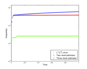
(a) Problem case (2)

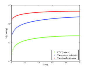
(b) Problem case (3)

Figure 1. The $L^{\infty}(0,t^{m},L^{2}(\varOmega))$-error, the two-level estimator ${\mathcal{E}}_{m}$ and the three-level estimator $\mathaccent 869{{\mathcal{E}}}_{m}.$

We exclude from the numerical experiments the coarsening error estimator ${\mathcal{E}}_{N}^{C}$ that vanishes as well as the terms corresponding to the approximation of data $u^{0}$ and $f$ which clearly are of optimal order and thus do not contain interesting information for our purposes. Moreover, we compute the total estimators ${\mathcal{E}}_{m}$ and $\mathaccent 869{{\mathcal{E}}}_{m},$ which correspond to two time-level reconstruction and three time-level reconstruction, respectively, defined as follows

(5.1) $${\mathcal{E}}_{m}:={\mathcal{E}}_{m}^{T,1}(w_{n})+{\mathcal{E}}_{m}^{T,2}+{\mathcal{E}}_{m}^{S,1}(w_{n})+{\mathcal{E}}_{m}^{S,2}+{\mathcal{E}}_{m}^{\text{ell}}+{\mathcal{E}}_{m}^{\text{rec}}(w_{n}),\quad 1\leq m\leq N,$$

and

$$\mathaccent 869{{\mathcal{E}}}_{m}:={\mathcal{E}}_{m}^{T,1}(\mathaccent 869{w}_{n})+{\mathcal{E}}_{m}^{T,2}+{\mathcal{E}}_{m}^{T,3}+{\mathcal{E}}_{m}^{S,1}(\mathaccent 869{w}_{n})+{\mathcal{E}}_{m}^{S,2}+{\mathcal{E}}_{m}^{\text{ell}}+{\mathcal{E}}_{m}^{\text{rec}}(\mathaccent 869{w}_{n}),\quad 1\leq m\leq N.$$

Then, the corresponding effectivity indices are defined as

$$EI(t^{m}):=\frac{{\mathcal{E}}_{m}}{\max_{0\leq n\leq m}\|e^{n}\|}\quad\text{and}\quad\tilde{EI}(t^{m}):=\frac{\tilde{\mathcal{E}}_{m}}{\max_{0\leq n\leq m}\|e^{n}\|}\,,\quad 1\leq m\leq N.$$

For all quantities of interest we look at their experimental order of convergence (EOC). The EOC is defined as follows: for a given finite sequence of successive runs (indexed by $i$), the EOC of the corresponding sequence of quantities of interest $E(i)$ (error, estimator or part of an estimator), is itself a sequence defined by

$${\rm EOC}(E(i))=\frac{\log(E(i+1)/E(i))}{\log(h(i+1)/h(i))}\,,$$

where $h(i)$ denotes the mesh-size of the run $i.$ The values of EOC of a given quantity indicates its order.

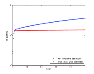
(a) Problem case (2)

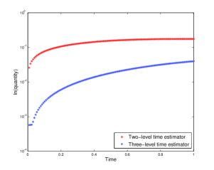
(b) Problem case (3)

Figure 2. The two-level time estimator ${\mathcal{E}}_{m}^{T,1}(w_{n})+{\mathcal{E}}_{m}^{T,2}+{\mathcal{E}}_{m}^{\text{rec}}(w_{n})$ and the three-level time estimator ${\mathcal{E}}_{m}^{T,1}(\mathaccent 869{w}_{n})+{\mathcal{E}}_{m}^{T,2}+{\mathcal{E}}_{m}^{T,3}+{\mathcal{E}}_{m}^{\text{rec}}(\mathaccent 869{w}_{n}).$

(a) Problem case (2)

(b) Problem case (3)

Figure 3. The two-level space estimator ${\mathcal{E}}_{m}^{S,1}(w_{n})+{\mathcal{E}}_{m}^{S,2}+{\mathcal{E}}_{m}^{\text{ell}}$ and the three-level space estimator ${\mathcal{E}}_{m}^{S,1}(\mathaccent 869{w}_{n})+{\mathcal{E}}_{m}^{S,2}+{\mathcal{E}}_{m}^{\text{ell}}.$

Errors

h = k	$\max_{n}\|e^{n}\|$	EOC	$e_{\rm total}(t^{N})$	EOC	${\mathcal{E}}_{N}$	$EI(t^{N})$	$\mathaccent 869{{\mathcal{E}}}_{N}$	$\mathaccent 869{EI}(t^{N})$
1.2500e-01	1.4481e-03		3.7925e-02		3.6810e-01	254	4.9986e-01	345
6.2500e-02	3.4561e-04	2.04	1.8534e-02	1.03	8.6375e-02	249	1.2473e-01	360
3.1250e-02	8.4256e-05	2.02	9.1731e-03	1.01	2.0828e-02	247	3.1030e-02	368
1.5625e-02	2.0821e-05	2.01	4.5645e-03	1.00	4.7780e-03	229	7.7309e-03	371
7.8125e-03	5.1718e-06	2.00	2.2769e-03	1.00	1.1813e-03	228	1.9289e-03	372

Table 1. Problem case (1): the $L^{\infty}(0,1;L^{2}(\varOmega))$-error, the total error $e_{\rm total}(t^{N}),$ and the corresponding EOCs, the two- and three-level estimators ${\mathcal{E}}_{N}$ and $\mathaccent 869{{\mathcal{E}}}_{N},$ respectively, and the corresponding effectivity indices $EI(t^{N})$ and $\mathaccent 869{EI}(t^{N})$.

Reconstruction Error Estimators

h = k	$\mathcal{E}_{N}^{\emph{ell}}$	EOC	$\mathcal{E}_{N}^{\emph{rec}}(w_{n})$	EOC	$\mathcal{E}_{N}^{\emph{rec}}(\mathaccent 869{w}_{n})$	EOC
1.2500e-01	2.2702e-02		3.2184e-02		9.9205e-03
6.2500e-02	5.6786e-03	1.99	7.7765e-03	2.03	2.4275e-03	2.02
3.1250e-02	1.4198e-03	2.00	1.9227e-03	2.01	6.0352e-04	2.00
1.5625e-02	3.5497e-04	2.00	4.7951e-04	2.00	1.5066e-04	2.00
7.8125e-03	8.8741e-05	2.00	1.1979e-04	2.00	3.7654e-05	2.00

Table 2. Problem case (1): the elliptic reconstruction estimator $\mathcal{E}_{N}^{\text{ell}},$ the time reconstruction estimators $\mathcal{E}_{N}^{\text{rec}}(w_{n}),\mathcal{E}_{N}^{\text{rec}}(\mathaccent 869{w}_{n})$ and the corresponding EOCs.

Since the finite element spaces consist of linear Lagrange elements and the Crank–Nicolson method is second-order accurate, the error in $L^{\infty}(0,T;L^{2}(\varOmega))$ norm is $O(k^{2}+h^{2})$. The main conclusion of this paragraph is that all error estimators, in both cases of time reconstruction, decrease with at least second order with respect to time and spatial variable, Tables 1-4.

Time Estimators

h = k	$\mathcal{E}_{m}^{T,1}(w_{n})$	EOC	${\mathcal{E}}_{m}^{T,1}(\mathaccent 869{w}_{n})$	EOC	$\mathcal{E}_{m}^{T,2}$	EOC	${\mathcal{E}}_{m}^{T,3}$	EOC
1.2500e-01	8.5528e-02		2.6086e-02		1.5603e-01		2.3606e-01
6.2500e-02	1.9581e-02	2.09	6.0501e-03	2.07	3.9203e-02	1.99	6.0174e-02	1.98
3.1250e-02	4.6603e-03	2.05	1.4486e-03	2.04	9.7796e-03	2.00	1.5116e-02	1.99
1.5625e-02	1.1340e-03	2.02	3.5392e-04	2.02	2.4396e-03	2.00	3.7834e-03	1.99
7.8125e-03	2.7935e-04	2.01	8.7434e-05	2.01	6.0908e-04	2.00	9.4614e-04	2.00

Table 3. Problem case (1): the time estimators $\mathcal{E}_{N}^{T,1}(w_{n}),{\mathcal{E}}_{N}^{T,1}(\mathaccent 869{w}_{n}),\mathcal{E}_{N}^{T,2},{\mathcal{E}}_{N}^{T,3}$ and the corresponding EOCs.

Space Estimators

h = k	$\mathcal{E}_{N}^{S,1}(w_{n})$	EOC	${\mathcal{E}}_{N}^{S,1}(\mathaccent 869{w}_{n})$	EOC	$\mathcal{E}_{N}^{S,2}$	EOC
1.2500e-01	3.1258e-02		8.6889e-03		4.0374e-02
6.2500e-02	4.0411e-03	2.78	1.1079e-03	2.80	1.0095e-02	2.00
3.1250e-02	5.2213e-04	2.78	1.3917e-04	2.82	2.5239e-03	2.00
1.5625e-02	6.7829e-05	2.77	1.7417e-05	2.82	6.3099e-04	2.00
7.8125e-03	8.7779e-06	2.77	2.1778e-06	2.82	1.5775e-04	2.00

Table 4. Problem case (1): the space estimators $\mathcal{E}_{N}^{S,1}(w_{n}),\mathcal{E}_{N}^{S,1}(\mathaccent 869{w}_{n}),\mathcal{E}_{N}^{S,2}$ and the corresponding EOCs.

References

• [1] G. Akrivis, C. Makridakis, and R. H. Nochetto. A posteriori error estimates for the Crank–Nicolson method for parabolic equations. Math. Comp., 75:511–531, 2006.
• [2] E. Bänsch, F. Karakatsani, and C. Makridakis. A posteriori error control for fully discrete Crank–Nicolson schemes. SIAM J. Numer. Anal., 6:2845–2872, 2012.
• [3] E. Bänsch, F. Karakatsani, and C. Makridakis. The effect of mesh modification in time on the error control of fully discrete approximations for parabolic equations. Appl. Numer. Math., 67:35–63, 2013.
• [4] M. Bristeau, R. Glowinski, and J. Periaux. Numerical methods for Navier–Stokes equations. applications to the simulation of compressible and incompressible viscous flows. Computer Physics Reports, 6:73–187, 1987.
• [5] K. Eriksson and C. Johnson. Adaptive finite element methods for parabolic problems. I. A linear model problem. SIAM J. Numer. Anal., 28(1):43–77, 1991.
• [6] K. Eriksson and C. Johnson. Adaptive finite element methods for parabolic problems. IV. Nonlinear problems. SIAM J. Numer. Anal., 32(6):1729–1749, 1995.
• [7] R. Glowinski. Viscous flow simulations by finite element methods and related numerical techniques. In E. Murman and S. Abarbanel, editors, Progress in Supercomputing in Computational Fluid Dynamics, pages 173–210. Birkhäuser, Boston, 1985.
• [8] R. Glowinski. Splitting methods for the numerical solution of the incompressible Navier–Stokes equations. In A. D. A.V. Balakrishman and J. Lions, editors, Vistas in Applied Mathematics, pages 57–95. Optimization Software, New York, 1986.
• [9] R. Glowinski. Finite element methods for incompressible viscous flow. In Handbook of numerical analysis, Vol. IX. North-Holland, Amsterdam, 2003.
• [10] C. Johnson, Y. Y. Nie, and V. Thomée. An a posteriori error estimate and adaptive timestep control for a backward Euler discretization of a parabolic problem. SIAM J. Numer. Anal., 27(2):277–291, 1990.
• [11] F. Karakatsani. A posteriori error estimates for the fractional-step $\vartheta$-scheme for linear parabolic equations. IMA J. Numer. Anal., 32(1):141–162, 2012.
• [12] O. Lakkis and C. Makridakis. Elliptic reconstruction and a posteriori error estimates for fully discrete linear parabolic problems. Math. Comp., 75(256):1627–1658, 2006.
• [13] A. Lozinski, M. Picasso, and V. Prachittham. An anisotropic error estimator for the Crank-Nicolson scheme. SIAM J. Sci. Comp, 31(4):2757–2783, 2009.
• [14] C. Makridakis and R. H. Nochetto. Elliptic reconstruction and a posteriori error estimates for parabolic problems. SIAM J. Numer. Anal., 41(4):1585–1594, 2003.
• [15] D. Meidner and T. Richter. Goal-oriented error estimation for the fractional step theta scheme. Computational Methods in Applied Mathematics, 2014.
• [16] S. Müller, A. Prohl, R. Rannacher, and S. Turek. Implicit time-discretization of the nonstationary incompressible navier-stokes equations. In W. Hackbusch and G. Wittum, editors, Proc. Workshop. “Fast Solvers for Flow Problems”, pages 175–191, Kiel, Germany, Jan. 14-16 1994. Vieweg, Braunschweig.
• [17] S. Müller-Urbaniak. Eine Analyse des Zwischenschritt-$\theta$-Verfahrens zur Lösung der instationären Navier-Stokes-Gleichungen. PhD thesis, University of Heidelberg, 1993.
• [18] R. H. Nochetto, G. Savaré, and C. Verdi. A posteriori error estimates for variable time-step discretizations of nonlinear evolution equations. Comm. Pure Appl. Math., 53(5):525–589, 2000.
• [19] V. Prachittham. Space-time adaptive algorithms for parabolic problems: a posteriori error estimates and application to microfluidics. Ph. d. thesis, EPFL, Laussane, 2009.
• [20] R. Rannacher. Numerical analysis of nonstationary fluid flow (a survey). In V. Boffi and H. Neunzert, editors, Applications of Mathematics in Industry and Technology, pages 34–53. B.G. Teubner, Stuttgart, 1998.
• [21] A. Schmidt and K. Siebert. Design of adaptive finite element software: The finite element toolbox ALBERTA, volume 42 of Springer LNCSE Series. Springer-Verlag, Berlin, 2005.
• [22] L. R. Scott and S. Zhang. Finite element interpolation of nonsmooth functions satisfying boundary conditions. Math. Comp., 54(190):483–493, 1990.
• [23] V. Thomée. Galerkin finite element methods for parabolic problems. Springer-Verlag, Berlin, 1997.
• [24] R. Verfürth. A posteriori error estimates for finite element discretizations of the heat equation. Calcolo, 40:195–212, 2003.
• [25] M. F. Wheeler. A priori ${L}_{2}$ error estimates for Galerkin approximations to parabolic partial differential equations. SIAM J. Numer. Anal., 10:723–759, 1973.