Global ab initio potential energy surface for the O${}_{2}(^{3}\Sigma^{-}_{g})$ + N${}_{2}(^{1}\Sigma^{+}_{g})$ interaction. Applications to the collisional, spectroscopic, and thermodynamic properties of the complex

Abstract

A detailed characterization of the interaction between the most abundant molecules in air is important for the understanding of a variety of phenomena in atmospherical science. A completely ab initio global potential energy surface (PES) for the O${}_{2}(^{3}\Sigma^{-}_{g})$ + N${}_{2}(^{1}\Sigma^{+}_{g})$ interaction is reported for the first time. It has been obtained with the symmetry-adapted perturbation theory utilizing a density functional description of monomers [SAPT(DFT)] extended to treat the interaction involving high-spin open-shell complexes. The computed interaction energies of the complex are in a good agreement with those obtained by using the spin-restricted coupled cluster methodology with singles, doubles and noniterative triple excitations [RCCSD(T)]. A spherical harmonics expansion containing a large number of terms due to the anisotropy of the interaction has been built from the ab initio data. The radial coefficients of the expansion are matched in the long range with the analytical functions based on the recent ab initio calculations of the electric properties of the monomers [M. Bartolomei et al., J. Comp. Chem., 32, 279 (2011)]. The PES is tested against the second virial coefficient $B(T)$ data and the integral cross sections measured with rotationally hot effusive beams, leading in both cases to a very good agreement. The first bound states of the complex have been computed and relevant spectroscopic features of the interacting complex are reported. A comparison with a previous experimentally derived PES is also provided.

I Introduction

Simple molecular gases interact in our atmosphere and the outer space through weak intermolecular forces giving rise to many different processes that roughly speaking are characterized by the energy transfer and momentaneous rearrangements of their isolated charge distributions. It is, therefore, of a paramount interest an accurate description of these weak interactions and properties that appear as a consequence. Among these simple molecular species, O₂ and N₂ are central because of their abundance in our atmosphere, and their importance for life.

Another important consequence of the weak intermolecular forces is the existence of weakly bound complexes, mainly dimers. In some cases as, in the O₂ dimer, its existence was already suggested as early as 1924 when LewisLewis (1924) proposed the existence of a strong bound between two oxygen molecules. In search of such a dimer Welsh et. alCrawford et al. (1949) found much stronger and universal bands, which are known as Collision-Induced AbsorptionFrommhold (1994) (CIA). Both the dimeric complex and CIA are close and related phenomena that are important not only for spectroscopic purposesAbel and Frommhold (2013), but for the energy transfer rates and other observables that are key ingredients in the atmospheric modelingKlemperer and Vaida (2006) and many other areas in which the delicate balance between radiative and non-radiative processes is neccesary to reach an acceptable agreement with observation.

Since the importance of the previously mentioned effects are intimately related to the gas density, the knowledge of an accurate potential energy surface (PES) that could describe short and long-range behavior at once becomes evident.

For the oxygen dimer, we have recently succeeded in producing a global potential energy surface with ab initio calculations at a high level of theory. In particular, for the quintet state multiplicity a restricted coupled-cluster theory with singlet, doubles, and perturbative triple excitations [RCCSD(T)] was successfully usedBartolomei et al. (2008a) to compute this PES. This state is well represented by a single configuration while the singlet and triplet states are inherently multiconfigurational and therefore the CCSD(T) cannot be applied. A scheme was proposedBartolomei et al. (2008b) to sort out this problem that was based on a difference procedure involving multireference electronic structure methods. The result is a global potential energy surfaceBartolomei et al. (2010) that yields excellent results as compared with all experimental data available and both for the short and long rangeBartolomei et al. (2011). In the case of the nitrogen dimer, although it is not an open-shell system it was not easy to accomplish an accurate description until recently. Currently, there are several ab initio PESGomez et al. (2007) that have been computed using Symmetry Adapted Perturbation Theory (SAPT)Jeziorski et al. (1994), and that have been very recently usedBussery-Honvault and Hartmann (2014) to study CIA for nitrogen.

The data for the heterodimer $N_{2}-O_{2}$ are scarcer, even though an accurate description of the interactions is of primordial relevance to interpret data from observation and remote sensing and atmospheric modeling. One of the few available PES is an experimentally derived potential energy surfaceAquilanti et al. (2003) (Perugia-PES, from now on), which was obtained from molecular beam experiments and gives an excellent answer when compared with available experimental data.

Here, we employ SAPT(DFT) to calculate for the first time an accurate ab initio PES that is further expanded in order to have a functional form ready to use in dynamical calculations. The performance of the newly computed PES is compared with previous ones as well as tested against experimental data. It should be stressed that the SAPT(DFT) approach is particularly well suited for the calculations of global potential energy surfaces for weakly bound complexes. As shown in Ref. Zuchowski et al. (2008) the accuracy of the SAPT(DFT) results is often comparable to RCCSD(T), while the computational cost is much lower.

The paper is organized as follows. Section II gives the details of the PES calculations, including the angular expansion and the long-range behavior. In Section III we discuss the topography of the potential energy surface and compare the computed second virial coefficients and integral cross sections with the available experimental data. In Section IV we report calculations of the bound rovibrational levels. Finally, in Section V we conclude our paper.

II The O₂-N₂ PES: calculations

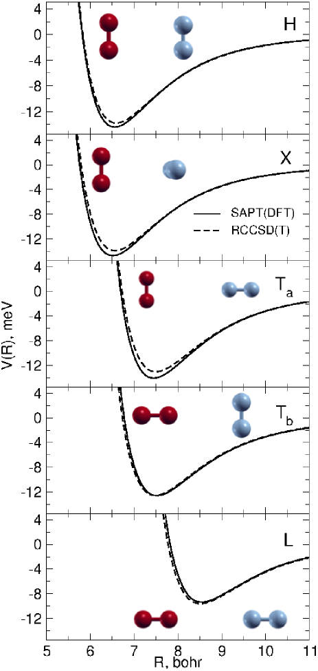
Figure 1: Comparison between SAPT(DFT) and RCCSD(T) intermolecular potentials at five limiting orientations of O₂-N₂ as obtained by using the aug-cc-pVTZ plus bond function basis set (see text). The different arrangements are depicted in the insets, where O and N atoms are symbolized by red and light blue balls, respectively.

Diatom-diatom Jacobi vectors, ${\bf r}_{a}$, ${\bf r}_{b}$ and ${\bf R}$, are used, where ${\bf r}_{a}$ and ${\bf r}_{b}$ are the interatomic vectors of O₂ and N₂, respectively, and ${\bf R}$ is the vector joining the centers of mass of the diatoms. Thus, the six internal coordinates determining the O₂-N₂ PES are the distances $R$, $r_{a}$, and $r_{b}$, and $\theta_{a}$, $\theta_{b}$, and $\phi$, the angles formed by ${\bf R}$ and ${\bf r}_{a}$, ${\bf R}$ and ${\bf r}_{b}$, and the torsional angle, respectively. In the PES reported here, the intramolecular distances have been fixed at the O₂ and N₂ equilibrium distances, $r_{a}$= 2.28 and $r_{b}$= 2.08 bohr, respectively, so that we describe the interaction between the diatoms in their ground vibrational states.

As done previouslyBartolomei et al. (2008a); Bartolomei et al. (2010) we have considered the geometries generated from 9 Gauss-Legendre quadrature points in the $-1\leq cos\theta_{a},cos\theta_{b}\leq 1$ range and from 5 Gauss-Chebyshev points for $0\leq\phi\leq\pi$. An initial range in the torsional angle from [0:$2\pi$] has been reduced to [0:$\pi$] by use of the permutation-inversion symmetry of this systemvan der Avoird and Brocks (1987), which also allows us to reduce the initial 9$\times$9$\times$5 grid to a 5$\times$5$\times$5 grid ($-1\leq cos\theta_{a},cos\theta_{b}\leq 0$). If we further consider the following equivalences due to symmetry $(\theta_{a},\pi/2,\phi)\equiv(\theta_{a},\pi/2,\pi-\phi)$ and $(\pi/2,\theta_{b},\phi)\equiv(\pi/2,\theta_{b},\pi-\phi)$, we are finally left with 107 “irreducible” geometries. For each angular arrangement, 18 points in the intermolecular coordinate $R$, ranging from 16.0 to 5.0 bohr, were considered.

II.1 SAPT(DFT) ab initio calculations

Table 1: Energies (in meV) for five limiting configurations at intermolecular distances close to the minima (in parenthesis, in bohr), as obtained from SAPT(DFT) with aug-cc-pVTZ and aug-cc-pVQZ basis sets plus bond functions (the same in both cases, see text).

	H (6.5)	X (6.5)	Ta (7.5)	Tb (7.5)	L (8.5)
VTZ	14.344	14.685	14.004	12.580	9.324
VQZ	14.549	14.909	14.104	12.723	9.322

Since the O₂ and N₂ monomers have electronic spins $S_{a}=1$ and $S_{b}=0$, respectively, the intermolecular potential does not depend on the spin couplings between the monomers and therefore accurate single reference approaches, such as SAPT(DFT) and spin-restricted RCCSD(T), can be applied. The SAPT(DFT) calculations were performed using the methodology of Ref. Zuchowski et al. (2008) which is suitable to obtain the interactions in high-spin dimers formed by open-shell monomers. The aug-cc-pVTZ and aug-cc-pVQZ basis setsKendall et al. (1992), both supplemented by the bond function set [3s3p2d1f] developed by TaoTao and Pan (1992) and placed in the middle of the intermolecular distance, have been used in the calculations. The monomer DFT calculations employed the PBE0 hybrid functionalAdamo and Barone (1999) and were done using the DALTONDal (2005) program. We applied the Fermi-Amaldi-Tozer-Handy asymptotic correctionFermi and Amaldi (1934); Tozer and Handy (1998) with the ionization potentials of 0.479 and 0.613 a.u.Żuchowski (2008) (for $\alpha$ and $\beta$ electrons, respectively) for O₂ and 0.5726 a.u.NIS for N₂. The SAPT(DFT) calculations used the open-shell SAPT(DFT) program of the SAPT2008 code Bukowski et al. (2008).

First, we have tested the basis set saturation and performances for some limiting configurations of the interacting complex: linear ($D_{\infty h}$), T-shaped ($C_{2v}$), rectangular ($D_{2h}$) and crossed ($D_{2d}$) arrangement, in the following, referred to as L, T, H and X, respectively. We distinguish two T-shaped orientations: T_a, where the O₂ intramolecular vector ${\bf r}_{a}$ is perpendicular to ${\bf R}$, and T_b, where N₂ is the diatom oriented perpendicularly to the intermolecular vector. Results are reported in Table 1. As can be noticed both sets provide almost identical results: the largest differences, corresponding to H and X configurations, are within 1 %. The analysis was extended to other intermolecular distances and it was found that the discrepancies between both basis sets remain of the same order of magnitude. We regard these deviations as acceptable, bearing in mind that for a single geometry on a single processor the aug-cc-pVTZ calculations are three times faster than those employing the larger basis set.

In order to further check the performance of the SAPT(DFT) results, supermolecular spin-restricted RCCSD(T)/aug-cc-pVTZ (plus bond functions) calculations have been performed for the same limiting configurations. The counterpoise methodBoys and Bernardi (1970); van Lenthe et al. (1987) was applied to correct for the basis set superposition error and the calculations were carried out with the Molpro2006.1 packageWerner et al. (2006). The comparison between the interaction energies obtained from the two different levels of theory are shown in Fig. 1. It can be noticed that SAPT(DFT) curves are somewhat more attractive in the well region for the most attractive configurations (H, X and T_a), while they are slightly more repulsive for the remaining arrangements (T_b and L). Overall the agreement can be termed as good since discrepancies are in general within 5 %. It is noteworthy to stress the saving in computing time provided by the SAPT(DFT) methodology. In fact we have estimated that for a single point/single CPU, RCCSD(T) calculations would be about six times slower than equivalent SAPT(DFT) ones if no symmetry is used (as it is for most of the geometrical arrangements).

Supported by the above mentioned tests we decided to choose the SAPT(DFT) methodology with the aug-cc-pVTZ basis supplemented with the [3s3p2d1f] set of bond functions for all the geometries needed to obtain a complete and reliable representation of the O₂-N₂ PES.

II.2 Spherical harmonics expansion

Table 2: Comparison of ab initio energies with those resulting from the spherical harmonic expansion of Eq. 1 using the set of 39 radial coefficients detailed in the text, for several orientations and intermolecular distances.

Geometry
$\theta_{a}$	$\theta_{b}$	$\phi$	$R$	$V_{abinitio}$	$V_{expanded}$	%
(degrees)			(bohr)	(meV)	(meV)
			5.25	71.30	71.63	0.46
H			5.50	28.10	28.08	0.07
90	90	0	6.25	-12.77	-12.84	0.55
			6.50	-14.34	-14.37	0.66
			7.00	-12.75	-12.75	0.21
			12.00	-0.513	-0.513	0.00
			14.00	-0.192	-0.192	0.00
			5.25	57.20	55.25	3.41
X			5.50	20.64	20.02	3.00
90	90	90	6.25	-13.59	-13.50	0.66
			6.50	-14.69	-14.63	0.41
			7.00	-12.80	-12.78	0.16
			12.00	-0.546	-0.546	0.00
			14.00	-0.209	-0.209	0.00
			5.25	577.57	577.84	0.05
Ta			5.50	341.08	340.70	0.11
90	0	0	7.25	-13.52	-13.52	0.00
			7.50	-14.00	-14.01	0.07
			8.00	-11.85	-11.85	0.00
			12.00	-0.954	-0.954	0.00
			14.00	-0.351	-0.351	0.00
			5.25	661.64	660.63	0.15
Tb			5.50	389.72	388.71	0.26
0	90	0	7.25	-11.57	-11.56	0.09
			7.50	-12.58	-12.57	0.08
			8.00	-11.01	-11.00	0.09
			12.00	-0.928	-0.928	0.00
			14.00	-0.350	-0.350	0.00
			5.25	3332.44	3344.74	0.37
L			5.50	2381.61	2384.07	0.10
0	0	0	8.25	-8.35	-8.33	0.24
			8.50	-9.32	-9.31	0.11
			9.00	-8.20	-8.21	0.12
			12.00	-1.129	-1.128	0.09
			14.00	-0.361	-0.361	0.00
			5.25	626.06	626.54	0.08
S45			5.50	386.29	386.37	0.02
45	45	0	7.25	-9.40	-9.38	0.21
			7.50	-11.40	-11.40	0.00
			8.00	-10.84	-10.84	0.00
			12.00	-0.945	-0.946	0.11
			14.00	-0.349	-0.349	0.00

The interaction potential $V$ is written using a spherical harmonics expansion asWormer and van der Avoird (1984):

$$V(R,\theta_{a},\theta_{b},\phi)\,=\,(4\pi)^{3/2}\,\sum_{l_{a},l_{b},l}\,f^{l_{a}l_{b}l}(R)\,A_{l_{a}l_{b}l}(\theta_{a},\theta_{b},\phi),$$ (1)

with

$$A_{l_{a}l_{b}l}(\theta_{a},\theta_{b},\phi)\, = \,\left(\frac{2l+1}{4\pi}\right)^{1/2}\,\sum_{m}\,\left(\begin{array}[]{rrr}l_{a}&l_{b}&l\\ m&-m&0\end{array}\right)$$ (5)

$$Y_{l_{a},m}(\theta_{a},0)\,Y_{l_{b},-m}(\theta_{b},\phi),$$

where $Y_{l_{a},m}$ and $Y_{l_{b},-m}$ are the normalized spherical harmonics that are coupled with a 3$j$ symbol, and $m$ runs from $-\min(l_{a},l_{b})$ to $\min(l_{a},l_{b})$. The radial coefficients $f^{l_{a}l_{b}l}(R)$ are computed by integrating $V$ over the angular variables:

$$f^{l_{a}l_{b}l}(R) = \pi^{1/2}\int_{-1}^{1}d(\cos\theta_{a})\int_{-1}^{1}d(\cos\theta_{b})\int_{0}^{2\pi}d\phi$$ (6)

$$V(R,\theta_{a},\theta_{b},\phi)A^{*}_{l_{a},l_{b},l}(\theta_{a},\theta_{b},\phi).$$

Integrals were carried out for each intermolecular distance $R$ by means of Gauss-Legendre (for $cos\theta_{a,b}$) and Gauss-Chebyshev (for $\phi$) quadraturesAbramovitz and Stegun (1972).

Due to the permutation-inversion symmetries of the complex, $l_{a}$, $l_{b}$, and $l$ integers must be even. In contrast with dimers of identical diatoms, however, $f^{l_{a}l_{b}l}$ and $f^{l_{b}l_{a}l}$ coefficients differ. From the set of quadrature points used in the present work, a series of 85 different radial coefficients arise, consisting in all the combinations $(l_{a}l_{b}l)$ where $l_{a},l_{b}$= 0, …, 8 and $\left|l_{a}-l_{b}\right|$ $\leq l\leq$ $l_{a}$+$l_{b}$. We have selected a subset of 39 radial coefficients for which the interaction potential is sufficiently well represented. It was built by discarding, for $l_{a}>4$ or $l_{b}>4$, all coefficients with $l\neq l_{a}+l_{b}$, except for $(l_{a}l_{b}l)$= (2 6 4), (2 6 6), (6 2 4) and (6 2 6). Root mean square (rms) relative and absolute errors of this expansion with respect to the ab initio energies (for all distances and quadrature points) are about 2 % and 0.55 meV, respectively.

A further indication of the quality of the spherical harmonics expansion is given in Table 2, where a comparison between ab initio interaction energies and those corresponding to the expansion is given for some selected geometries. This is an independent check of the accuracy of the expansion, since, except for the X geometry, none of these geometries correspond to the Gaussian quadrature points used to build the PES and then, they were computed independently. It can be seen that the comparison is satisfactory. The largest discrepancies are found at short intermolecular distances ($R\leq 5.5$ bohr) where the interaction becomes more anisotropic.

II.3 Long range behavior and matching procedure

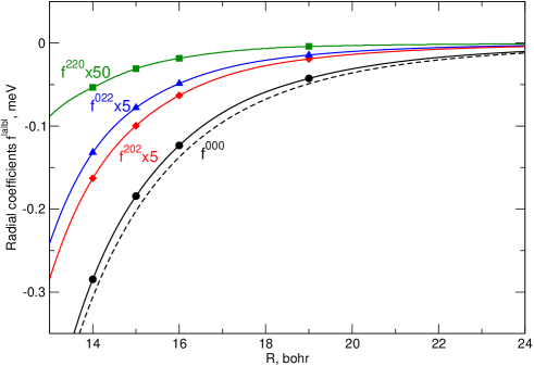
Figure 2: Behavior of the $f^{000}$, $f^{202}$, $f^{022}$ and $f^{220}$ radial coefficients at large intermolecular distances. Points at 14, 15 and 16 bohr are those resulting from the ab initio calculations, whereas Eq. (7) is used for $R$= 19 bohr. For $R<$ 19 bohr the curves are the result of cubic spline interpolation, while for larger $R$’s they are given by the analytical long range behavior of Eq. 7. The dashed line corresponds to the $f^{000}$ term of the experimentally derived PES of Ref.Aquilanti et al. (2003).

In this paragraph we present the asymptotic extension of the PES by using analytical expressions for the long range behavior. Following the Rayleigh-Schrödinger perturbation theory of intermolecular forces Cwiok et al. (1992) in the multipole approximation van der Avoird et al. (1980); Heijmen et al. (1996), the radial coefficients $f^{l_{a}l_{b}l}(R)$ of Eq. 1 can be written by a sum of electrostatic ($el$), dispersion ($d$) and induction ($i$) contributions:

$$f^{l_{a}l_{b}l}(R)=f^{l_{a}l_{b}l}_{el}(R)+f^{l_{a}l_{b}l}_{d}(R)+f^{l_{a}l_{b}l}_{i}(R),$$ (7)

where

$$f^{l_{a}l_{b}l}_{el}(R)=\delta_{l_{a}+l_{b},l}\left[\frac{(2l_{a}+2l_{b})!}{(2l_{a}+1)!(2l_{b}+1)!}\right]^{1/2}\frac{Q_{0}^{l_{a}}Q_{0}^{l_{b}}}{R^{l_{a}+l_{b}+1}},$$ (8)

and

$$f^{l_{a}l_{b}l}_{(d,i)}(R)=-\frac{1}{[(2l_{a}+1)(2l_{b}+1)(2l+1)]^{1/2}}\sum_{n}\frac{C_{n,(d,i)}^{l_{a}l_{b}l}}{R^{n}}.$$ (9)

Coefficients involved in Eqs. 8 and 9 have recently been obtained from high level ab initio calculationsBartolomei et al. (2011). Permanent electric multipole moments $Q_{0}^{l}$ ($l$=2,4,6,8) were taken from Tables III and IV of Ref.Bartolomei et al. (2011), and dispersion and induction coefficients $C_{n,(d,i)}^{l_{a}l_{b}l}$, (with $n$=6,8 and $n$=8, respectively, and $(l_{a}l_{b}l)$ up to (2 4 6) ), from Table VII of the same work.

The expression of Eq. 7 was used for distances $R\geq 19$ bohr. For shorter distances, $f^{(l_{a}l_{b}l)}(R)$ were calculated from cubic spline interpolation of the values $f_{i}^{(l_{a}l_{b}l)}$ obtained from the SAPT(DFT) calculations at the set of distances $R_{i},i=1,...,N$. An additional point $R_{N+1}$=19 bohr was included in that grid with a value given by Eq. 7. The analytical derivative of $f^{l_{a}l_{b}l}(R)$ at $R_{N+1}$ was used as a boundary condition for solving the interpolation equations, so that a smooth behavior of the radial term around $R_{N+1}$ is achieved. The procedure worked well, providing a good indication of the consistency between the SAPT(DFT) calculations and the computed electric properties of the molecular fragments. As an example, we show in Fig.2 the behavior of the first four coefficients around the matching region. In there the long range behavior of $f^{000}$ from the Perugia-PESAquilanti et al. (2003) is also reported.

III Results and discussion

III.1 The potential energy surface

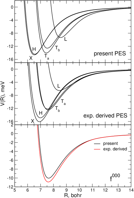
Figure 3: Comparison between present ab initio PES and the experimentally derived one from Ref. Aquilanti et al. (2003). Upper and intermediate panels: potential energy (in meV) profiles as functions of the intermolecular distance $R$ (in bohr) for selected geometries of the dimer. Lower panel: spherical average $f^{000}$ as a function of $R$.

Table 3: Equilibrium distances $R_{m}$ (in bohr) and well depths $D_{m}$ (in meV) of the O₂-N₂ PES at some selected orientations as well as the spherical average. Present results are compared with those of Perugia-PESAquilanti et al. (2003).

	Ref.Aquilanti et al. (2003)		This work
	$D_{m}$	$R_{m}$	$D_{m}$	$R_{m}$
H	14.89	6.99	14.41	6.56
X	16.08	6.92	14.63	6.52
Ta	12.17	7.54	14.05	7.44
Tb	12.45	7.58	12.58	7.52
L	6.52	8.47	9.33	8.54
S45	8.76	8.01	11.68	7.66
f000	10.90	7.60	10.04	7.62

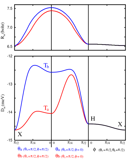
Figure 4: Low energy pathways of the present O₂-N₂ PES. As the relative orientation of the diatoms is varied as indicated in the abscissae labels, the associated equilibrium distances $R_{m}$ (upper panel) and well depths $D_{m}$ (lower panel) are displayed. Left panels: from the crossed X to T_a and T_b geometries; center panels: from the latter to the H configuration; right panels: from H to the X orientation.

In Fig. 3 and Table 3, we report the most prominent features of the present PES in comparison with those of the Perugia-PESAquilanti et al. (2003). Both intermolecular potentials are in a good qualitative agreement. For example, the crossed configuration (X) is the most stable geometry for both PESs, while a good match in the equilibrium distance and well depth of the spherically averaged interaction is observed. Nevertheless, some important differences can be found when going into details. In fact, present calculations give shorter equilibrium distances for the parallel (H) and the crossed (X) configurations, the curves being almost identical for these two orientations. Moreover, the ab initio well depth of the T_a geometry is larger than the T_b one, and it is very close to those of the most stable X and H arrangements. This is in contrast with the features of the T-shaped geometries of the Perugia-PESAquilanti et al. (2003) (see the intermediate panel of Fig. 3). In general, the present PES provides deeper potentials for the more repulsive geometries (T-shaped and collinear L), while for the most attractive ones (X and H), slightly shallower wells. In spite of this, we believe that the ab initio PES is more anisotropic since, at a given $R$, the interaction energy exhibits a stronger dependence with the angles than in the Perugia-PES case.

The ab initio spherically averaged radial term ($f^{000}$) is compared with that of Ref.Aquilanti et al. (2003) in the lower panel of Fig. 3. This test is meaningful because the latter was obtained from analyses of accurate integral cross section dataBrunetti et al. (1981). As can be seen, although present calculations slightly underestimate the experimentally derived interaction energy in the well and repulsive regions, the matching for the equilibrium distance, $R_{m}$, is very good (see Table 3). Differences in the interaction energy are less than 1 meV near the equilibrium distance and become almost negligible in the long range tail (see also Fig. 2).

More insight into the features of the O₂-N₂ interaction is gained from Fig. 4, where we show a few representative pathways joining the most stable configurations X, T_a, T_a, and H. First, it is worthwhile noticing the almost flat path between the H and X geometries, suggesting a free internal (torsional) rotation in the dimer. In addition, it can be seen that the paths connecting the T-shaped structures with the most stable H or X geometries involve very small barriers (except for the T_a-H path). This finding brings a picture of the O₂-N₂ dimer as a rather floppy cluster.

III.2 Integral cross sections

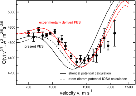
Figure 5: Total integral cross sections $Q(v)$ times $v^{2/5}$, for scattering of a rotationally hot O₂ effusive beam by N₂ target molecules as functions of the beam velocity, $v$. Present calculations are in solid and dashed black lines as obtained with a spherical average and an atom-diatom dynamical models, respectively (see text). Experimental data (filled circles with error bars) and related best fit calculations (in red) are from Refs. Brunetti et al. (1981); Aquilanti et al. (2003).

In order to assess the reliability of the present PES, we have tested it against available experimental data such as the total integral cross sections reported in Refs. Brunetti et al. (1981); Aquilanti et al. (2003) for the scattering of rotationally hot and near effusive O₂ beams. In these experiments, oxygen projectiles are at a high rotational temperature (about 10³ K) and collide with target N₂ molecules which are in the scattering chamber at low translational temperature. Under these conditions Brunetti et al. Brunetti et al. (1981) were able to resolve the glory structure which in turn can give valuable informationCappelletti et al. (2008); Bartolomei et al. (2008c); Thibault et al. (2009) on the intermolecular interaction involved. As explained before (see Ref. Aquilanti et al. (2003) and references therein), at low collision velocities, the colliders mainly probe the isotropic component of the interaction, while the anisotropy plays an increasing role at intermediate and high velocities.

Accordingly, we have computed total cross sections $Q(v)$ using two different schemes. In one case, we have used just the first term of the expansion of Eq. 1, $f^{000}$, which represents the spherical average of the PES. In a second approach, we have used the potential energy surface in an atom-diatom limit, corresponding to the interaction averaged over the orientation of the O₂ projectileAquilanti et al. (2003). In the latter case, the surface reduces to the sum of just five terms arising in Eq. 1 when the $(l_{a},l_{b},l)$= (0 $l_{b}$ $l_{b}$) constraint is imposed ($l_{b}$=0,2,4,6,8) and the calculations where performed using the infinite-order-sudden (IOS) approximation. In both approaches the phase shifts have been evaluated within the JWKB approximation. The center-of-mass cross sections are then convoluted over the relative velocity distribution and transformed to the laboratory reference frame. More technical details can be found in Ref. Cappelletti et al. (2002) and references therein.

In Fig. 5 we report the cross sections obtained within the two proposed schemes and using the ab initio PESs, in comparison with those obtained using the experimentally derived PES as well as the experimental resultsAquilanti et al. (2003). An overall good agreement is noticed. The average value of the ab initio cross sections is just a few percents lower ($<$ 2 %) than the best experimental fit, with the glory pattern slightly shifted towards lower velocities. The IOS results with the effective atom-diatom potential better describe the observed glory oscillations than the isotropic potential. It is generally admitted that the average values of the cross sections contain information about the long-range attractionSchiff (1956); Pirani and Vecchiocattivi (1982). In this context and for the velocities probed experimentally, the “long range region” corresponds to intermolecular distances of about 11-14 bohrAquilanti et al. (1998); Pérez-Ríos et al. (2009) where a good matching between the present and the experimentally derived PESs was already noted (see Figs. 2 and 3). On the other hand, it is also well known that the glory structures of the cross sections provide information on the potential well areaBernstein and O’Brien (1965, 1967). In addition to this, it has been pointed out recentlyPérez-Ríos et al. (2012) that anisotropy can also influence the velocity positions of the glory extrema in molecule-molecule scattering. In fact, it can be seen in Fig.5 that the glory extrema shift to higher velocities when one moves from the atom-atom to the atom-diatom approximation. Thus, we expect that the full molecule-molecule scattering calculation would shift the glory pattern towards even higher velocities (as found for O₂-O₂Pérez-Ríos et al. (2012)), eventually bringing theoretical results to a closer agreement with the measurements.

III.3 Second virial coefficients

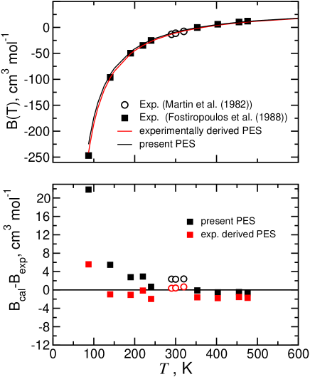
Figure 6: Upper panel: Second virial coefficients $B(T)$ as a function of temperature. Present calculations are compared with those obtained with the Perugia-PESAquilanti et al. (2003) as well as with the experimental data of Martin et al Martin et al. (1982) and Fostiropoulos et al Fostiropoulos et al. (1988). Lower panel: Deviations between experimental and calculated $B(T)$’s.

Table 4: Calculated and measured values of the second virial coefficient $B(T)$ (cm³ mol^-1) as a function of temperature (in K). Values corresponding to the contribution given by the spherical component of the interaction are shown in parentheses.

$T$ (K)	PES Ref.Aquilanti et al. (2003)		This work		Experimental
87.2	-241.4	(-206.1)	-225.2	(-172.1)	-247.0$\pm 7$a
90.0	-227.1	(-194.2)	-212.0	(-162.1)
100.0	-185.7	(-159.3)	-173.5	(-132.5)
110.0	-155.0	(-133.0 )	-144.9	(-110.0)
125.0	-121.4	(-103.8)	-113.5	(-84.9)
140.0	-97.3	(-82.7)	-90.8	(-66.6)	-96.3$\pm 5$a
190.0	-50.7	(-41.2)	-46.8	(-30.2)	-49.6$\pm 4$a
220.0	-34.9	(-27.0)	-31.9	(-17.6)	-34.8$\pm 3$a
240.0	-27.1	(-19.8)	-24.4	(-11.3)	-25.1$\pm 2$a
290.0	-12.9	(-6.9)	-10.9	(0.1)	-13.3b
300.0	-10.9	(-5.0)	-8.9	(1.9)	-11.2b
320.0	-6.9	(-1.5)	-5.2	(5.0)	-7.6b
353.0	-1.7	(3.3)	-0.2	(9.3)	-0.1$\pm 2$a
403.0	4.3	(8.9)	5.6	(14.2)	6.1$\pm 3$a
455.0	8.9	(13.1)	10.0	(18.0)	10.5$\pm 3$a
476.0	10.5	(14.5)	11.5	(19.2)	12.2$\pm 3$a
500.0	12.1	(16.0)	13.0	(20.5)
600.0	17.0	(20.5)	17.8	(24.5)
700.0	20.3	(23.5)	21.0	(27.2)
800.0	22.6	(25.6)	23.2	(29.0)
900.0	24.2	(27.0)	24.8	(30.2)
1000.0	25.4	(28.1)	26.0	(31.2)

^a Fostiropoulos et alFostiropoulos et al. (1988)
^b Martin et al Martin et al. (1982)

A further check of the quality of the present PES is carried out through the computation of the second virial coefficient $B(T)$ as a function of the temperature $T$. To this end we apply the semiclassical theory based on the expressions for two linear molecules presented by PackPack (1983) which include the first quantum correction due to the relative translational and rotational motions, including Coriolis coupling.

In Table 4 and in Fig. 6 (upper panel), the calculated values of $B(T)$ are compared with the experimental data of Refs.Martin et al. (1982); Fostiropoulos et al. (1988), together with those corresponding to the Perugia-PESAquilanti et al. (2003). A more detailed analysis of the deviations of the calculations with respect to the measurements is given in the lower panel of Fig. 6. It can be seen that, except for the results at $T$= 87.2 K, the comparison with the experimental data of Ref.Fostiropoulos et al. (1988) is very good and almost perfect around and above the Boyle temperature ($T\sim$ 353 K). In fact, the ab initio PES works better in the high temperature region than the experimentally derived PES. These results indicate that the present PES is well characterized, especially in the repulsive region.

The role of the anisotropy can be inferred from the comparison of $B(T)$ obtained using the full PES with a calculation where the anisotropy is neglected just by retaining the isotropic component of the interaction. The results of the latter calculations are shown in parentheses in Table 4. It can be noticed that there are significant differences between the two approaches and that this discrepancy increases as temperature decreases. Interestingly, the isotropic approximation as obtained using the ab initio PES leads to less negative and more positive $B(T)$ at low and high temperatures, respectively, if compared with the results from the experimentally derived PES. This is due to the less attractive character of the isotropic component for the ab initio PES as already discussed above (see also Fig.3). However, the contribution of the anisotropy is more important in the ab initio than in the experimentally derived PES, which in turn compensates the isotropic contribution and globally leads to a good agreement with the experimental $B(T)$.

Since second virial coefficient measurements for gas mixtures are in general less accurate than those for pure gases Eubank and Hall (1990) we find useful to provide data for temperatures higher than those considered in the experiments, as shown in Table 4. Based on the previous analysis, we believe that present results for the second virial coefficients $B(T)$ are the best theoretical estimates to date for temperatures higher than 353 K and, for $T>$ 500 K, they should be taken as the reference data.

IV Bound state calculations

Table 5: Energies (in meV and cm^-1) of the lowest rotationless ($J$=0) states of ¹⁶O₂-¹⁴N₂. The parity of $j_{a}$ (O₂), $j_{b}$ (N₂) and $l$ in the wave function expansion is indicated, together with the parity of the total eigenfunctions (including the electronic part) with respect to the operations of the $G_{8}$ group, and their symmetry (as in Table A-22, page 393 of Ref.Bunker (1979)). Allowed states are given in boldface.

Level	$E$(meV)	$E$(cm-1)		$j_{a}\;j_{b}\;l$		$P_{12}\;P_{34}\;E^{*}$		Sym
0	-10.32	-83.28		$e\;e\;e$		$-\;+\;+$		B${}_{2}^{\prime\prime}$
1	-9.81	-79.11		$o\;o\;o$		$+\;-\;-$		B${}_{1}^{\prime}$
2	-9.72	-78.37		$o\;o\;e$		$+\;-\;+$		B${}_{2}^{\prime}$
3	-9.39	-75.78		$e\;o\;o$		$-\;-\;+$		A${}_{1}^{\prime\prime}$
4	-9.16	-73.89		$o\;e\;o$		$+\;+\;+$		A${}_{1}^{\prime}$
5	-8.75	-70.59		$e\;e\;e$		$-\;+\;+$		B${}_{2}^{\prime\prime}$
6	-8.65	-69.79		$e\;e\;e$		$-\;+\;+$		B${}_{2}^{\prime\prime}$
7	-8.33	-67.23		$o\;e\;e$		$+\;+\;-$		A${}_{2}^{\prime}$
8	-8.32	-67.09		$o\;e\;o$		$+\;+\;+$		A${}_{1}^{\prime}$
9	-8.25	-66.53		$e\;e\;o$		$-\;+\;-$		B${}_{1}^{\prime\prime}$
10	-8.24	-66.46		$e\;e\;e$		$-\;+\;+$		B${}_{2}^{\prime\prime}$
11	-8.19	-66.08		$e\;o\;o$		$-\;-\;+$		A${}_{1}^{\prime\prime}$
12	-8.14	-65.68		$e\;o\;e$		$-\;-\;-$		A${}_{2}^{\prime\prime}$

In this section, we report energies and geometries of the lowest bound states of O₂-N₂. Since the intramolecular distances have been fixed in the ab initio PES, the diatoms O₂ and N₂ are treated as rigid rotors wihin the present approach. The Hamiltonian describing the nuclear motion writes -using the previously defined diatom-diatom Jacobi coordinates in a space-fixed (SF) frame as Green (1975); van der Avoird et al. (1994)

$$H = -\frac{1}{2\mu R}\frac{\partial^{2}}{\partial R^{2}}R+\frac{{\bf\hat{\ell}}^{2}}{2\mu R^{2}}+B_{a}\,{\bf{\hat{j}_{a}}}^{2}+B_{b}\,{\bf{\hat{j}_{b}}}^{2}+V,$$ (10)

where atomic units are used ($\hbar=1$), $\mu$ is the reduced mass of the complex, $V$ is the PES, $B_{a,b}$ are the rotational constants of O₂ and N₂, respectively, and ${\bf\hat{\ell}}$, ${\bf{\hat{j}_{a}}}$ and ${\bf{\hat{j}_{b}}}$ are the angular momentum operators associated with the rotations of the ${\bf R}$, ${\bf r}_{a}$, and ${\bf r}_{b}$ vectors, respectively. In this way, the total angular momentum is ${\bf J}={\bf\hat{\ell}}+{\bf{\hat{j}_{a}}}+{\bf{\hat{j}_{b}}}$.

Bound states of the complex were obtained by solving the time-independent Schrödinger equation, as described in Ref.Hutson (1994). Eigenfunctions with well defined values of $J$ and $M$ (projection onto the SF $z$ axis) are sought by using a convenient basis set expansion

$$\Psi^{JM}({\bf{R},\bf{\hat{r}_{a}},\bf{\hat{r}_{b}}}) = \sum_{j_{a}j_{b}j_{ab}\ell}{g^{JM}_{j_{a}j_{b}j_{ab}\ell}(R)\over R}I^{JM}_{j_{a}j_{b}j_{ab}\ell}(\bf{\hat{R}},\bf{\hat{r}_{a}},\bf{\hat{r}_{b}}),$$

where ${\bf{\hat{R}},\bf{\hat{r}_{a}},\bf{\hat{r}_{b}}}$ are unit vectors (i.e., ${\bf\hat{R}}={\bf R}/R$, etc.) and the angular wavefunctions areGreen (1975); Alexander and DePristo (1977); van der Avoird et al. (1994)

$$I^{JM}_{j_{a}j_{b}j_{ab}\ell}({\bf{\hat{R}}},{\bf{\hat{r}_{a}}},{\bf{\hat{r}_{b}}})=\left[[Y_{j_{a}}({\bf{\hat{r}_{a}}})\otimes Y_{j_{b}}({\bf{\hat{r}_{b}}})]^{j_{ab}}\otimes Y_{l}({\bf{\hat{R}}})\right]^{J}_{M}$$ (12)

where the irreducible tensor product of two spherical tensors is given by

$$\left[T_{l}\otimes T_{l^{\prime}}\right]_{L}^{K}=\sum_{k=-l}^{l}\sum_{k^{\prime}=-l^{\prime}}^{l^{\prime}}\langle l,k;l^{\prime},k^{\prime}|L,K\rangle T_{l}^{k}T_{l^{\prime}}^{k^{\prime}},$$ (13)

and $\langle l,k;l^{\prime},k^{\prime}|L,K\rangle$ is the Clebsch-Gordan coefficient.

The molecular symmetry group appropriate for describing the O₂-N₂ dimer is $G_{8}$, a permutation-inversion group generated by the spatial inversion of the nuclear coordinates, $E^{*}$, and the permutations of identical nuclei within O₂ and N₂, $P_{12}$ and $P_{34}$, respectively. The basis functions of Eq.12 are well adapted to these operations, with parities given by $(-1)^{j_{a}+j_{b}+\ell}$Alexander and DePristo (1977), $(-1)^{j_{a}}$ and $(-1)^{j_{b}}$ for $E^{*}$, $P_{12}$ and $P_{34}$, respectively. To complete the analysis, we have to consider the effect of these operations on the electronic wave function since it depends parametrically on the coordinates of the nuclei. This function, correlating with the ${}^{3}\Sigma^{-}_{g}+^{1}\Sigma^{+}_{g}$ limit, is symmetric under all the group operations except for the exchange of the oxygen nuclei, $P_{12}$, for which it is antisymmetric Brown and Carrington (2003). Thus, the parity of the total wavefunction under $P_{12}$ is $(-1)^{j_{a}+1}$. In addition, calculations have been carried out for the ${}^{16}O$ nuclei, which have zero spin. Therefore, the total wave function must be symmetric under $P_{12}$ and states with even $j_{a}$ are forbidden.

Calculations were performed with the BOUND packageJ. M. Hutson (1993). The coupled differential equations resulting from substitution of Eq. LABEL:expfi into the Schrödinger equation were propagated from 5.3 to 12.9 bohr, with a step size of 0.015 bohr using the Manolopoulos modified log-derivative algorithm Manolopoulos (1986), and eigenvalues were located iteratively by using the Johnsons’s methodJohnson (1973). The most abundant ¹⁶O and ¹⁴N isotopes are considered, hence the reduced mass is 14.936928 amu. The rotational constants $B_{a}$ and $B_{b}$ are 1.438 and 2.013 cm^-1, respectively. An angular basis setwith $j_{a}$, $j_{b}$ $\leq$ 14 was used. Note that we have computed bound states for all the symmetries including forbidden states with even $j_{a}$, so that a more detailed understanding of the rovibrational structure of the complex can be achieved. The resulting energy levels are converged to within 10^-4 cm^-1 at worst.

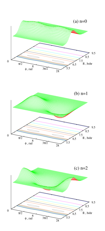
Figure 7: Wave functions multiplied by $R$ (in arbitrary units) for the lowest vibrational states of O₂-N₂, as functions of the intermolecular distance $R$ (bohr) and the torsional angle (radian). Contour plots of the PES are also shown in the bottom planes of the plots, with contour lines ranging from -14.5 to -0.5 meV, in steps of 2 meV. In all cases, the bending angles $\theta_{a}$ and $\theta_{b}$ have both been fixed at $\pi/2$. (a) $n=0$, real part, (b) $n=1$, imaginary part (c) $n=2$, real part; (the associated imaginary/real parts are zero).

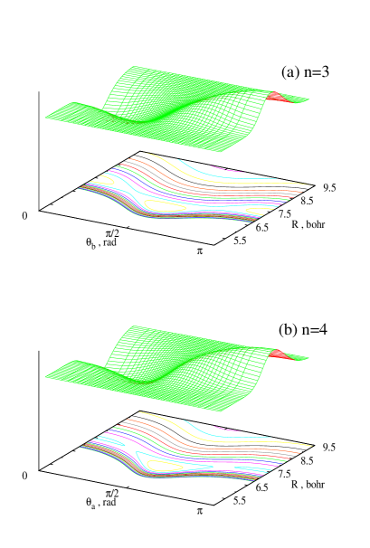
Figure 8: (a) Real part of the wave function multiplied by $R$ (in arbitrary units) of the third excited rotationless state ($n=$3) of O₂-N₂, as a function of $R$ (bohr) and $\theta_{b}$ (radian), with the bending angle $\theta_{a}$ fixed at $\pi/2$ and $\phi=$ 0. Imaginary part is zero. (b) As in (a), for $n=$4. In this case the wave function is shown versus $R$ and $\theta_{a}$, with $\theta_{b}=\pi/2$ and $\phi=$ 0. In this way, these states correspond to $T_{a}$ and $T_{b}$ configurations, respectively. Contour plots of the PES are also shown in the bottom planes of the plots, with contour lines ranging from -13.5 to -0.5 meV, in steps of 1 meV.

Table 6: Energies (in cm^-1) and symmetries of the lowest rotationally excited states of ¹⁶O₂-¹⁴N₂. Allowed states are given in boldface.

J=1		J=2		J=3
cm-1	Sym	cm-1	Sym	cm-1	Sym
-83.120	${\bf B_{1}^{\prime}}$	-82.804	${\bf B_{2}^{\prime}}$	-82.332	$B_{1}^{\prime\prime}$
-81.492	${\bf A_{2}^{\prime}}$	-81.185	${\bf A_{2}^{\prime}}$	-80.724	${\bf A_{2}^{{}^{\prime}}}$
-81.485	${\bf A_{1}^{\prime}}$	-81.165	${\bf A_{1}^{\prime}}$	-80.685	${\bf A_{1}^{{}^{\prime}}}$
-80.366	$A_{2}^{\prime\prime}$	-80.063	$A_{1}^{\prime\prime}$	-79.608	$A_{2}^{\prime\prime}$
-80.358	$A_{1}^{\prime\prime}$	-80.038	$A_{2}^{\prime\prime}$	-79.558	$A_{1}^{\prime\prime}$
-78.952	$B_{2}^{\prime\prime}$	-78.638	$B_{1}^{\prime\prime}$	-78.168	${\bf B_{2}^{\prime}}$
-78.211	$B_{1}^{\prime\prime}$	-78.516	$B_{2}^{\prime\prime}$	-78.057	${\bf B_{1}^{\prime}}$
-75.624	$A_{2}^{\prime\prime}$	-78.515	$B_{1}^{\prime\prime}$	-78.054	${\bf B_{2}^{\prime}}$
-74.240	$B_{1}^{\prime\prime}$	-77.900	$B_{2}^{\prime\prime}$	-77.433	${\bf B_{1}^{\prime}}$
-74.235	$B_{2}^{\prime\prime}$	-76.560	${\bf B_{2}^{\prime}}$	-76.095	$B_{1}^{\prime\prime}$
		-76.560	${\bf B_{1}^{\prime}}$	-76.095	$B_{2}^{\prime\prime}$
		-75.321	$A_{1}^{\prime\prime}$	-74.867	$A_{2}^{\prime\prime}$

In Table 5 we report the energies of the lowest bound states for total angular momentum $J=0$, together with their behavior under the operations of the symmetry group. Note that only the states shown in boldface are allowed. It can be noticed that there is a rather large density of states or, in other words, the vibrational motions involved have quite low frequencies. Analysis of the corresponding wave functions confirms the characteristic floppiness of this dimer. They have been obtained following the method of Thornley and Hutson Thornley and Hutson (1994), and setting the SF polar angles to ${\bf\hat{R}}$=$(\theta_{R},\phi_{R})$=(0,0), ${\bf\hat{r}}_{a}$=$(\theta_{a},\phi_{a})$=$(\theta_{a},\phi/2)$ and ${\bf\hat{r}}_{b}$=$(\theta_{b},\phi_{b})$=$(\theta_{b},-\phi/2)$. For the three lowest states ($n=0,1,2$), wave functions multiplied by $R$ ($R\Psi$) are shown in Fig. 7. They all have their largest amplitude for $\theta_{a}$=$\theta_{b}$=$\pi/2$ and, for these reasons, these wavefunctions are depicted as functions of the intermolecular distance, $R$, and the torsional angle, $\phi$, having fixed $\theta_{a}$ and $\theta_{b}$ at $\pi/2$. The ground state ($n$=0, Fig. 7(a)) is very delocalized with respect to the torsional motion, with a slight propensity for a X configuration. The first excited state ($n$=1, Fig.7(b)) exhibits a node for $\phi$=0 and has its maximum probability density at the X geometry. The second excited state also corresponds to an excitation of the torsional motion, in this case, the node is at $\phi$=$\pi/2$ and its geometry matches the H orientation.

The relatively large stability of the T-shape orientations in the O₂-N₂ PES (Fig. 3) is revealed in the structure of the higher excited states. Indeed, the third and fourth excited states have T-shape geometries. Wave functions for these states are presented in Fig. 8. The wave function of the $n$=3 state is depicted as a function of $R$ and $\theta_{b}$, where the $\theta_{a}$ and $\phi$ angles have been fixed to $\pi/2$ and 0, respectively (Fig. 8(a)). We have chosen to fix $\theta_{a}$ to $\pi/2$ because a maximum of the probability density is found precisely at this orientation. On the other hand, we have found that the amplitude is quite isotropic with respect to the torsional angle and have just chosen a representative planar configuration ($\phi=0$). It can be seen that this function displays a node at $\theta_{b}$=$\pi/2$ and a maximum amplitude for $\theta_{b}$=0, corresponding to a T_a configuration. Nevertheless, this angular mode displays a wide amplitude motion, since the amplitude is also significant for displacements out of the T_a geometry. The $n$=4 state has, on the other hand, a T_b geometry. The shape of its wave function as a function of $R$ and $\theta_{a}$ is given in Fig. 8(b), having fixed $\theta_{b}$ and $\phi$ to $\pi/2$ and 0, respectively. As the previos level, the $n$=4 state is also quite floppy with respect to motions of all the intermolecular degrees of freedom.

Finally, a list of some rotationally excited states ($J$= 1, 2, and 3) is reported in Table 6. It is worthwhile noting that the lowest levels of $J$= 1 and 2 are allowed states and their energies are lower than the lowest allowed states of $J=0$ (Table 5). This feature was already discussed by Aquilanti et al in their study of O₂-N₂ based in the Perugia-PESAquilanti et al. (2003).

Unfortunately, we cannot test present results against experiments as we were not able to find any publication on the spectroscopy of O₂-N₂. Aquilanti et al. Aquilanti et al. (2003) reported bound states calculated with their experimentally derived O₂-N₂ PESAquilanti et al. (1999). They reported $J=0$ states build up using odd and even values of $j$ for O₂ and N₂, respectively. The lowest energy levels are -98.1, -88.4 and -83.7 cm^-1, which should be compared with the corresponding present levels, -73.9, -67.2 and -67.1 cm^-1. As can be seen, differences between the ab initio PES and the Perugia-PES, discussed previously, become crucial for a quantitative prediction of the bound spectrum of this complex.

Present results can be also compared with the vibrational structure of the related dimers O₂-O₂ and N₂-N₂. First, O₂-N₂ bound states are quite different to those of O₂-O₂ in the singlet and triplet spin multiplicities, as, due to exchange interactions involving the two open-shell molecules, they exhibit a preference for the H geometry and are much more rigidCarmona-Novillo et al. (2012). However, the lowest vibrational states of O₂-N₂ are impressively similar to accurate calculations of O₂-O₂ in the quintet multiplicity Bartolomei et al. (2008a). In addition, the shape of the associated wave functions is very alike. Finally, comparing with calculations based on an experimentally derived PES for N₂-N₂Aquilanti et al. (2002), it is found that energies of the lowest bound states are rather similar: the three lowest energies are -79.9, -77.4 and -71.1. However, it was found that the ground state has a T-shaped geometry (in accordance with the features of the PES), whereas the first state in O₂-N₂ exhibiting such a geometry is the third vibrationally excited state.

V Concluding remarks

In the present paper state-of-the-art ab initio techniques have been applied to compute the ground state potential energy surface for the interaction of rigid N₂ and O₂ molecules in their ground electronic and vibrational states. The main results of this paper can be summarized as follows.

1. The potential energy surface for the O${}_{2}(^{3}\Sigma^{-}_{g})$ + N${}_{2}(^{1}\Sigma^{+}_{g})$ complex has a global minimum of 14.63 meV at $R=6.52$ bohr for the X ($D_{2d}$) geometry, and local minima of 14.05 meV at $R=7.44$ bohr and 12.58 meV at $R=7.52$ bohr for the T_a and T_b geometries, respectively.

2. Symmetry-adapted perturbation theory utilizing the DFT description of the isolated monomers was shown to work very well in comparison with the spin-restricted coupled cluster method with single, double, and noniterative triple excitations.

3. The accuracy of the computed potential was checked by comparison with the empirical potential from the Perugia group fitted to the measured integral cross sections. In general, relatively good agreement between the ab initio and empirical surfaces is found, the deviations ranging from 3% for the H geometry to 43% for the weakly bound L geometry. The present potential is more anisotropic than the experimentally derived potential.

4. The ab initio potential satisfactorily reproduces the measured integral cross sections. Both the glory oscillations as a function of the beam intensity and the absolute cross sections are in a (semi)quantitative agreement with the experimental data.

5. The ab initio potential also works well for the second virial coefficient of the O₂-N₂ mixture. Except for the two lowest temperatures, the present results are well within the experimental error bars leading to the best agreement to date for temperatures higher than the Boyle temperature. Second virial coefficients are also computed at temperatures where measured values are unavailable and, considering the accuracy of the present PES, they can be safely used to guide extrapolations at high temperature.

6. The analysis of the bound states of the complex reveals that the complex is floppy, and the nearly free rotors description is adequate. Unfortunately, no experimental data are available for comparison.

The potential energy surface reported in this work can be employed in future investigations such as studies of collision induced absorption or rotationally energy transfer in collisions.

References

- Lewis (1924) G. N. Lewis, J. Am. Chem. Soc. 46, 2027 (1924).
- Crawford et al. (1949) M. F. Crawford, H. L. Welsh, and J. L. Locke, Phys. Rev. 75, 1607 (1949).
- Frommhold (1994) L. Frommhold, Collision-induced Absorption in Gases (Cambridge Monographs on Atomic, Molecular and Chemical Physics, Cambridge University Press, 1994), ISBN 9780521393454.
- Abel and Frommhold (2013) M. Abel and L. Frommhold, Can. J. Phys. 91, 857 (2013).
- Klemperer and Vaida (2006) W. Klemperer and V. Vaida, Proc. Nat. Ac. Sci. 103, 10584 (2006).
- Bartolomei et al. (2008a) M. Bartolomei, E. Carmona-Novillo, M. I. Hernández, J. Campos-Martínez, and R. Hernández-Lamoneda, J. Chem. Phys. 128, 214304 (2008a).
- Bartolomei et al. (2008b) M. Bartolomei, M. I. Hernández, J. Campos-Martínez, E. Carmona-Novillo, and R. Hernández-Lamoneda, Phys. Chem. Chem. Phys 10, 5374 (2008b).
- Bartolomei et al. (2010) M. Bartolomei, E. Carmona-Novillo, J. Campos-Martínez, M. I. Hernández, and R. Hernández-Lamoneda, J. Chem. Phys. 133, 12431 (2010).
- Bartolomei et al. (2011) M. Bartolomei, E. Carmona-Novillo, M. I. Hernández, J. Campos-Martínez, and R. Hernández-Lamoneda, J. Comp. Chem. 32, 279 (2011).
- Gomez et al. (2007) L. Gomez, B. Bussery-Honvault, T. Cauchy, M. Bartolomei, D. Cappelletti, and F. Pirani, Chem. Phys. Lett. 445, 99 (2007).
- Jeziorski et al. (1994) B. Jeziorski, R. Moszynski, and K. Szalewicz, Chem. Rev. 94, 1887 (1994).
- Bussery-Honvault and Hartmann (2014) B. Bussery-Honvault and J.-M. Hartmann, J. Chem. Phys. 140, 054309 (2014), 054309:1-054309:6.
- Aquilanti et al. (2003) V. Aquilanti, M. Bartolomei, E. Carmona-Novillo, and F. Pirani, J. Chem. Phys. 118, 2214 (2003).
- Zuchowski et al. (2008) P. S. Zuchowski, R. Podeszwa, R. Moszynski, B. Jeziorski, and K. Szalewicz, J. Chem. Phys. 129, 084101 (2008), ISSN 0021-9606.
- van der Avoird and Brocks (1987) A. van der Avoird and G. Brocks, J. Chem. Phys. 87, 5346 (1987).
- Kendall et al. (1992) R. A. Kendall, T. H. Dunning, and R. J. Harrison, J. Chem. Phys. 96, 6796 (1992).
- Tao and Pan (1992) F. M. Tao and Y. K. Pan, J. Chem. Phys. 97, 4989 (1992).
- Adamo and Barone (1999) C. Adamo and V. Barone, J. Chem. Phys. 110, 6158 (1999).
- Dal (2005) Dalton, a molecular electronic structure program, release 2.0 (2005), see http://www.kjemi.uio.no/software/dalton/dalton.html.
- Fermi and Amaldi (1934) E. Fermi and G. Amaldi, Memorie della Classe di Scienze Fisiche, Matematiche e Naturali. R. Accademia D’Italia 6, 117 (1934).
- Tozer and Handy (1998) D. J. Tozer and N. C. Handy, J. Chem. Phys. 109, 10180 (1998).
- Żuchowski (2008) P. S. Żuchowski, Chem. Phys. Lett. 450, 203 (2008).
- (23) NIST Chemistry WebBook, NIST Standard Reference Database Number 69, ed. P. J. Linstrom and W. G. Mallard, 2007, http://WebBook.nist.gov.
- Bukowski et al. (2008) R. Bukowski, W. Cencek, P. Jankowski, M. Jeziorska, B. Jeziorski, S. A. Kucharski, V. F. Lotrich, A. J. Misquitta, R. Moszynski, K. Patkowski, et al., Sapt2008, version 2008.2, an ab initio program for many-body-symmetry-adapted perturbation theory of intermolecular interaction energies (2008), see http://www.physics.udel.edu/ szalewic/SAPT/index.html.
- Boys and Bernardi (1970) S. Boys and F. Bernardi, Mol. Phys. 19, 553 (1970).
- van Lenthe et al. (1987) J. H. van Lenthe, J. G. C. M. van Duijneveldt-van de Rijdt, and F. van Duijneveldt, Adv. Chem. Phys. 69, 521 (1987).
- Werner et al. (2006) H.-J. Werner, P. J. Knowles, R. Lindh, F. R. Manby, M. Schütz, P. Celani, T. Korona, G. Rauhut, R. D. Amos, A. Bernhardsson, et al., Molpro, version2006.1, a package of ab initio programs (2006), seehttp://www.molpro.net.
- Wormer and van der Avoird (1984) P. E. S. Wormer and A. van der Avoird, J. Chem. Phys. 81, 1929 (1984).
- Abramovitz and Stegun (1972) M. Abramovitz and I. A. Stegun, Handbook of Mathematical Functions (Dover, New York, 1972).
- Cwiok et al. (1992) T. Cwiok, B. Jeziorski, W. Kolos, R. Moszynski, J. Rychlewski, and K. Szalewicz, Chem. Phys. Lett. 195, 67 (1992).
- van der Avoird et al. (1980) A. van der Avoird, P. E. S. Wormer, F. Mulder, and R. M. Berns, in Topics in Current Chemistry (Springer, Berlin, Vol.93, Chapter 1, 1980), pp. 1–51.
- Heijmen et al. (1996) T. G. A. Heijmen, R. Moszynski, P. E. S. Wormer, and A. van der Avoird, Mol. Phys. 89, 81 (1996).
- Brunetti et al. (1981) B. Brunetti, G. Liuti, E. Luzzatti, F. Pirani, and F. Vecchiocattivi, J. Chem. Phys. 74, 6734 (1981).
- Cappelletti et al. (2008) D. Cappelletti, F. Pirani, B. Bussery-Honvault, L. Gómez, and M. Bartolomei, Phys. Chem. Chem. Phys 10, 4281 (2008).
- Bartolomei et al. (2008c) M. Bartolomei, D. Cappelletti, G. de Petris, M. M. Texidor, F. Pirani, M. Rosi, and F. Vecchiocattivi, Phys. Chem. Chem. Phys 10, 5993 (2008c).
- Thibault et al. (2009) F. Thibault, D. Cappelletti, F. Pirani, and M. Bartolomei, J. Phys. Chem. A 113, 14867 (2009).
- Cappelletti et al. (2002) D. Cappelletti, M. Bartolomei, F. Pirani, and V. Aquilanti, J. Phys. Chem. A 106, 10764 (2002).
- Schiff (1956) L. I. Schiff, Phys. Rev. 103, 443 (1956).
- Pirani and Vecchiocattivi (1982) F. Pirani and F. Vecchiocattivi, Mol. Phys. 45, 1003 (1982).
- Aquilanti et al. (1998) V. Aquilanti, D. Ascenzi, D. Cappelletti, M. de Castro-Vítores, and F. Pirani, J. Chem. Phys. 109, 3898 (1998).
- Pérez-Ríos et al. (2009) J. Pérez-Ríos, M. Bartolomei, J. Campos-Martínez, M. I. Hernández, and R. Hernández-Lamoneda, J. Phys. Chem. A 113, 14952 (2009).
- Bernstein and O’Brien (1965) R. B. Bernstein and T. J. P. O’Brien, Discuss. Faraday Soc. 40, 35 (1965).
- Bernstein and O’Brien (1967) R. B. Bernstein and T. J. P. O’Brien, J. Chem. Phys. 46, 1208 (1967).
- Pérez-Ríos et al. (2012) J. Pérez-Ríos, M. Bartolomei, J. Campos-Martínez, and M. I. Hernández, Chem. Phys. Lett. 522, 28 (2012), 28-32.
- Martin et al. (1982) M. Martin, R. Trengove, K. Harris, and P. Dunlop, Aust. J. Chem. 35, 1525 (1982).
- Fostiropoulos et al. (1988) K. Fostiropoulos, G. Natour, J. Sommer, and B. Schramm, Ber. Bunsenges. Phys. Chem. 92, 925 (1988).
- Pack (1983) R. T. Pack, J. Chem. Phys. 78, 7217 (1983).
- Eubank and Hall (1990) P. T. Eubank and K. R. Hall, AIChE Journal 36, 1661 (1990).
- Bunker (1979) P. R. Bunker, Molecular Symmetry and Spectroscopy (Academic Press Inc., 1979).
- Green (1975) S. Green, J. Chem. Phys. 62, 2271 (1975).
- van der Avoird et al. (1994) A. van der Avoird, P. Wormer, , and R. Moszynski, Chem. Rev. 94, 1931 (1994).
- Hutson (1994) J. M. Hutson, Comp. Phys. Comm. 84, 1 (1994).
- Alexander and DePristo (1977) M. H. Alexander and A. E. DePristo, J. Chem. Phys. 66, 2166 (1977).
- Brown and Carrington (2003) J. Brown and A. Carrington, Rotational Spectroscopy of Diatomic Molecules (Cambridge University Press, 2003).
- J. M. Hutson (1993) BOUND. J. M. Hutson (1993), computer Code, Version 5, distributed by Collaborative Computational Project no. 6 of the Science and Engineering Research Council (UK).
- Manolopoulos (1986) D. E. Manolopoulos, J. Chem. Phys. 85, 6425 (1986).
- Johnson (1973) B. R. Johnson, J. Comp. Phys. 13, 445 (1973).
- Thornley and Hutson (1994) A. E. Thornley and J. M. Hutson, J. Chem. Phys. 101, 5578 (1994).
- Aquilanti et al. (1999) V. Aquilanti, D. Ascenzi, M. Bartolomei, D. Cappelletti, S. Cavalli, M. de Castro Vitores, and F. Pirani, J. Am. Chem. Soc. 121, 10794 (1999).
- Carmona-Novillo et al. (2012) E. Carmona-Novillo, M. Bartolomei, M. I. Hernández, J. Campos-Martínez, and R. Hernández-Lamoneda, J. Chem. Phys. 137, 114304 (2012).
- Aquilanti et al. (2002) V. Aquilanti, M. Bartolomei, D. Cappelletti, E. Carmona-Novillo, and F. Pirani, J. Chem. Phys. 117, 615 (2002).