Turbulent mixing of a slightly supercritical Van der Waals fluid at Low-Mach number

Abstract

Supercritical fluids near the critical point are characterized by liquid-like densities and gas-like transport properties. These features are purposely exploited in different contexts ranging from natural products extraction/fractionation to aerospace propulsion. Large part of studies concerns this last context, focusing on the dynamics of supercritical fluids at high Mach number where compressibility and thermodynamics strictly interact. Despite the widespread use also at low Mach number, the turbulent mixing properties of slightly supercritical fluids have still not investigated in detail in this regime. This topic is addressed here by dealing with Direct Numerical Simulations (DNS) of a coaxial jet of a slightly supercritical Van der Waals fluid. Since acoustic effects are irrelevant in the Low Mach number conditions found in many industrial applications, the numerical model is based on a suitable low-Mach number expansion of the governing equation. According to experimental observations, the weakly supercritical regime is characterized by the formation of finger-like structures– the so-called ligaments –in the shear layers separating the two streams. The mechanism of ligament formation at vanishing Mach number is extracted from the simulations and a detailed statistical characterization is provided. Ligaments always form whenever a high density contrast occurs, independently of real or perfect gas behaviors. The difference between real and perfect gas conditions is found in the ligament small-scale structure. More intense density gradients and thinner interfaces characterize the near critical fluid in comparison with the smoother behavior of the perfect gas. A phenomenological interpretation is here provided on the basis of the real gas thermodynamics properties.

I Introduction

A supercritical fluid is a phase of matter with no sharp transition between high, liquid-like density states and low, gas-like density states that exists at pressures and temperatures higher than those of the critical point. It consists of a unique hybrid state intermediate between liquid and gas where no surface tension acts at density interfaces. In certain regions of the phase diagram, supercritical fluids exhibit liquid-like density and gas-like transport properties that diverge approaching the critical point. These peculiar features make supercritical fluids attractive in several industrial and technological applications from space propulsions to chemical extraction processes palmer1995applications ; perrut2000supercritical ; fages2004particle ; brunner2010applications .

The frequent use of supercritical fluids in aerospace propulsion devices, as in liquid rocket engines, motivated a substantial part of the studies in the literature. Indeed, numerous experimental investigations on supercritical fluids chetalcoy ; segpol ; royjolseg ; MayTelBraSChHus ; mayschschsch have been addressing turbulent mixing properties, like Nitrogen/Heptane systems in experiments devoted to the basic understanding of mixing or Hydrogen/Oxygen systems for applications to combustion. Interesting reviews on these issues are Refs bellan2000supercritical, and zonyan, which provide the state-of-the-art up to 2000. In recent years numerical simulations also addressed supercritical mixing by investigating temporal mixing layers MilHarBel ; okobel ; okobel1 and turbulent jet flows oef . Aiming at aerospace propulsion applications, all these studies considered supercritical flows with moderately high Mach numbers where acoustic effects and pressure fluctuations are crucial MilHarBel .

On the other hand many technological applications often employ fluids at low speed. In industrial applications, supercritical fluids are frequently used in place of CFC for cooling linghejon , to sterilize biological materials checinska2011sterilization , for textiles cleaning, and for electronics components degreasing weibel2003overview . Supercritical fluids are also widely adopted for chemical extraction, e.g. to extract substances from foods king1996supercritical ; mendiola2013supercritical in processes like decaffeination by $CO_{2}$ capuzzo2013supercritical . For these cases at vanishing Mach number, where acoustic effects are negligible, much less attention has been paid to turbulent mixing between a faster and a slower stream of even a single-component supercritical fluid. It turns out that, when dealing with supercritical flows, the computational difficulties known to arise in strongly subsonic flows, notably the increasingly stiff behavior of the compressible Navier-Stokes equations at increasing sound speed majset ; vol , still need to be addressed in detail. A major aim of the present work is to develop a consistent treatment of a supercritical fluid at small Mach number capable of being implemented in efficient numerical simulations of turbulent mixing.

In this context, the Low-Mach expansion, developed by Majda & Sethian majset for perfect-gas reacting flows, is certainly a fundamental starting point. However their formulation needs to be substantially rearranged to allow the extension to real gas conditions. The original part of the relevant asymptotic expansion is presented here by focusing on the special case of Van der Waals fluids. It is then a straightforward exercise adapting it to other cases of practical interest, like to the widespread Peng-Robinson equation of state penrob .

Beside introducing the low Mach number expansion, the primary intent of the paper is investigating the peculiar features of the turbulent mixing of a single-component Van der Waals fluid at vanishing Mach number and slightly supercritical pressure. The issue is addressed by focusing on a co-axial jet with two streams at different temperatures and velocities. Data from Direct Numerical Simulations (DNS) of real and perfect gas are compared to highlight the effect induced by the real gas thermodynamics. Similarly to the high Mach number case royjolseg ; MayTelBraSChHus , the weakly supercritical regime is characterized by the formation of finger-like structures (ligaments) in the shear layers separating the two streams. We show that ligaments always form whenever a high density contrast occurs, independently of real or perfect gas conditions. The ligament small scale structure is found to distinguish the real from the perfect gas behavior with more intense density gradients and thinner interfaces characterizing the near-critical fluid in comparison with the smoother behavior of the perfect gas.

The paper is organized as follows. Section § II is dedicated to the generalized Low Mach number expansion for real-gas flows. Section § III deals with the specific aspects of the Van der Waals model. In section § IV the variable-density turbulent coaxial jet simulations are presented, discussing the relevant aspects of the solution algorithm. The detailed physics of the near-critical jet dynamics is illustrated in § V that provides the main physical results of the paper. Final comments and conclusions are eventually reported in § VI. A few Appendices are included at the end, to allow the illustration of certain technical aspects without interrupting the main stream of the discussion.

II The Low-Mach number formulation for a generic equation of state

In the original derivation of the low-Mach number approximation of the fully compressible, reacting Navier-Stokes equations, Majda & Sethian majset employed the perfect gas equation of state to describe the thermodynamic behavior of the fluid. The original procedure described in that seminal paper heavily relies on the particularly simple and specific form of the equation of state. However, when dealing with near-critical conditions, the equation of state should be generalized to treat more general cases and allow the use of the Van der Waals model or other appropriate real gas descriptions.

Since deriving the approximation under these more general conditions requires a different manipulation of the equations, the basic procedure is here briefly outlined.

The fully compressible, single component Navier-Stokes equations read as

$$\displaystyle{\frac{\partial\rho^{*}}{\partial t^{*}}}+{\bf\nabla}^{\,*}\cdot(\rho^{*}{\bf u}^{*})=0\,,$$ (1)

$$\displaystyle{\frac{\partial(\rho^{*}{\bf u}^{*})}{\partial t^{*}}}+{\bf\nabla}^{\,*}\cdot(\rho^{*}{\bf u}^{*}\otimes{\bf u}^{*})={\bf\nabla}^{\,*}\cdot{\bf\Sigma}^{*}-{\bf\nabla}^{\,*}p^{*}+{\bf f}^{*}\,,$$ (2)

$$\rho^{*}\left(\frac{\partial{\cal U}^{*}}{\partial t^{*}}+{\bf u}^{*}\cdot{\bf\nabla}^{\,*}{{\cal U}^{*}}\right)=-p^{*}{\bf\nabla}^{\,*}\cdot{\bf u}^{*}+{\bf\Sigma}^{*}:{\bf\nabla}^{\,*}\otimes{\bf u}^{*}-{\bf\nabla}^{\,*}\cdot{\bf q}^{*}\,,$$ (3)

$$\displaystyle{\frac{\partial(\rho^{*}Y^{*})}{\partial t^{*}}}+{\bf\nabla\cdot}(\rho^{*}{\bf u}^{*}Y^{*})={\bf\nabla}^{\,*}\cdot({\cal D}^{*}{\bf\nabla}^{\,*}Y^{*})\,,$$ (4)

$$p^{*}=p^{*}(\theta^{*},\rho^{*})\,,$$ (5)

$${\cal U}^{*}={\cal U}^{*}(\theta^{*},\rho^{*})\,,$$ (6)

where the asterisk denotes dimensional variables. In the equations, $t^{*}$, $\rho^{*}$, $p^{*}$, $\theta^{*}$, ${\bf u}^{*}$ are time, density, pressure, temperature and velocity, respectively with ${\bf\nabla}^{*}$ the spatial gradient and $\otimes$ the tensor product. ${\bf\Sigma}^{*}=\mu^{*}[({\bf\nabla}^{\,*}\otimes{\bf u}^{*}+({\bf\nabla}^{\,*}\otimes{\bf u}^{*})^{T})-\left({\mu_{B}^{*}}/{\mu^{*}}-{2}/{3}\right)({\bf\nabla}^{\,*}\cdot{\bf u}^{*})\,{\bf I}]$ is the viscous stress tensor, $\mu^{*}(\theta^{*})$ and $\mu^{*}_{B}(\theta^{*})$ are the temperature dependent dynamic and bulk viscosity, respectively, and ${\bf f}^{*}=-\rho^{*}g^{*}{\bf e}_{z}$ is the gravitational force (with ${\bf e}_{z}$ the vertical unit vector). For simplicity, in eq. (3) the heat flux ${\bf q}^{*}$ is assumed to follow the Fourier law, ${\bf q}^{*}=-k^{*}(\theta^{*})\,{\bf\nabla}^{\,*}\theta^{*}$ as appropriate for single component fluids. ${\cal U}^{*}$ is the internal energy per unit mass, obeying an equation of state in terms of temperature and density, eq. (6). Equation (4) is the convection-diffusion equation for a generic passive scalar, like a tracer that is mixed by the flow. Finally, eq. (5) is a generic equation of state expressing the pressure in terms of density $\rho^{*}$ and temperature $\theta^{*}$. The system can be easily extended to deal with multi-component reactive mixtures by including additional convection-diffusion-reaction equations for each species and by considering a more complete transport model for heat and mass fluxes, see e.g. Ref law, . The extension of the Low Mach number expansion to be introduced below to the more general multi-component, reactive case is straightforward and will not be discussed further in the following.

The Low Mach number expansion is better performed starting from the dimensionless system. After selecting a characteristic length $\ell^{*}_{R}$, a speed $|{\bf u}^{*}_{R}|$, a pressure $p^{*}_{R}$ and a density $\rho^{*}_{R}$, the other reference quantities follows as

$$t^{*}_{R}=\frac{l^{*}_{R}}{|{\bf u}^{*}_{R}|},\quad{\cal U}^{*}_{R}=\frac{p^{*}_{R}}{\rho^{*}_{R}},\quad\theta^{*}_{R}=\theta^{*}_{R}\left(p^{*}_{R},\rho^{*}_{R}\right)$$ (7)

where the characteristic temperature $\theta^{*}_{R}$ is expressed as a function of reference pressure and density through the pressure equation of state (5), see also § III. The dimensionless system reads

$$\displaystyle{\frac{\partial\rho}{\partial t}}+{\bf\nabla\cdot}(\rho{\bf u})=0$$ (8)

$$\displaystyle{\frac{\partial(\rho{\bf u})}{\partial t}}+{\bf\nabla\cdot}(\rho{\bf u}\otimes{\bf u})=\frac{1}{\mbox{{Re}}}{\bf\nabla\cdot}{\bf\Sigma}-\frac{1}{\gamma_{R}\widehat{Ma}^{2}}{\bf\nabla}p-\frac{1}{Fr^{2}}\rho{\bf e}_{z}$$ (9)

$$\rho\left(\frac{\partial{\cal U}}{\partial t}+{\bf u}\cdot{\bf\nabla}{{\cal U}}\right)=-p{\bf\nabla\cdot}{\bf u}+\frac{\gamma_{R}\widehat{Ma}^{2}}{\mbox{{Re}}}{\bf\Sigma}:{\bf\nabla}\otimes{\bf u}+{\frac{c_{pR}^{*}}{{\cal ZR}_{m}^{*}}}\frac{1}{\mbox{{Re}}\,\mbox{{Pr}}}{\bf\nabla\cdot}\left(k{\bf\nabla}\theta\right)$$ (10)

$$\displaystyle{\frac{\partial(\rho Y)}{\partial t}}+{\bf\nabla\cdot}(\rho{\bf u}Y)=\frac{1}{\mbox{{Re}}Sc}{\bf\nabla\cdot}({\cal D}{\bf\nabla}Y)$$ (11)

$$p=p(\theta,\rho)$$ (12)

$${\cal U}={\cal U}(\theta,\rho)\,,$$ (13)

where the relevant dimensionless parameters are

$$\widehat{Ma}=\frac{\left|{\bf u}^{*}_{R}\right|}{\sqrt{{\gamma_{R}p^{*}_{R}}/{\rho^{*}_{R}}}},\quad\mbox{{Re}}=\frac{\left|{\bf u}^{*}_{R}\right|\,\ell^{*}_{R}\,\rho^{*}_{R}}{\mu^{*}_{R}},\quad\mbox{{Pr}} =\frac{{c_{p}}^{*}_{R}\mu^{*}_{R}}{k^{*}_{R}},$$

$$Fr=\frac{\left|{\bf u}^{*}_{R}\right|}{\sqrt{\ell^{*}_{R}g^{*}}},\quad Sc=\frac{\mu_{R}}{{\cal D}_{R}\rho^{*}_{R}},$$

with ${c^{*}_{p}}_{R}=c^{*}_{p}(\theta_{R}^{*},\rho_{R}^{*})$ being $c^{*}_{p}=\partial\left[{\cal U}^{*}+p^{*}/\rho^{*}\right]/\partial\theta^{*}_{|p^{*}}$ the constant-pressure specific heat coefficient, ${\cal R}_{m}^{*}$ is the gas constant, $Z=p_{R}^{*}/({\cal R}_{m}^{*}\theta_{R}^{*}\rho_{R}^{*})$ is the compressibility factor, and $k^{*}_{R}$ and $\mu^{*}_{R}$ the thermal diffusion coefficient and the dynamic viscosity, respectively, evaluated at the reference temperature $\theta^{*}_{R}$. $\widehat{Ma}$ takes the role of the Mach number, even if the quantity in the denominator does not directly coincide with the sound speed at reference thermodynamic conditions, since in general, for a real gas, $c_{R}^{2}=\partial p^{*}/\partial\rho^{*}_{|S^{*}}(\theta_{R}^{*},\rho_{R}^{*})\neq\gamma_{R}p_{R}^{*}/\rho_{R}^{*}$ with $\gamma_{R}$ the ratio of constant pressure to constant volume specific heat and $c_{R}$ the actual sound speed in the reference conditions.

The Low Mach number formulation, Ref majset, , amounts to introducing the asymptotic expansion

$${\bf f}({\bf x},t)={\bf f}_{0}({\bf x},t)+{\bf f}_{2}({\bf x},t)\widehat{Ma}^{2}+O(\widehat{Ma}^{4})\,.$$ (15)

for the generic variable into system (8)-(13). After grouping together terms with the same power in the Mach number and requiring that the resulting equations should be identically satisfied for any, sufficiently small Mach number, the system of equations governing the different terms in expansion (15) is readily obtained.

The zero-th order contribution to the mass conservation equation is

$${\frac{\partial\rho_{0}}{\partial t}}+{\bf\nabla\cdot}({\rho}_{0}{{\bf u}}_{0})=0\ .$$ (16)

The same procedure applied to the momentum conservation provides a first contribution formally diverging like $1/\widehat{Ma}^{2}$. Removing this low Mach number divergence yields the equation

$${\bf\nabla}p_{0} =0\,\Rightarrow\,p_{0}=p_{0}(t)\,,$$ (17)

that implies a spatially constant zero-th order (thermodynamic) pressure. A second contribution arises at zero-th order in the Mach number and is given by

$$\displaystyle{\frac{\partial({\rho}_{0}{{\bf u}}_{0})}{\partial t}}+{\bf\nabla\cdot}({\rho}_{0}{{\bf u}}_{0}\otimes{{\bf u}}_{0}) =\frac{1}{\mbox{{Re}}}{\bf\nabla\cdot}{\bf\Sigma}_{0}-{\bf\nabla}p_{2}+\frac{\rho_{0}}{Fr^{2}}{\bf e}_{z}\,,$$ (18)

where $p_{2}$ is the second order (hydrodynamic) pressure majset . Analogously, the zero-th order equation for the transported scalar follows as

$$\displaystyle{\frac{\partial(\rho_{0}Y_{0})}{\partial t}}+{\bf\nabla\cdot}(\rho_{0}{{\bf u}}_{0}Y_{0}) =\frac{1}{\mbox{{Re}}Sc}{\bf\nabla\cdot}({\cal D}{\bf\nabla}Y_{0})\ .$$ (19)

In order to complete the asymptotic expansion for real gases it is worth recasting the energy equation (10) in terms of temperature exploiting the equation of state (13) (more details are given in Appendix C),

$$\rho\frac{c_{v}^{*}}{{\cal R}_{m}^{*}}\frac{D\theta}{Dt}=-Z\theta\left.\frac{\partial p}{\partial\theta}\right|_{\rho}\,{\bf\nabla\cdot}{\bf u}+Z\frac{\gamma_{R}\widehat{Ma}^{2}}{\mbox{{Re}}}\,{\bf\Sigma}:{\bf\nabla}{\bf u}+\frac{c_{p}^{*}}{{\cal R}_{m}^{*}}\frac{1}{\mbox{{Re}}\,\mbox{{Pr}}}{\bf\nabla\cdot}\left(k{\bf\nabla}\theta\right)\,,$$ (20)

where $c_{v}^{*}=\left.\partial{{\cal U}^{*}}/\partial{\theta^{*}}\right|_{v^{*}}$ is the constant-volume specific heat coefficient. Exploiting the Low-Mach number expansion of the temperature equation, the zero-order contribution follows as

$$\rho_{0}\frac{c_{v0}^{*}}{{\cal R}_{m}^{*}}\frac{D\theta_{0}}{Dt}=-Z\theta_{0}\left.\frac{\partial p_{0}}{\partial\theta_{0}}\right|_{\rho_{0}}\,{\bf\nabla\cdot}{\bf u_{0}}+\frac{c_{p0}^{*}}{{\cal R}_{m}^{*}}\frac{1}{\mbox{{Re}}\,\mbox{{Pr}}}{\bf\nabla\cdot}\left(k_{0}{\bf\nabla}\theta_{0}\right)$$ (21)

where $c_{v0}^{*}=c_{v}^{*}\left(\theta^{*}_{R}\theta_{0},\rho^{*}_{R}\rho_{0}\right)$ and $c_{p0}^{*}=c_{p}^{*}\left(\theta^{*}_{R}\theta_{0},\rho^{*}_{R}\rho_{0}\right)$. The equation is further manipulated by expressing the temperature derivative on the left-hand side though the mass-conservation equation, where the density is expressed as $\rho^{*}=\rho^{*}(\theta^{*},p^{*})$, eq. (5),

$$\frac{1}{\rho_{0}}\left(\frac{D\rho}{Dt}\right)_{0} =\left(\frac{\theta^{*}_{R}}{\rho^{*}}\frac{\partial\rho^{*}}{\partial\theta^{*}}_{|_{p^{*}}}\right)_{\begin{subarray}{c}p^{*}=p^{*}_{R}p_{0}\\ \theta^{*}=\theta^{*}_{R}\theta_{0}\end{subarray}}\left(\frac{D\theta}{Dt}\right)_{0}+\left(\frac{p^{*}_{R}}{\rho^{*}}\frac{\partial\rho^{*}}{\partial p^{*}}_{|_{\theta^{*}}}\right)_{\begin{subarray}{c}\theta^{*}=\theta^{*}_{R}\theta_{0}\\ p^{*}=p^{*}_{R}p_{0}\end{subarray}}\left(\frac{Dp}{Dt}\right)_{0}$$

$$=-\alpha_{0}\left(\frac{D\theta}{Dt}\right)_{0}+\beta_{0}\left(\frac{Dp}{Dt}\right)_{0}=-{\bf\nabla\cdot}{\bf u}_{0}\,,$$ (22)

where the dimensionless thermal expansion and isothermal compressibility coefficients, $\alpha_{0}(\theta_{0},p_{0})$ and $\beta_{0}(\theta_{0},p_{0})$, respectively, are implicitly defined by comparing the second and the third member of the equation. Substituting the material derivative of temperature from equation (22) into (21) yields

$$\rho_{0}\frac{c_{v0}^{*}}{{\cal R}_{m}^{*}}\frac{\beta_{0}}{\alpha_{0}}\frac{Dp_{0}}{Dt}+\frac{c_{v0}^{*}}{{\cal R}^{*}_{m}}\frac{\rho_{0}}{\alpha_{0}}{\bf\nabla\cdot}{\bf u}=-Z\theta_{0}\left.\frac{\partial p_{0}}{\partial\theta_{0}}\right|_{v_{0}}\,{\bf\nabla\cdot}{\bf u_{0}}+\frac{c_{p0}^{*}}{{\cal R}_{m}^{*}}\frac{1}{\mbox{{Re}}\,\mbox{{Pr}}}{\bf\nabla\cdot}\left(k_{0}{\bf\nabla}\theta_{0}\right)\,,$$ (23)

where the zero-th order contribution to the pressure term depends only on time, $Dp_{0}/Dt=dp_{0}/dt$, as shown in eq. (17). The velocity divergence then reads

$${\bf\nabla\cdot}{\bf u_{0}}=\frac{\displaystyle-\rho_{0}\frac{c_{v0}^{*}}{{\cal R}_{m}^{*}}\frac{\beta_{0}}{\alpha_{0}}\frac{dp_{0}}{dt}+\frac{c_{p0}^{*}}{{\cal R}_{m}^{*}}\frac{1}{\mbox{{Re}}\,\mbox{{Pr}}}{\bf\nabla\cdot}\left(k_{0}{\bf\nabla}\theta_{0}\right)}{\displaystyle\frac{c_{v0}^{*}}{{\cal R}_{m}^{*}}\frac{\rho_{0}}{\alpha_{0}}+Z\theta_{0}\left.\frac{\partial p_{0}}{\partial\theta_{0}}\right|_{\rho_{0}}}\ .$$ (24)

Summarizing, the complete system in the zero-th order approximation is

$${\displaystyle\frac{\partial\rho_{0}}{\partial t}}+{\bf\nabla\cdot}(\rho{\bf u})_{0}=0$$ (25)

$$\displaystyle{\frac{\partial(\rho{\bf u})_{0}}{\partial t}}+{\bf\nabla\cdot}[(\rho{\bf u})_{0}\otimes{\bf u}_{0}]=\frac{1}{\mbox{{Re}}}{\bf\nabla\cdot}{\bf\Sigma}_{0}-{\bf\nabla}p_{2}+\frac{1}{Fr^{2}}\rho_{0}{\bf e}_{z}$$ (26)

$${\bf\nabla\cdot}{\bf u_{0}}=\frac{\displaystyle-\rho_{0}\frac{c_{v0}^{*}}{{\cal R}_{m}^{*}}\frac{\beta_{0}}{\alpha_{0}}\frac{dp_{0}}{dt}+\frac{c_{p0}^{*}}{{\cal R}_{m}^{*}}\frac{1}{\mbox{{Re}}\,\mbox{{Pr}}}{\bf\nabla\cdot}\left(k_{0}{\bf\nabla}\theta_{0}\right)}{\displaystyle\frac{c_{v0}^{*}}{{\cal R}_{m}^{*}}\frac{\rho_{0}}{\alpha_{0}}+Z\theta_{0}\left.\frac{\partial p_{0}}{\partial\theta_{0}}\right|_{\rho_{0}}}$$ (27)

$$\displaystyle{\frac{\partial(\rho_{0}Y_{0})}{\partial t}}+{\bf\nabla\cdot}(\rho_{0}{{\bf u}}_{0}Y_{0})=\frac{1}{\mbox{{Re}}Sc}{\bf\nabla\cdot}({\cal D}{\bf\nabla}Y_{0})$$ (28)

$$p_{0}(t)=p\left[\theta_{0}({\bf x},t),\rho_{0}({\bf x},t)\right]\,.$$ (29)

The crucial features of the system of equations we arrived at are worth begin emphasized: i) Zero-th order density $\rho_{0}({\bf x},t)$ and temperature $\theta_{0}({\bf x},t)$ are not independent fields since they are locally coupled through the equation of state (29). Indeed the time evolution of the thermodynamic pressure $p_{0}(t)$ follows by integrating (27) over the, generally time dependent, flow domain ${\cal D}(t)$ and accounting for the boundary conditions on the normal velocity component and on the temperature,

$$\frac{dp_{0}}{dt}\int_{{\cal D}(t)}\rho_{0}\frac{c_{v0}^{*}}{{\cal R}_{m}^{*}}\frac{\beta_{0}}{\alpha_{0}}dV= \int_{\partial{\cal D}(t)}\frac{c_{p0}^{*}}{{\cal R}_{m}^{*}}\frac{1}{\mbox{{Re}}\,\mbox{{Pr}}}k_{0}\frac{\partial\theta_{0}}{\partial n}dS-\int_{{\cal D}(t)}\frac{1}{\mbox{{Re}}\,\mbox{{Pr}}}k_{0}{\bf\nabla}\theta_{0}\cdot\nabla\left(\frac{c_{p0}^{*}}{{\cal R}_{m}^{*}}\right)dV$$ (30)

$$-\int_{{\cal D}(t)}\left(\frac{c_{v0}^{*}}{{\cal R}_{m}^{*}}\frac{\rho_{0}}{\alpha_{0}}+Z\theta_{0}\left.\frac{\partial p_{0}}{\partial\theta_{0}}\right|_{\rho_{0}}\right)dV\int_{\partial{\cal D}(t)}{\bf u_{0}}\cdot{{\bf n}}dS\ .$$

Stepwise integration allows to determine $p_{0}(t)$ and to eliminate either density or temperature in favour of the other field through (29). In particular, the pressure is constant for the present problem in an unbound domain, i.e. $p_{0}(t)=p_{0}=const$. ii) Acoustic waves are implicitly filtered out of the system, since the equation of state for pressure only enters at the lowest order, where pressure is spatially constant. The thermodynamic pressure is decoupled in this way from turbulence- and thermal-induced spatial variations of density, preventing acoustic waves from propagating in the medium. These effects can possibly be consistently recovered at next orders in the approximation. iii) The fluid density is allowed to change both in space and time to comply with thermal expansion effects– heat release due to combustion and heat transfer are perfectly consistent within the assumed approximation limits. iv) No assumption is made as concerning the thermodynamic model of the fluid. This is essential in view of our present aim of modelling turbulent mixing of slightly supercritical fluids. For the sake of definiteness, it should be stressed that resonance effects associated with thermo-acoustic coupling cannot be consistently dealt with within the range of validity of the present approximation, since, by non-linear coupling, they bring acoustics in foreground calling for a complete modelling of wave propagation.

III Thermodynamic assumptions

As anticipated in the § I, the perfect gas equation of state is not suitable to describe the thermodynamic behavior close to the critical point. Indeed the Van der Waals equation of state is presumably the simplest extension of the perfect gas model able to consistently deal with the thermodynamics of a diatomic gas at a slightly super-critical pressure. It will be hereafter assumed for its simplicity in the present application of the Low-Mach number expansion which, however, can be easily adapted to more general cases, like e.g. the Peng-Robinson equation of state penrob , see Appendix A.2.

The Van der Walls theory is directly derived from statistical mechanics, see e.g. Ref zhu, , and allows a complete and straightforward thermodynamic characterization of the gas starting from the Helmholtz free energy $f^{*}=-Nk_{b}\theta\ln\left(\cal Z^{*}\right)$ of the system expressed in terms of the canonical partition function ${\cal Z}^{*}(N,V,\theta)$ of the corresponding atomistic model. Here $N$ is the number of gas molecules, $V$ the volume and $k_{B}$ the Boltzmann constant, see Appendix A for a brief review of the subject. The pressure equation of state follows as

$$p^{*}=-\left.\frac{\partial f^{*}}{\partial V^{*}}\right|_{\theta^{*},N}=\frac{{\cal R}_{m}^{*}\theta^{*}\rho^{*}}{1-b^{\prime*}\rho^{*}}-a^{\prime*}\rho^{*2}\,,$$ (31)

where $a^{\prime*}$ and $b^{\prime*}$ are the Van der Waals coefficients that account for intermolecular forces and excluded volume, respectively. Thermal expansion and isothermal compressibility coefficients, $\alpha^{*}$ and $\beta^{*}$ respectively,

$$\alpha^{*}=-\frac{{\cal R}_{m}^{*}}{2a^{\prime*}\rho^{*}-3a^{\prime*}b^{\prime*}\rho^{*2}-p^{*}b^{\prime*}-{\cal R}_{m}^{*}\theta^{*}}$$

$$\beta^{*}=\frac{\left(1-b^{\prime*}\rho^{*}\right)/\rho^{*}}{2a^{\prime*}\rho^{*}-3a^{\prime*}b^{\prime*}\rho^{*2}-p^{*}b^{\prime*}-{\cal R}_{m}^{*}\theta^{*}}$$

follow directly from the pressure equation of state. All these thermodynamic relationships can be expressed in dimensionless form. Assuming $p=p_{0}+{\cal O}\left(\widehat{Ma}^{2}\right)$, with similar expressions for $\theta$ and $\rho$, leads to the leading order contributions in the Low Mach number expansion for pressure, thermal expansion and isothermal compressibility,

$$p_{0} =\frac{\theta_{0}\rho_{0}}{Z(1-b^{\prime}\rho_{0})}-a^{\prime}\rho_{0}^{2}\,,$$ (32)

$$\alpha_{0} =-\frac{1}{Z\left(2a^{\prime}\rho_{0}-3a^{\prime}b^{\prime}\rho_{0}^{2}-p_{0}b^{\prime}\right)-\theta_{0}}$$ (33)

$$\beta_{0} =\frac{\left(1-b^{\prime}\rho_{0}\right)/\rho_{0}}{2a^{\prime}\rho_{0}-3a^{\prime}b^{\prime}\rho_{0}^{2}-p_{0}b^{\prime}-\theta_{0}/Z}$$ (34)

where $a^{\prime}=a^{\prime*}\rho_{R}^{*2}/p_{R}^{*}$ and $b^{\prime}=b^{\prime*}\rho_{R}^{*}$.

Applying the analysis presented in section § II to the Van der Waals equation of state, most of the equations in system (25)-(29) remain unchanged, while velocity divergence and pressure equation of state become

$${\bf\nabla\cdot}{{\bf u}}_{0} ={\displaystyle\frac{1}{Z\,p_{0}}}\left[\frac{c_{p0}^{*}}{{\cal R}_{m}^{*}}\frac{1}{\mbox{{Re}}\mbox{{Pr}}}{\bf\nabla\cdot}(k{\bf\nabla}\theta)_{0}\right]\left[\frac{1}{\displaystyle{1+\frac{\left(\gamma-2\right)a\rho_{0}^{2}}{p_{0}\gamma}+\frac{2a^{\prime}b^{\prime}\rho_{0}^{3}}{p_{0}\gamma}}}\right]$$ (35)

$$\theta_{0} =Z\,{\displaystyle\frac{p_{0}}{\rho_{0}}\left(1+a^{\prime}\frac{\rho_{0}^{2}}{p_{0}}\right)\left(1-b^{\prime}\rho_{0}\right)}\,.$$ (36)

In eq. (35) $\gamma=c_{p0}^{*}/c_{v0}^{*}$ and the spatially constant pressure has been assumed constant also in time, $p_{0}(t)={\rm const}$, as appropriate for a free jet configuration where the discharge pressure is a known parameter. Overall, the system is formed by seven equations in the seven unknowns $\rho_{0}$, ${{\bf u}}_{0}$, $p_{2}$, $Y_{0}$ and $\theta_{0}$. Peculiar feature is the presence of the hydrodynamic pressure $p_{2}$ in the momentum equation majset . Under this respect, the system is similar to the incompressible Navier-Stokes equations where the pressure takes the mathematical role of a Lagrange multiplier that allows to enforce the constraint (35) on the velocity.

As a final comment on the mathematical model, we like stress once more that the same machinery would work in the same way also for different gas models.

IV Numerics and physical parameters

The DNS of a coaxial jet of a Van der Waals gas –hereafter referred to as real-gas– is performed employing cylindrical coordinates $\left(r,\varphi,z\right)$, with $z$ the axial coordinate, $r$ the radial coordinate in the transverse plane and $\varphi$ the angle, in the cylindrical domain with dimensions $[\varphi_{max}\times R_{max}\times Z_{max}]=[2\pi\times 18R\times 20R]$ with $[N_{\varphi}\times N_{R}\times N_{Z}]=[128\times 281\times 600]$ collocation points. The geometry of the system – figure 1 – consists of a coaxial jet with inner nozzle radius $R$ and with inner and outer radii of the outer jet $R_{1}=1.2R$ and $R_{2}=1.5R$, respectively. The jet discharges in a cylindrical domain with radius $R_{max}=18R$, large enough to allow the use of traction free conditions on the side boundary. The axial extent of the computational domain is $Z_{max}=20R$ with convective orl boundary condition used at the exit section. The numerics models an apparatus with sufficiently long inlet manifold to have fully developed turbulence at the core inlet. On the contrary, the outer stream is considered to be fed by a short annular manifold, such that the inflow velocity is constant through the section. The core inlet turbulence is taken from a companion turbulent pipe flow at matching conditions, see e.g. Refs piccas, ; picsarguacas, for more details. In the different simulations addressed below the mean inlet velocity and density typically change, and the different cases are compared at the same turbulent intensity $q/|{\bf u}^{*}_{R}|$, with $q=\sqrt{\langle u^{\prime}_{i}u^{\prime}_{i}\rangle}$ and $u^{\prime}_{i}$ the instantaneous velocity fluctuation.

In the radial direction grid stretching is applied to resolve the shear layer occurring at the boundary between the internal and the external jet and between the external jet and the surrounding environment. Given the Kolmogorov scale at the inlet of the core jet ($\eta\simeq 0.01\,R$) the grid size, $\Delta r=0.0125\,R$ in the shear layers, is able to accurately capture the finest scales of turbulence. The present discretization also enables capturing the strong density gradients which take place across the inner shear layer separating the outer stream from the core jet, see also Refs picbattrocas, ; batpictrocas, for similar considerations in the context of combustion.

Figure 1: Schematic diagram of the coaxial jet used in the present simulations. Liquid-like density Nitrogen $N_{2}$ is injected through the “Inner” nozzle while the “Outer” nozzle discharges gaseous Nitrogen $N_{2}$ in the high pressure environment. In dimensionless variables the inner radius is $R=1$.

The basic simulation to be discussed deals with a real gas coaxial Nitrogen jet in transcritical conditions, to be addressed as simulation A to distinguish it from several others we performed to highlight real gas effects on turbulent jet dynamics. Geometry and thermodynamic parameters are chosen to be similar to the coaxial jet experiments presented by Mayer et al.. Clearly the Reynolds number amenable to DNS is significantly smaller than the experimental one, $Re_{D}=6000$ compared to the experimental value of order of ${\cal O}(10^{4}-10^{5})$ mayschschsch ; schrodleycan . This Reynolds number value can be achieved, e.g., by considering an inner nozzle of diameter $D^{*}=1.8\,{\rm mm}$ with typical injection velocity $|{\bf u}^{*}_{core}|=0.2\,{\rm m/s}$, density $\rho^{*}_{core}=320\,{\rm kg/m^{3}}$ and dynamic viscosity $\mu^{*}=1.9\times 10^{-5}\,{\rm Pa/s}$, corresponding to slightly supercritical Nitrogen. The sound speed at core inlet is $c^{*}=179\,{\rm m/s}$, leading to a Mach number $Ma=1\times 10^{-3}$ consistently with the adoption of the low Mach number expansion described in the previous sections.

The Nitrogen coaxial jet is assumed to discharge in a gaseous $N_{2}$ environment at $p^{*}_{env}=4.0\,MPa$, slightly above the Nitrogen critical pressure ($p_{c}^{*}\simeq 3.4MPa$, $p^{*}_{env}/p_{c}^{*}=1.168$). The core jet is injected at a density slightly exceeding the critical density $\rho_{core}^{*}\simeq 1.04\rho_{c}^{*}$, while the external stream has density ten times lower, $\rho^{*}_{core}/\rho^{*}_{ext}=10$, matching that of the surrounding environment $\rho_{core}^{*}>\rho_{c}^{*}>\rho_{ext}^{*}=\rho^{*}_{env}$. The injection temperature of the core is $\theta^{*}_{core}=131.46\,{\rm K}$ (with $\theta^{*}_{c}=126.2\,{\rm K}$), while external jet and environment are at $\theta^{*}_{env}=529.79\,{\rm K}$, with a temperature ratio $\theta^{*}_{env}/\theta^{*}_{core}\simeq 4$.

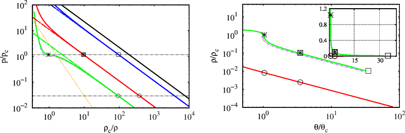
Figure 2: Panel (a): pressure-density diagram (log-log coordinates) for the Van der Waals equation of state. Solid lines: isotherms at different temperatures for the Van der Waals equation of state. Dash-dotted lines: isotherms for the perfect fas equation of state. Dotted line (purple in the electronic version): critical isotherm. Symbols: thermodynamics injection conditions of each simulation, namely Sim A and C (asterisks), Sim B (squares), and Sim D (circles). Panel (b): ${\hat{\rho}}-{\hat{\theta}}$ phase diagram and injection conditions of each simulation, same symbols as in panel (a). Inset: same quantities in linear scale.

Panel (a) of figure 2 provides the pressure-density diagram (log-log coordinates) for the Van der Waals equation of state in reduced variables ${\hat{\theta}}=3/8\left({\hat{p}}+3{\hat{\rho}}^{2}\right)\left(1/{\hat{\rho}}-1/3\right)$ and $\hat{p}=p/p_{c}$, $1/\hat{\rho}=\rho_{c}/\rho$, ${\hat{\theta}}=\theta/\theta_{c}$. The dotted line is the critical isotherm ${\hat{\theta}}=1$. The other solid lines are isotherms at increasing temperature. The dash-dotted lines sketch the corresponding isotherms for the perfect gas equation of state, ${\hat{\theta}}=3{\hat{p}}/\left(8{\hat{\rho}}\right)$. The limit behavior of the perfect gas is achieved when two conditions are met, namely i) ${\hat{p}}\gg 3{\hat{\rho}}^{2}$, with the curve ${\hat{p}}=3{\hat{\rho}}^{2}$ shown as the dash-double-dotted line of slope $-2$, and ii) ${\hat{\rho}}\ll 3$, which is the vertical axis delimiting the plot on the left. Increasing the temperature the perfect gas limit is recovered, uppermost solid line of slope $-1$. Moving along an isotherm the perfect gas limit is reached as well at sufficiently low pressure.

The symbols reported in panel (a) of figure 2 provide the thermodynamic conditions for the simulations considered in the paper. The two asterisks are the working points for core jet and environment (leftmost and rightmost symbol, respectively) for the real gas cases, simulations $A$ and $C$ of Table 1. The two open squares (one of which superimposed to an asterisk) give the corresponding points for the perfect gas simulation, simulation $B$ in the same Table. Both asterisks and open squares are on the same isobar, at slightly supercritical pressure ${\hat{p}}=1.17$. The density ratio for simulations A, C (asterisks) and B (open squares) is the same, $\rho_{core}/\rho_{ext}\simeq 10$. On the two isotherms concerning the real gas conditions (asterisks) two additional working points at a substantially lower pressure, ${\hat{p}}=0.02941$ corresponding to atmospheric pressure for Nitrogen, are denoted by open circles and provide the injection conditions for simulation D. Here the gas behavior can be approximated with the perfect gas law. The temperature ratio for simulation D is the same as that for simulations A and C. Clearly the density ratio is instead much lower, $\rho_{core}/\rho_{ext}\simeq 4$. The ${\hat{\rho}}-{\hat{\theta}}$ phase diagram of the conditions of each simulation is represented in panel (b) of figure 2.

The two constants of the Van der Waals model, $a^{*}=3p^{*}_{c}/\rho_{c}^{*2}$ and $b^{*}=1/\left(3\rho^{*}_{c}\right)$, are determined from the critical pressure and density of Nitrogen. Assuming the value of the universal gas constant, the critical temperature is estimated as $\theta^{*}_{c}=8p^{*}_{c}/\left(3{\cal R}^{*}_{m}\rho^{*}_{c}\right)=97.22\,{\rm K}$ in comparison with $126.2$ pertaining to actual Nitrogen. For our purposes, the Van der Waals model reproduces acceptably well the behavior of Nitrogen with the advantage of having a clear and reasonably simple theoretical derivation. In case better accuracy were needed, alternatives are available, e.g. the Peng-Robinson model.

For the reader’s convenience, it may be worth mentioning what the rationale behind the parameters selection for simulation B is. Simulation B, squares in figure 2, has same pressure and density ratio $\rho^{*}_{core}/\rho^{*}_{env}=10$ of simulation A. The difference is the larger injection temperatures such that Nitrogen behaves as a perfect gas, $\theta^{*}_{core}=529.79\,{\rm K}$ and temperature ratio $\theta^{*}_{env}/\theta^{*}_{core}=\rho^{*}_{core}/\rho^{*}_{env}=10$. At constant pressure, the dynamics of a strongly subsonic perfect gas is substantially controlled by density ratio, Prandtl and Reynolds number. Instead, the parameters entering the description of real gas dynamics also include the distance of the injection conditions from the critical point. Indeed simulation B is designed to achieve the same density ratio and injection pressure of simulation A, using the perfect gas equation of state in the region of the parameter space where Nitrogen recovers the perfect gas behavior.

Indeed, a part from the real vs perfect gas issue, an additional difference exists between simulations A and B, namely the different range of temperatures which affects the transport coefficients. In order to discriminate between the effect of thermodynamic behavior and temperature range, a third simulation, C, has been conceived with same thermodynamic conditions and gas model of simulation A (real gas), now artificially enforcing the Prandtl number of simulation B (perfect gas).

It is important to recall that in all the three cases just considered the density ratio between inner core and external jet plus environment is a large one, $\rho^{*}_{core}/\rho^{*}_{env}=10$. It is worthwhile comparing the results with a fourth simulation, D, where the density ratio is substantially lower due to a lower environment pressure, as for Nitrogen at atmospheric pressure and same injection temperatures of the basic simulation $A$ (real gas), $\theta^{*}_{core}=131.46\,{\rm K}$, $\theta^{*}_{env}/\theta^{*}_{core}\simeq 4$, which results in $\rho^{*}_{core}/\rho^{*}_{env}=4$. This simulation is performed with the Van der Waals equation of state and the actual transport coefficients of Nitrogen in the parameter region where Nitrogen behaves almost like a perfect gas (i.e. the real system could have been accurately approximated with the perfect gas equation of state).

sim A-C	inner jet	outer jet	surrounding environment
$p^{*}$	$p^{*}_{R}$	$p^{*}_{R}$	$p^{*}_{R}$
$\rho^{*}$	$\rho^{*}_{R}$	$0.1\,\rho^{*}_{R}$	$0.1\,\rho^{*}_{R}$
$\theta^{*}$	$\theta^{*}_{R}$	$4\,\theta^{*}_{R}$	$4\,\theta^{*}_{R}$
$(\rho^{*}U^{*}A^{*})_{inj}$	$\rho^{*}_{R}|{\bf u}_{R}^{*}|\pi R^{*2}$	$0.234\,\rho^{*}_{R}|{\bf u}_{R}^{*}|\pi R^{*2}$	–
$(\rho^{*}U^{*2}A^{*})_{inj}$	$\rho^{*}_{R}|{\bf u}_{R}^{*}|^{2}\pi R^{*2}$	$1.296\,\rho^{*}_{R}|{\bf u}_{R}^{*}|^{2}\pi R^{*2}$	–

sim B	inner jet	outer jet	surrounding environment
$p^{*}$	$p^{*}_{R}$	$p^{*}_{R}$	$p^{*}_{R}$
$\rho^{*}$	$\rho^{*}_{R}$	$0.1\,\rho^{*}_{R}$	$0.1\,\rho^{*}_{R}$
$\theta^{*}$	$\theta^{*}_{R}$	$10\,\theta^{*}_{R}$	$10\,\theta^{*}_{R}$
$(\rho^{*}U^{*}A^{*})_{inj}$	$\rho^{*}_{R}|{\bf u}_{R}^{*}|\pi R^{*2}$	$0.234\,\rho^{*}_{R}|{\bf u}_{R}^{*}|\pi R^{*2}$	–
$(\rho^{*}U^{*2}A^{*})_{inj}$	$\rho^{*}_{R}|{\bf u}_{R}^{*}|^{2}\pi R^{*2}$	$1.296\,\rho^{*}_{R}|{\bf u}_{R}^{*}|^{2}\pi R^{*2}$	–

sim D	inner jet	outer jet	surrounding environment
$p^{*}$	$p^{*}_{R}$	$p^{*}_{R}$	$p^{*}_{R}$
$\rho^{*}$	$\rho^{*}_{R}$	$0.25\,\rho^{*}_{R}$	$0.25\,\rho^{*}_{R}$
$\theta^{*}$	$\theta^{*}_{R}$	$4\,\theta^{*}_{R}$	$4\,\theta^{*}_{R}$
$(\rho^{*}U^{*}A^{*})_{inj}$	$\rho^{*}_{R}|{\bf u}_{R}^{*}|\pi R^{*2}$	$0.234\,\rho^{*}_{R}|{\bf u}_{R}^{*}|\pi R^{*2}$	–
$(\rho^{*}U^{*2}A^{*})_{inj}$	$\rho^{*}_{R}|{\bf u}_{R}^{*}|^{2}\pi R^{*2}$	$1.296\,\rho^{*}_{R}|{\bf u}_{R}^{*}|^{2}\pi R^{*2}$	–

Table 1: Thermodynamic and physical conditions at injection and surrounding environment normalized with the reference quantities. Top table: real gas (simulations A-C) where the reference quantities are: $p^{*}_{R}=1.178p^{*}_{c}$, $\rho^{*}_{R}=1.0424\rho^{*}_{c}$ and $\theta^{*}_{R}=1.0417\theta^{*}_{c}$. Middle table: perfect gas (simulation B) with reference quantities: $p^{*}_{R}=1.178p^{*}_{c}$, $\rho^{*}_{R}=0.10424\rho^{*}_{c}$ and $\theta^{*}_{R}=4.198\theta^{*}_{c}$. Bottom table: real gas (simulation D) where the reference quantities are $p^{*}_{R}=0.0294117p^{*}_{c}$, $\rho^{*}_{R}=0.010672\rho^{*}_{c}$ and $\theta^{*}_{R}=1.04\theta^{*}_{c}$; due to low pressure and density the limit of perfect gas behavior is almost reached.

Concerning momentum, in all the four cases the momentum ratio is kept constant at $\rho^{*}_{ext}|{\bf u}^{*}_{ext}|/\left(\rho^{*}_{core}|{\bf u}^{*}_{core}|\right)=0.4$. For the purpose of making equations dimensionless reference conditions are selected as the corresponding core jet features $\rho^{*}_{R}=\rho^{*}_{core},p^{*}_{R}=p^{*}_{core}=p^{*}_{env},|{\bf u}^{*}_{R}|=|{\bf u}^{*}_{core}|$.

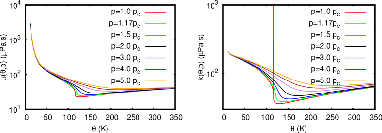
Figure 3: Dependence of Nitrogen viscosity $\mu(\theta,p)$, panel (a), and thermal conductivity $k(\theta,p)$, panel (b), on temperature and pressure. The complete analytical relations are provided in Appendix B.

Table 1 provides detailed information for the different simulations. We stress once more that in cases $A$ and $B$ density and momentum ratios between core and outer stream are the same, $\rho^{*}_{core}/\rho^{*}_{ext}=10$ and $\left(\rho^{*}_{ext}|{\bf u}^{*}_{ext}|\right)/\left(\rho^{*}_{core}|{\bf u}^{*}_{core}|\right)=0.4$. The comparison is aimed at addressing the effects of supercritical injection on jet dynamics and mixing process, at low-Mach number, hence with neglecting acoustic effects. The two simulations mainly differ for the temperatures of core and outer jet. While in the perfect gas case, for given pressure, the density ratio $\rho^{*}_{core}/\rho^{*}_{ext}=10$ results in the temperature ratio $\theta^{*}_{core}/\theta^{*}_{ext}=0.1$, in the real gas case the temperature ratio is $\theta^{*}_{core}/\theta^{*}_{ext}\simeq 0.25$. The bottom panel of Table 1 provides the physical and thermodynamic conditions of simulation D. Here since the temperature ratio $\theta^{*}_{ext}/\theta^{*}_{core}$ matches that of simulation A, the density ratio is much smaller than all the other cases, $\rho^{*}_{core}/\rho^{*}_{ext}=\theta^{*}_{ext}/\theta^{*}_{core}\simeq 4$.

The model is completed with the expressions for dynamic viscosity and thermal diffusivity as a function of pressure and temperature. We use here the relations provided in Ref lemjac, ,

$$\begin{array}[]{cl}\mu^{*}&=\mu^{*0}(\theta^{*})+\mu^{*r}(\tau,\delta)\\ &\\ k^{*}&=k^{*0}(\theta^{*})+k^{*r}(\tau,\delta)+k^{*c}(\tau,\delta)\end{array}$$ (37)

where $\tau=\theta^{*}_{c}/\theta^{*}$ and $\delta^{*}=\rho^{*}/\rho^{*}_{c}$, with $\mu^{*0}$ and $k^{*0}$ the perfect gas viscosity and thermal conductivity, respectively, $\mu^{*r}$ and $k^{*r}$ the so-called residual fluid contributions, and $k^{*c}$ the critical enhancement of thermal conductivity lemjac . Since the effect of the critical condition on viscosity is negligible no critical enhancement is considered. The expressions entering eqs. (37) are explicitly reported in Appendix B with the model constant chosen to reproduce Nitrogen. Figure 3 shows the resulting behavior of viscosity and thermal conductivity as a function of temperature and pressure.

Using the core jet parameters as reference conditions, eqs. (7), the Prandtl number, eq. (II), is $Pr=0.35$ for simulation A (real gas), $Pr=0.6$ for simulation B (high pressure perfect gas case) and C (real gas with transport coefficient matching the high pressure perfect gas case B) and $Pr=0.75$ for simulation D (low pressure case, real gas behaving like a perfect gas). These values are determined through the transport coefficients (37) and the specific heat coefficient (45) evaluated at the respective reference thermodynamic conditions. It is worth stressing that the difference in the Prandtl number between cases A and B/C is substantial.

In all cases buoyancy is neglected since it would have introduced an explicit dependence on the density ratio, thus hampering a fair comparison between the different gas models.

V Results

V.1 Mean fields

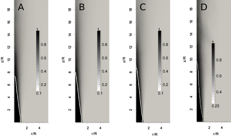
Figure 4: Normalized mean density fields $\rho^{*}/\rho^{*}_{jet}$. From left to right: real gas jet (sim. A), perfect gas jet (sim. B), real gas jet with perfect gas transport properties (sim. C) and real gas jet at low pressure (sim. D), respectively.

As anticipated four simulations are considered. For each of them average fields are extracted by ensemble averaging of about $200$ independent instantaneous configurations separated in time by $0.25R/U_{r}$. Each sample was acquired after the flow reached statistically steady conditions. The typical correlation time $\tau_{c}=0.083R/U_{r}$ is estimated from the autocorrelation of the axial velocity fluctuation $u^{\prime}_{z}(\phi,r,z,t)=u_{z}-\langle u_{z}\rangle$ on the jet axis one diameter downstream of the inlet section ($r=0,z=D$),

$$\tau_{c}=\frac{\displaystyle\int_{0}^{50R/U_{r}}\int_{0}^{50R/U_{r}}u^{\prime}_{z}(\phi,0,D,t)u^{\prime}_{z}(\phi,0,D,t+\tau)dtd\tau}{\displaystyle\int_{0}^{50R/U_{r}}{u^{\prime}_{z}}^{2}(\phi,0,D,t)d\tau}\ .$$

Here and in the following, the subscript $0$ is dropped from the variables, since no confusion may arise and the hydrodynamic pressure $p_{2}$ is never mentioned explicitly.

The dimensionless average density $\rho^{*}/\rho^{*}_{core}$ is illustrated in figure 4 where it ranges from 1 in the jet core to 0.1 in the outer stream for the three density matched simulations including both the two real gas simulations (case A and C) and the perfect gas simulation (case B). The density ranges instead from $1$ (core jet) to $0.25$ in the outer stream for simulation D (low pressure, real gas case) which is temperature matched with the high pressure, real gas simulations A and C. The mixing efficiency may be quantified by the extension of the core region measured, e.g., by the intercept on the jet axis of a selected high-density isoline, $\rho^{*}=0.95\rho_{core}^{*}$ in the present case. The figure shows that the low pressure case (D) exhibits the longest core length.

Concerning the dimensionless temperature $\theta^{*}/\theta^{*}_{ext}$, figure 5, its normalized mean field ranges from 4 in the jet core to 1 in the outer stream for the real gas cases (A and C). For the perfect gas case B the temperature ranges instead from 10 in the jet core to 1 in the outer part. In other words, at fixed density ratio, a higher temperature ratio characterizes the perfect gas case as a consequence of the different equation of state that become crucial in near critical conditions.

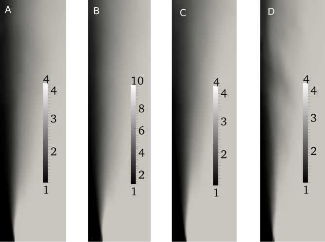
Figure 5: Normalized mean temperature fields $\theta^{*}/\theta^{*}_{ext}$. From left to right: real gas jet (sim. A), perfect gas jet (sim. B), real gas jet with perfect gas transport properties (sim. C) and real gas jet at low pressure (sim. D), respectively.

V.2 Instantaneous fields

The four panels in Figure 6 compare planar cuts of instantaneous axial momentum fields, $\rho u_{z}$, shaded contours. The solid lines denote two density isolevels, namely $\rho=0.9$ and $\rho=0.2$, respectively. In the near field, close to the inlet, typical structures are apparent at the shear layers formed between inner and outer streams where high density contrast occurs between inner and outer jet (cases A, B, and C). They correspond to the finger-like objects observed in the experimental snapshot chetalcoy ; chetalmaybrasmischosc and known to characterize supercritical jets also at moderate Mach numbers. Such structures are much less apparent in the low density ratio case D (atmospheric pressure case). Interestingly they also exist in the high pressure perfect gas jet (B), confirming that they are associated with the high density contrast between inner and outer stream. The structures are similar to the ligaments occurring in the break-up of a liquid jet eggvil . They are formed through a similar kinematic mechanism but are associated with different thermodynamic phenomenologies chetalcoy ; segpol . The liquid (subcritical) jet is characterized by two immiscible phases, liquid and gaseous, with no mutual diffusion. In this case the joint effect of shear and capillary instability promoted by the surface tension acting at the liquid-gas interface induces droplet formation. The external high velocity gas stream stretches the liquid core, forming finger-like structures that elongate until they break-up into droplets due to capillarity eggvil ; bellan . For the cases at high core density (A, B, and C), the density continuously varies from a liquid-like large value in the core to a gas-like low value in the external stream. No truly sharp interface exists however, and consequently no corresponding surface tension. In this context the finger-like structures observed in the corresponding panels of figure 6 are still due to the stretching of the inner core by the faster external stream. However their persistence cannot be ascribed to phase separation, like in the liquid-gas system. Rather they are due to a relatively poor diffusivity of the high density features in the background low density environment. Indeed the essential phenomenology is associated with thermal diffusivity which, at fixed injection pressure, tends to smear out the temperature difference existing between low temperature fluid structures originated in the core and the high temperature surroundings. If the process occurs too slowly with respect to the typical axial velocity, the density structures tend to persist for a significant length beyond the inlet section. This jet dynamics at supercritical conditions is known in literature as jet disintegration royjolseg ; segpol .

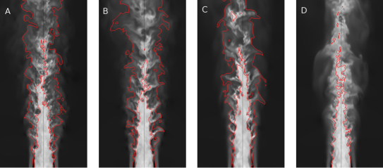
Figure 6: Axial momentum field ($\rho u_{z}$, gray scale contours) with two density isolevels ($\rho=0.9,0.2$, respectively) shown by solid lines. From left to right: case A (real gas, high pressure), case B (perfect gas, high pressure), case C (real gas, with modified transport coefficients) and case D (real gas, low pressure). In the last case the $0.2$ density isoline does not exist.

The concept is better illustrated by manipulating the continuity equation (25) by inserting the expression for the velocity divergence provided by the energy equation (27),

$${\displaystyle\frac{\partial\rho}{\partial t}}+{\bf u}\cdot\nabla\rho=-{\displaystyle\frac{\rho}{Zp}}\frac{1}{RePr}{\bf\nabla\cdot}(k{\bf\nabla}\theta)\left[\frac{1}{\displaystyle{1+\frac{\left(\gamma-2\right)a\rho^{2}}{p\gamma}+\frac{2ab\rho^{3}}{p\gamma}}}\right]\,.$$ (38)

On the basis of this equation, the density adapts along a fluid trajectory due to thermal diffusion that forces the fluid expansion toward thermodynamic equilibrium with the external conditions. As a matter of fact, as the core jet thermodynamic state approaches the critical point, the temperature difference between inner and outer streams keeps on reducing for given density ratio, see the asterisks in comparison with open squares in the right panel of figure 2. Given the injection pressure, the material derivative of the density on the left hand side of the equation can be expressed as $D\rho/Dt=\left({\partial\rho}/{\partial\theta}\right)_{p}D\theta/Dt$, so that the effective Péclet number for the temperature equation, $D\theta/Dt=\left(1/Pe\right)\nabla\cdot\left(k\nabla\theta\right)$, is given by

$$\frac{1}{Pe}=-\left(\frac{\partial\theta}{\partial\rho}\right)_{p}{\displaystyle\frac{\rho}{Zp}}\frac{1}{RePr}\left[\frac{1}{\displaystyle{1+\frac{\left(\gamma-2\right)a\rho^{2}}{p\gamma}+\frac{2ab\rho^{3}}{p\gamma}}}\right]>0\ .$$

The dependence of both Péclet number and dimensionless thermal conductivity $k$ on the local temperature is non-linear and does not easily allow to predict the effective diffusion of the jet in presence of turbulence. It is then worthwhile extracting from the simulation an effective turbulent diffusivity $D_{eff}^{*}$. It is constructed with a transverse diffusion length-scale – in the present case the radius of the inner injection nozzle $R^{*}$ (we recall that the asterisk denote dimensional quantities) – and the convective characteristic time-scale $T^{*}=z_{D}^{*}/|{\bf u}^{*}_{core}|$ corresponding to the time needed by a particle travelling on the axis of the jet to reach the position where mixing between internal and external streams is completed. In practice the mixing length $z_{D}^{*}$ is quantified by the distance from the jet nozzle where the average local density on the axis decreases by a prescribed amount with respect to the injection condition, see the isoline highlighted in figure 4. The turbulent diffusivity follows as

$$D_{eff}^{*}=\frac{{R^{*}}^{2}|{\bf u}^{*}_{core}|}{z_{D}^{*}}$$

providing the expression for the turbulent Péclet number, $Pe_{T}=R^{*}|{\bf u}^{*}_{core}|/D_{eff}^{*}=z_{D}^{*}/R^{*}=z_{D}/R$, in terms of the dimensionless mixing length. The ratio of the molecular, $Pe=\rho^{*}|{\bf u}^{*}_{core}|R^{*}/(k^{*}/c_{p}^{*})$, to the turbulent Péclet number $Pe/Pe_{T}=\rho^{*}D_{eff}^{*}/(k^{*}/c_{p}^{*})$ measures the enhanced diffusion due to turbulence.

As anticipated, in the present case, the dimensionless mixing length $z_{D}^{*}/R^{*}$ is evaluated from the average density field as the position of the intercept of the selected $\rho$-isoline ($\rho^{*}=.95\rho^{*}_{core}$) with the jet axis. For the four cases we find $z^{*}_{D}(A)\simeq 7.4R^{*}$, $z^{*}_{D}(B)\simeq 7.9R^{*}$, $z^{*}_{D}(C)\simeq 8.8R^{*}$, $z^{*}_{D}(D)\simeq 9.8R^{*}$. Dimensional analysis provides a list of parameters upon which $z^{*}_{D}/R^{*}$ may depend, namely

$$\frac{z_{D}^{*}}{R^{*}}=f\left(\frac{R_{1}^{*}}{R^{*}},\frac{R_{2}^{*}}{R_{1}^{*}},\frac{\rho_{core}^{*}}{\rho_{c}^{*}},\frac{\rho_{core}^{*}}{\rho_{ext}^{*}},\frac{p_{env}^{*}}{p_{c}^{*}},\frac{\rho_{core}^{*}|{\bf u}^{*}_{core}|}{\rho_{ext}^{*}|{\bf u}^{*}_{ext}|},Re,Pr\right)\,,$$

where the dependence on the turbulent intensity of the incoming inner stream is accounted for through the Reynolds number. In the cases we address, geometry, momentum ratio ${\rho_{core}^{*}|{\bf u}^{*}_{core}|}/({\rho_{ext}^{*}|{\bf u}^{*}_{ext}|})$, and Reynolds number are held fixed. From the numerical results we find a weak dependence on the pressure ratio $p_{env}^{*}/p_{c}^{*}$, on the Prandtl number $Pr$, and on injection density $\rho_{core}^{*}/\rho_{c}^{*}$ that result in an almost constant $z_{D}^{*}/R^{*}\simeq 7-8$ for the three high pressure cases and a little larger for the lowest pressure $z_{D}^{*}/R^{*}\simeq 9.8$.

Let us now assume that one intends to simplify the system by modelling the high-pressure, real gas injection with the perfect gas model for fixed mass flow rate, i.e. given $\rho_{core}^{*}|{\bf u}^{*}_{core}|$, and for the same injector geometry. Two alternative procedures can be reasonably conceived, namely keeping the same injection density (${\rho^{*}}_{core}^{R}={\rho^{*}}_{core}^{P}$, with the superscript $R$ and $P$ denoting the real and the perfect gas case respectively) or, alternatively, the same temperature (${\theta^{*}}_{core}^{R}={\theta^{*}}_{core}^{P}$). Since $z^{*}_{D}/R^{*}$ is more or less constant, in the first case (same density), where $|{\bf u}^{*}_{core}|^{R}=|{\bf u}^{*}_{core}|^{P}$, the persistence time of the structures $T^{*}=z_{D}^{*}/|{\bf u}^{*}_{core}|$ will be the same for the real gas and for its perfect gas model. In the other case (same temperature), the different injection density $\rho_{core}^{*R}>\rho_{core}^{*P}$ entails a different injection speed resulting in a longer persistence time for the real gas. We observe that, commonly, the injection temperatures are the experimental control parameters, leading to an increased persistence of the real gas coherent structures of density with respect to the perfect gas analogue.

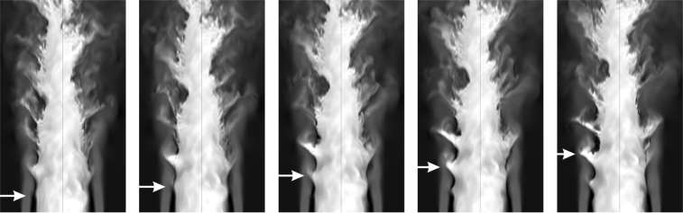
Figure 7: Real gas (Sim A) Instantaneous configurations of the near field of axial momentum. From left to right, consecutive instants of time with a time gap equal to $0.25\,R^{*}/|{\bf u}^{*}_{R}|$. The arrows highlight the evolution of a specific “ligament”.

The dynamics of ligaments formation is addressed in figure 7 by showing five successive configurations of the jet near field. Ligament formation, growth and evolution are clearly visualized by the axial momentum isocontours (see the arrow used to highlight the same structure in the successive stages of development). The wake of the finite thickness trailing edge separating the inner from the outer stream, see the sketch in figure 1, gives rise to the system of Kelvin-Helmholtz vortices apparent in figure 8. They force the internal, slow, and dense gas towards the external, fast, and light stream. The extruded structures are consequently elongated by the high velocity stream to form the ligaments. Panel (a) of figure 8 provides the instantaneous density field on an axial plane, together with the in-plane velocity vectors and three isolevels of a passive scalar injected in the external stream. The contour plot of the passive scalar field is superimposed to the in-plane velocity vectors in the panel (b). The ligament formation is apparently correlated with the Kelvin-Helmholtz vortices, highlighted by the velocity vectors and by the passive scalar isolines. The dense structures protruding from the inner core contribute to slow down the external stream thereby blocking the flow and inducing additional radial motion. It is worthwhile stressing that the dynamics of ligament formation is generic as long as a strong density and velocity contrast exists between the two streams. Indeed, although figure 8 concerns the real gas simulation A, a substantially identical phenomenology is found in all the other two cases with large inner/outer density ratio (B, C). In the fourth case, D, persistent ligaments are not observed and density structures are much less neatly defined due to the small density contrast between the streams.

The most significant difference among the three high density ratio cases is found in the small scale features of the jet, that turn out to be deeply influenced by the thermodynamic behavior of the fluid.

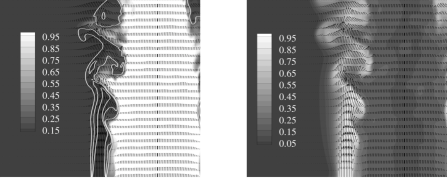
Figure 8: Magnification of the region characterized by the formation of ligaments in the last instantaneous field shown in the rightmost panel of figure 7. Panel (a): instantaneous density field with in-plane velocity vectors. Solid white lines denote three levels of passive scalar injected through the external stream. Panel (b): passive scalar contour with the in-plane velocity vectors.

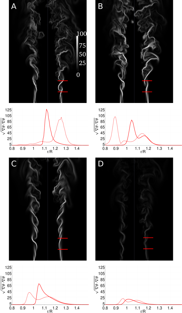
Figure 9: Temperature gradient magnitude $\sqrt{{\bf\nabla}\theta\cdot{\bf\nabla}\theta}$ field. From left to right and from top to bottom: real gas jet (Sim A), perfect gas jet (Sim B), real gas jet with the transport properties of the perfect gas case (Sim C), perfect gas jet matching the temperature ratio of the real gas case (Sim D). The bottom part of each panel report the radial profiles of the temperature gradient magnitude at z=R (solid lines) and z=2R (dashed lines), in the field contour the two axial stations are highlighted with the red segments.

Figure 9 addresses the magnitude of the instantaneous temperature gradients, $\sqrt{{\bf\nabla}\theta\cdot{\bf\nabla}\theta}$. A peculiar aspect is that the temperature gradients have substantially the same order of magnitude for the two real gas cases (top and bottom panel in the left column) and for the perfect gas case (top right panel), despite the temperature difference between inner and outer jet is smaller for the former two cases than it is for the perfect gas case. It follows that the scales at which the temperature gradients occur tend to be smaller in supercritical conditions. In order to make the argument clear, let us consider a dimensional estimate for the temperature gradients, $\sqrt{{\bf\nabla}\theta\cdot{\bf\nabla}\theta}\sim\Delta\Theta/\ell_{\theta}$, where $\Delta\Theta$ is the temperature jump across the interface and $\ell_{\theta}$ is the effective thickness of the instantaneous thermal interface between the high and low temperature regions. Our data show that $\Delta\Theta^{A}/\ell_{\theta}^{A}\simeq\Delta\Theta^{B}/\ell_{\theta}^{B}$. Since $\Delta\Theta^{A}<\Delta\Theta^{B}$, it follows $\ell_{\theta}^{A}<\ell_{\theta}^{B}$, i.e. the thermal thickness for the real gas, supercritical jet is smaller than for the perfect gas case. The statistical characterization of this behavior will be provided in the following section.

According to eq. (29) where $p(t)=const$, the density gradients are associated with the corresponding temperature gradients, $\nabla\rho=\left(\partial\rho(\theta,p)/\partial\theta\right)\nabla\theta$. Here the real gas thermodynamics makes the difference and the singularity near the critical point plays a role, since $\partial\rho(\theta,p_{c})/\partial\theta\rightarrow\infty$ for $\theta\rightarrow\theta_{c}$, where we recall that $p_{c}$ and $\theta_{c}$ are the critical pressure and temperature, respectively. This leads to a further intensification of the density gradients for the real gas near the critical point, with respect to the perfect gas case. Indeed, the dimensional estimate for the density thickness of the interface, $\ell_{\rho}\sim\Delta P/\sqrt{{\bf\nabla}\rho\cdot{\bf\nabla}\rho}$, where $\Delta P$ is the density jump across the interface, is $\ell_{\rho}\sim\ell_{\theta}(\Delta P/\Delta\Theta)/\left(\partial\rho/\partial\theta\right)$ (here the symbol $P$ reads capital $\rho$). This expression shows that the density thickness becomes much thinner than the thermal thickness where the gas gets close to the critical conditions. This behavior of the density gradients can be appreciated in figure 10 that provides the isolevels of the gradient intensity for two instantaneous configurations, corresponding to the real gas and the perfect gas simulation, left and right panel, respectively. Close to the injection section, the density interface is apparently much sharper for the configuration reported on the left. Increasing the distance from the exit, the persistent filamentary structures observed for this case become less evident and weaker in the perfect gas case. Meanwhile, the mixing region becomes increasingly convoluted by small scale, sharply contrasted details which are missing instead at corresponding positions in the right panel. This behavior corresponds to increased turbulent mixing with respect to the perfect gas case.

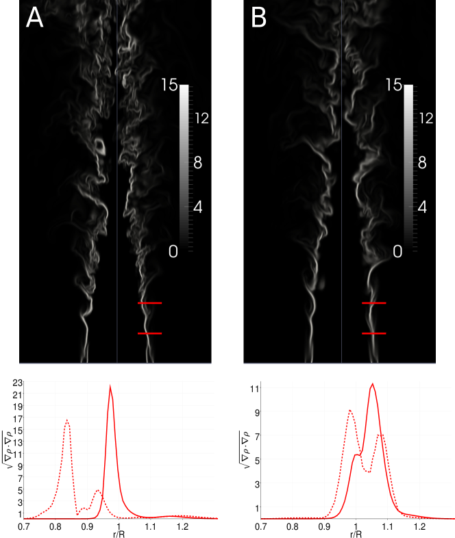
Figure 10: Instantaneous density gradient fields of real gas jet (Sim A) (left top panel) and perfect gas jet (Sim B) (right top panel). The field of simulation C is similar to the simulation A while the density gradients of simulation D are negligible respect to the showed one, since they are omitted. In the bottom panels the radial profiles of the density gradient magnitude at z=R (solid lines) and z=2R (dashed lines) are reported, In the top panels the two axial stations are highlighted with the red segments.

V.3 Statistical analysis

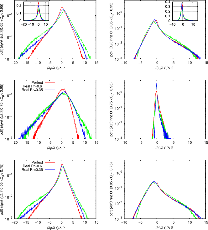
Figure 11: Probability density function of the radial component of the density gradient fluctuation $\partial\rho^{\prime}/\partial r/\Delta P$ (left column, panels a,c,e), and of the temperature gradient fluctuation $\partial\theta^{\prime}/\partial r/\Delta\Theta$ (right column, panels b,d,f). $\Delta P=\rho_{core}-\rho_{ext}$ and $\Delta\Theta=\theta_{core}-\theta_{ext}$ are respectively the density and temperature difference between jet core and external environment. The statistics concerns the region extending two diameters downstream the inlet section $0<z<4R$ and is conditioned to different ranges of the density, namely $0.05<C_{\rho}<0.95$ (top; panels a,b), $0.75<C_{\rho}<0.95$ (middle; panels c,d) and $0.05<C_{\rho}<0.75$ (bottom; panels e,f), where $C_{\rho}=\left(\rho-\rho_{ext}\right)/\Delta P$ is the normalized density ranging from $C_{\rho}=0$ in the external environment to $C_{\rho}=1$ in the jet core.

The previous subsection dealt with the instantaneous configurations of the jets. The conclusions we reached are now better substantiated by quantitatively addressing the related statistics. The statistical analysis is based on the same collection of about two hundred instantaneous fields, separated in time by $0.25\,R^{*}/|{\bf u}^{*}_{R}|$, used for the mean fields.

The panels in the left column of Figure 11 show the probability density function of the radial component of the normalized density fluctuation gradient, $(\partial\rho^{\prime}/\partial r)/\Delta P$, with $\rho^{\prime}=\rho-\langle\rho\rangle$ and $\langle\rho\rangle$ the local mean density. As a matter of fact the density gradient is, on average, almost aligned with the radial direction suggesting that the statistics of $\partial\rho^{\prime}/\partial r$ conveys most of the information on the structure of the instantaneous field. The statistics concerns the region extending two diameters downstream the inlet section ($0\leq z\leq 4R$) and is conditioned to different density ranges, namely $0.05<C_{\rho}<0.95$ (top panel), $0.75<C_{\rho}<0.95$ (middle panel), $0.05<C_{\rho}<0.75$ (bottom panel), with $C_{\rho}=\left(\rho-\rho_{ext}\right)/\Delta P$ the density normalized such that $C_{\rho}=0$ in the external stream and $C_{\rho}=1$ in the core. The panels in the right column of Figure 11 refer to the radial component of the temperature fluctuation gradient, $\partial\theta^{\prime}/\partial r/\Delta\Theta$, with $\theta^{\prime}=\theta-\langle\theta\rangle$ the temperature fluctuation with respect to the mean one $\langle\theta\rangle$ and $\Delta\Theta=\theta_{core}-\theta_{ext}$. Conditioning to density is indeed instrumental to focus the analysis on the instantaneous interface between high density inner core and low density outer stream. This is the region of the phase space where well defined ligaments tend to be formed, see Figure 10. In the three cases (A, real gas; B, perfect gas; C, real gas with artificial transport properties) the pdf $f(\partial\rho^{\prime}/\partial r/\Delta P|0.05\leq C_{\rho}\leq 0.95,0\leq z\leq 4R)$ is significantly skewed towards the negative tail, see top panel on the left and the related inset showing the pdf in logarithmic and linear scale, respectively. The real gas cases show longer tails indicating large intensity events comparatively more frequent than in the perfect gas case. This behavior is quantified by the normalized even moments of the pdf, the so-called hyper-flatness factors of order $n$

$$F_{2n}[\partial\rho^{\prime}/\partial r]=\frac{\langle\left(\partial\rho^{\prime}/\partial r\right)^{2n}\rangle}{\langle\left(\partial\rho^{\prime}/\partial r\right)^{2}\rangle^{n}}\,\qquad\qquad F_{2n}[\partial\theta^{\prime}/\partial r]=\frac{\langle\left(\partial\theta^{\prime}/\partial r\right)^{2n}\rangle}{\langle\left(\partial\theta^{\prime}/\partial r\right)^{2}\rangle^{n}}\,,$$ (39)

see the data reported in Table 2. Values of the hyper-flatness exceeding the reference values for a Gaussian distribution, $F_{2n}^{G}=3,15,105$ for $n=2,3,4$, signal the existence of an intermittent behavior, where phases of relatively weak gradients are alternated with the presence of relatively rare but intense events. In our system the origin of the intermittency is related to the ligaments that invade regions of relatively smooth density variation.

	n=2	n=3	n=4
sim. A	7.2	110.	2327.
sim. B	6.4	91.	1930.
sim. C	5.1	49.	624.
Gauss	3.0	15.	105.

	n=2	n=3	n=4
sim. A	9.0	172.	4464.
sim. B	8.1	134.	2990.
sim. C	6.0	72.	1151.
Gauss	3.0	15.	105.

Table 2: Hyper-flatness, $F_{2n}\left[\partial\cdot^{\prime}/\partial r\right]$, of the probability distribution reported in the top panels of figure 11. Left table: radial component of density gradient fluctuations; right table: radial component of temperature gradient fluctuations.

Given the relationship between temperature and density gradients, $\partial\theta^{\prime}/\partial r=\left(\partial\theta/\partial\rho\right)\partial\rho^{\prime}/\partial r$, the overall shape of the temperature pdf is grossly speaking specular with respect to that of density since $\partial\theta/\partial\rho<0$. Interestingly, the three temperature gradient pdfs for the two real gas and the perfect gas case are substantially identical, confirming the impression gained from inspecting the instantaneous field, see Figure 9. We stress that conditioning with respect to density is used in the two top panels at the only purpose of removing from the analysis the events of vanishing gradients occurring in the external region and in the inner jet core that would otherwise outnumber the comparatively less numerous events belonging to the physically significant interface between inner and outer stream.

In order to focus on the large density features, the middle panels of Figure 11 show the fluctuation gradient pdf conditioned to the high density range $0.75<C_{\rho}<0.95$. It is apparent that the origin of the intermittent behavior of the density gradients (left panel) is mostly related to features associated with large density. The pdf shows exponential tails which are definitely longer in the two real gas cases. Conversely, the temperature gradients conditioned to the same density range (right panel) are characterized by a comparatively narrower distribution, indicating that the structures which support the density gradients have almost deterministic temperature gradients, $\partial\theta/\partial r\simeq\partial\langle\theta\rangle/\partial r$, as follows from observing that $\partial\theta^{\prime}/\partial r\simeq 0$. Considered that $\partial\langle\theta\rangle/\partial r=\langle\partial\theta/\partial\rho\,\partial\rho/\partial r\rangle$, since $\partial\rho/\partial\theta$ is large for the near critical gas, it follows that the high density features supporting the density gradients are almost isothermal in the real gas cases.

The bottom panels of Figure 11 concern the complementary density range $0.05<C_{\rho}<0.75$. Apparently the most significant fluctuations of the temperature gradient (left panel) occur in this region of the phase space. The intermittency of the temperature gradient is significant, implying that, locally, a large temperature difference occurs, with relatively low temperature regions getting close to high temperature ones. Clearly, this induces strong density gradients, giving reason of the non-negligible density-gradient intermittency found also in this complementary density range.

The density gradient is strictly related to the thickness of the interface between the high-density core and the low-density external stream. Indeed the high density gradients that characterize the real gas jets suggest that the interface is thinner for the real gas than for the perfect gas. The interface thickness can be estimated as the inverse of the normalized density gradient module $\delta_{\rho}=\Delta P/\left|\nabla\rho\right|$.

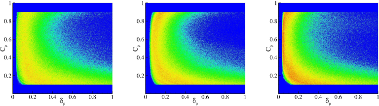
Figure 12: Joint probability density function, $f(\delta_{\rho},C_{\rho})$, of density interface thickness $\delta_{\rho}=\Delta P/\left|\nabla\rho\right|$ and normalized density $C_{\rho}$, in the region one diameter downstream the jet inlet. From left to right: real gas jet (panel a), perfect gas jet (panel b) and real gas jet with perfect gas transport features (panel c).

Figure 12 provides the joint probability density function, $f(\delta_{\rho},C_{\rho})$, of interface thickness $\delta_{\rho}$ and normalized density $C_{\rho}$, where the real gas case A is reported on the panel (a), the perfect gas case B in the panel (b), and the real gas case with perfect gas transport coefficients C in the panel (c). The statistics concern the same region of the flow domain already considered in the pdfs of figure 11 and are conditioned to a density interval ranging from $C_{\rho}=0.9$ to $C_{\rho}=0.1$.

In order to understand the different roles played by the equation of state and by the transport coefficients it is worth first comparing real and perfect gas cases with identical transport coefficients, cases B and C reported in the middle and right-most panel of the figure, respectively. Apparently as the density increases ($C\rho$), the interface thickness decreases for both cases. In comparison with the perfect gas case, at given normalized density, the pdf of the interface thickness is much more peaked at small values for the reals gas case. A further feature to be noted is that, at large density, the peak of the pdf moves toward slightly larger scales for the perfect gas case, implying an increased diffusion of high density features. On the contrary the pdf peak remains centered on the smallest scales for the real gas. This behavior is explained by looking at the isobars in the density-temperature diagram provided in figure 2. The injection states for cases B and C are denoted with the squares and the asterisks, respectively, reported on the same isobar (green curve). Apparently, huge density difference take place at almost constant temperature for case C (real gas), see also the inset with the isobars plotted in linear scale. On the contrary for case B density changes are almost uniformly distributed along the temperature range. Since diffusion effects are determined by the temperature field, eq. (38), it follows that density structures are more diffusive for case B, where they are always associated with significant temperature differences. The comparatively smaller diffusion taking place in the real gas explains the statistically smaller interface thickness observed in the scatter plots shown in the panel (c) of figure 12 in comparison with that shown in the panel (b). The effect is observed at all values of density a part from the smallest range farther from the critical condition, where the isobar gets closer to the behavior of the perfect gas.

When recovering the actual transport coefficients of the real gas (case A), panel (a) of figure 12, the typical scales of the density gradients increase significantly with respect to the artificial case C (real gas with perfect gas transport coefficients). The effect is qualitatively explained by comparing the behavior of the thermal diffusivity $\lambda$ for the real gas shown in the right panel of figure 3, see Appendix B, with the Sutherland law shown as a dashed line in the same figure. Clearly the diffusivity is enhanced, hence the increased scale for the density gradients.

In conclusion, the coherent structures of high density observed as a consequence of the high density and momentum contrast between inner and outer stream are characterized by a sharp interface of separation with the background low density environment. The instantaneous interface is extremely sharp for the real gas (Van der Waals equation of state), although it is partially smeared by the increased thermal diffusivity occurring near the critical point. Such features of coherent density and their sharp interface are responsible for the highly intermittent statistical behavior observed for the density gradients.

VI Final Remarks

The low Mach number asymptotic expansion of the Navier-Stokes equations, originally derived by Majda & Sethian for perfect gas flows in reactive conditions, was here extended to a generic real gas equation of state to deal with fluids in near critical conditions. The resulting formulation allowed the detailed analysis of the turbulent mixing of slightly supercritical fluids at vanishing Mach number through accurate and efficient Direct Numerical Simulations of a coaxial jet of a single component Van der Waals fluid. When slightly supercritical streams are mixed at large Reynolds number, turbulence and real-gas effects combine and have been shown to produce peculiar effects.

Elongated finger-like structures, the so-called “ligaments”, similar to those classically observed in the break-up of liquid jets, are found in the simulations. These structures have been well documented also in supercritical injection experiments and numerical simulation at moderately high Mach number and differ from those characterizing liquid jets which eventually break up in droplets. The supercritical ligaments, once formed, diffuse to eventually disappear altogether. The ligaments are originated by the joint effect of a high density contrast between inner and outer stream in combination with the strong shear layer generated at the interface between the slower inner jet and the outer faster stream. The high velocity ratio of the shear layer promotes the formation of the classical Kelvin-Helmholtz instability with rolling vortices. Finger-shaped high density protrusions are extruded by these vortices in the low density high speed stream where they are elongated well inside the external environment thereby generating the ligaments. It is worth emphasizing that this mechanism operates in all the cases where a high density contrast exists, irrespective of the thermodynamic model. The main difference between Van der Waals and perfect gas jets mostly resides in the small-scale features of the ligaments. In comparison with the perfect gas model, the dense gas case shows much steeper density gradients and a thinner interface between the high- and low-density streams. Instead temperature gradients behave much more similarly in the two cases, despite the fact that the bulk temperature differences are smaller in the dense gas case, for given density contrast. In other words, turbulent mixing in dense gases is associated with smaller scales than in perfect gases in order to balance the smaller temperature jump occurring at near critical conditions for given density contrast between the mixing streams. The steep density gradients near the critical point are indeed associated with the critical point singularity that controls the spatial scales of the density variations.

The statistical signature of this phenomenology is found in the intermittency of the density field, as evaluated by the hyper-flatness of the density gradient pdf. Indeed the increased intermittency in real gas mixing is related to the occurrence of the mentioned ligamentary structures characterized by an extremely sharp interface separating high and low density streams. The picture is reinforced after looking at the large density gradient fluctuations that take place in correlation with high density regions, thermodynamically closer to the critical state. Typically, the ligaments are almost isothermal structures with small temperature differences with the local environment. This behavior is understood after considering that fluid particles at near critical conditions may assume significantly different densities with almost identical temperatures as a consequence of the aforementioned critical point singularity. Overall, the much smaller local interface thickness for the near critical gas may have significant consequences for the numerical simulation of this kind of flows.

As a final remark, we like to stress that the features that have been observed in connection with the Wan der Waals model for the gas are expected to hold also for other thermodynamic model of dense gases (e.g. the Peng-Robinson model), that in certain cases may provide a better description of a real gas.

The intermittent behavior promoted by the ligaments in combination with the sharp interface separating high and low density regions is a crucial feature to be modeled in view of increasing the predictive performances of coarse-grained descriptions like Large-Eddy-Simulation. The formulation here introduced could indeed represent a solid framework to develop appropriate sub-grid models to deal with turbulent diffusion processes in high-Reynolds-number technological applications involving supercritical fluids.

Appendix A Van der Waals and Peng-Robinson equation of state

Thermal properties of polyatomic gases are affected by quantum effects that emerge already at ordinary thermodynamic conditions. In addition, when the density is sufficiently high, molecule-molecule interaction become significant giving rise to the so-called real-gas effects. All this information is gathered in the expression for the Helmholtz free-energy as a function of temperature, volume and molecule number.

A.1 The Van der Waals model

The simplest model endowed with all these features is a diatomic Van der Waals gas, whose Helmholtz free energy $f$ can be derived from quantum statistical mechanics considerationszhu ,

$$f ={\cal R}n\theta\ln{\left[\frac{\left(1-e^{-\frac{\tau}{\theta}}\right)}{C(n)\left(V-b\right)\theta^{5/2}}\right]}-\frac{a}{V}+{\cal R}n\frac{\tau}{2}$$ (40)

where $C(n)=8\pi^{2}n\iota{\cal R}^{5/2}\sqrt{2\pi m}/\left(\hbar^{5}N_{A}^{3/2}\right)$ with $\iota$ and $m$ the moment of inertia and the mass of the molecule, ${\cal R}$ the universal gas constant, $\hbar=h/(2\pi)$ with $h$ the Planck’s constant, $N_{A}$ the Avogadro’s number, $n=N/N_{A}$ the number of moles, $N$ the number of gas molecules, $\tau=\hbar\zeta N_{A}/{\cal R}$ where $\zeta$ is the fundamental vibrational frequency of the molecule. In the expression for the free-energy two additional constant appear, $a$ and $b$ related to the intermolecular forces and to the excluded volume, respectively.

The pressure equation of state follows as

$$p=-\left.\frac{\partial f}{\partial V}\right|_{\theta,N}=\frac{{\cal R}_{m}\theta\rho}{1-b^{\prime}\rho}-a^{\prime}\rho^{2}\,,$$ (41)

where $a^{\prime}=a/(n{\cal W})^{2}$ and $b^{\prime}=b/(n{\cal W})$ with $\cal W$ the molar mass respectively, and ${\cal R}_{m}={\cal R}/{\cal W}$. The entropy is

$${\cal S}=-\left.\frac{\partial f}{\partial\theta}\right|_{V,N} =\frac{5}{2}{\cal R}n\left(\ln{\theta}+1\right)+{\cal R}n\ln{\left[\frac{C(n)\left(V-b\right)}{\left(1-e^{-\frac{\tau}{\theta}}\right)}\right]}+\frac{{\cal R}n\tau}{\left(e^{\tau/\theta}-1\right)\theta}\,,$$ (42)

which yields the internal energy

$$U=F+\theta S=\frac{5}{2}{\cal R}n\theta-\frac{a}{V}+{\cal R}n\tau\left(\frac{1}{2}-\frac{1}{e^{\tau/\theta}-1}\right)\ .$$ (43)

Hence the heat capacity at constant pressure and volume can be calculated from the entropy by means the known thermodynamic relations,

$$c_{v} =\theta\left.\frac{\partial\cal S}{\partial\theta}\right|_{V,N}=\frac{5}{2}{\cal R}n+{\cal R}n\frac{\tau^{2}}{\left(e^{\tau/\theta}-1\right)^{2}\theta^{2}}$$ (44)

$$c_{p} =c_{v}+\theta\left.\frac{\partial p}{\partial\theta}\right|_{V,N}\left.\frac{\partial V}{\partial\theta}\right|_{p,N}=c_{v}+\theta\frac{{\cal R}^{2}n^{2}}{\left(V-b\right)\left(p-a/V^{2}+2ba/V^{3}\right)}\ .$$ (45)

The ideal gas is recovered by setting $a=b=0$, with $\tau=0$ recovering constant, temperature-independent thermal properties. Relations (41), (44) and (45) can be re-expressed as

$$p =\frac{{\cal R}_{m}\theta\rho}{1-b^{\prime}\rho}-a^{\prime}\rho^{2}\,,$$ (46)

$$c_{v}^{\prime} =\frac{c_{v}}{n\cal W}=\frac{5}{2}{\cal R}_{m}+{\cal R}_{m}\frac{\tau^{2}}{\left(e^{\tau/\theta}-1\right)^{2}\theta^{2}}\,,$$ (47)

$$c_{p}^{\prime} =\frac{c_{p}}{n\cal W}=c_{v}^{\prime}+{\cal R}_{m}\frac{{\cal R}_{m}\rho\theta}{\left(1-b^{\prime}\rho\right)\left(p-a^{\prime}\rho^{2}+2b^{\prime}a^{\prime}\rho^{3}\right)}\,,$$ (48)

where $c_{v}^{\prime}=c_{v}/(n{\cal W})$ and $c_{p}^{\prime}=c_{p}/(n{\cal W})$ are the heat capacity coefficients per mass unit.

A.2 The Peng-Robison model

In many circumstances the Van der Waals model is not suffuciently accurate, and should be substituted by alternative thermodynamic models. As an example, the pressure equation for the Peng-Robinson model, penrob , reads

$$p=\frac{k_{B}N\theta}{V-b}-\frac{a\alpha(\theta)}{V+2\,b\,V-b^{2}}\,,$$ (49)

where $V$ is the volume and $a$, $b$ and $\alpha(\theta)$ can be expressed as a function of the critical thermodynamic variables and of what is called the acentric factor $\omega$,

$$a =\frac{0.457235N^{2}k_{B}^{2}\theta_{c}^{2}}{p_{c}}$$

$$b =\frac{0.077796Nk_{B}\theta_{c}}{p_{c}}$$

$$\alpha =\left[1+\kappa\left(1-\theta_{R}^{0.5}\right)\right]^{2}\ ,$$

with $\theta_{R}={\theta}/{\theta_{c}}$ and $\kappa=0.37464+1.54226\,\omega-0.26992\,\omega^{2}$. Considering the relation $p=-(\partial f/\partial V)_{\theta,N}$, the Helmholtz free-energy $f$ associated with the equation of state (49) is obtained by straightforward integration,

$$f=-k_{B}\theta\ln{{\cal Z}}=-k_{B}\theta N\,\int{\frac{1}{V-b}dV}+a\,\alpha(\theta)\int{\frac{1}{V+2\,b\,V-b^{2}}dV}+A(\theta,N)\,,$$ (50)

where $A(\theta,N)$ is the integration constant which depends only on temperature and particle number. The result is

$$f=-k_{B}\theta N\ln{\left|V-b\right|}+\frac{a\alpha(\theta)}{2\sqrt{2}\,b}\ln{\left|\frac{V-\left(\sqrt{2}-1\right)\,b}{V+\left(\sqrt{2}+1\right)\,b}\right|}+A(\theta,N)\,.$$ (51)

The integration constant $A(\theta,N)$ may be evaluated considering that in the limit $V\rightarrow\infty$ for fixed temperature and particle number both the Peng-Robinson and the Van der Waals models should approach the same limit. In other words, in the limit, equations (40) and (51) must eventually coincide, providing by comparison the expression for $A$

$$A(\theta,N)=-\frac{5}{2}k_{B}\theta N\ln{\theta}+k_{B}N\frac{\tau}{2}+k_{B}\theta N\,\ln{\left(1-e^{-\frac{\tau}{\theta}}\right)}-k_{B}\theta N\ln{\left(\frac{8}{\hbar^{5}}\pi^{2}N\iota k_{B}^{5/2}\sqrt{2\pi m}\right)}\,.$$

Once $A$ is found, all the relevant thermodynamic quantities are accessible from the Helmholtz free-energy that reads

$$f= {\cal R}n\theta\ln{\left|V-b\right|}-\frac{a\alpha(\theta)}{\,2\sqrt{2}\,b}\ln{\left|\frac{V-\left(\sqrt{2}-1\right)\,b}{V+\left(\sqrt{2}+1\right)\,b}\right|}$$

$$+ \frac{5}{2}{\cal R}n\theta\ln{\theta}-{\cal R}n\frac{\tau}{2}-{\cal R}n\theta\,\ln{\left(1-e^{-\frac{\tau}{\theta}}\right)}+{\cal R}n\theta\ln{\left(\frac{8}{\hbar^{5}}\pi^{2}N\iota k_{B}^{5/2}\sqrt{2\pi m}\right)}\,.$$ (52)

Appendix B Transport coefficients.

The dynamic viscosity and thermal conductivity are evaluated, see Ref lemjac, , considering the dilute gas contribution, $\mu^{0}$ and $k^{0}$, the residual fluid contribution, $\mu^{r}$ and $k^{r}$, and the critical state contribution, $k^{c}$. The critical state enhancement can be neglected for the dynamic viscosity.

For the viscosity the dilute gas contribution is given by

$$\mu^{0}(\theta)=\frac{0.0266958\sqrt{{\cal W}\theta}}{\sigma^{2}\Omega(\bar{\theta})}\,,$$ (53)

where $\sigma$ is the Lennard-Jones size parameter equal to $\sigma=0.3656\,{\rm nm}$ for the Nitrogen. $\Omega$ is the collisional integral

$$\Omega(\bar{\theta})=\exp{\left(\sum_{i=0}^{4}b_{i}\left[\ln(\bar{\theta})\right]^{i}\right)}\,,$$ (54)

where $\bar{\theta}=\theta/(\varepsilon/k)$ and $\varepsilon/k$ is the Lennard-Jones energy parameter equal to $\varepsilon/k=98.94K$ for the Nitrogen. $b_{i}$ are fitting coefficient provided in Ref lemjac, , and are reported in table 3.

$i$	$b_{i}$
$0$	$0.431$
$1$	$-0.4623$
$2$	$0.08406$
$3$	$0.005341$
$4$	$-0.00331$

Table 3: Fitting coefficients of the Collision integral for the dilute gas viscosity provided in lemjac .

The residual contribution to the dynamic viscosity yields

$$\mu^{r}(\tau,\delta)=\sum_{i=1}^{n}N_{i}\tau^{t_{i}}\delta^{d_{i}}\exp{\left(-\gamma_{i}\delta^{l_{i}}\right)}\,,$$ (55)

where $\tau$ and $\delta$ are the ratios $\tau=\theta_{c}/\theta$ and $\delta=\rho/\rho_{c}$, respectively, while the coefficients $N_{i}$, $t_{i}$, $d_{i}$, $l_{i}$ and $\gamma_{i}$ are reported in table 4.

$i$	$N_{i}$	$t_{i}$	$d_{i}$	$l_{i}$	$\gamma_{i}$
$1$	$10.72$	$0.1$	$2$	$0$	$0$
$2$	$0.03989$	$0.25$	$10$	$1$	$1$
$3$	$0.001208$	$3.2$	$12$	$1$	$1$
$4$	$-7.402$	$0.9$	$2$	$2$	$1$
$5$	$4.620$	$0.3$	$1$	$3$	$1$

Table 4: Coefficients and exponent of the residual viscosity equation.

The dynamic viscosity is obtained by the sum of the two contribution obtaning the viscosity in $\mu Pa\cdot s$. The model for the thermal conductivity, espressed in $mW/(m\cdot K)$, is composed of three contribution. The first one is the dilute gas contribution,

$$k^{0}=N_{1}\left[\frac{\mu^{0}(\theta)}{1\mu Pa\cdot s}\right]+N_{2}\tau^{t_{2}}+N_{3}\tau^{t_{3}}\,.$$ (56)

The second contribution to the thermal conductivity equation is the residual one,

$$k^{r}=\sum_{i=4}^{n}N_{i}\tau^{t_{i}}\delta_{d_{i}}exp{\left(-\gamma_{i}\delta^{l_{i}}\right)}\,.$$ (57)

The third contribution dealing with the critical state correction reads

$$k^{c}=\rho c_{p}\frac{k_{B}R_{0}\theta}{6\pi\xi\mu(\theta,\rho)}\left(\tilde{\Omega}-\tilde{\Omega}_{0}\right)$$ (58)

where

$$\tilde{\Omega} =\frac{2}{\pi}\left[\left(\frac{c_{p}-c_{v}}{c_{p}}\right)\tan^{-1}\left({\frac{\xi}{q_{D}}}\right)+\left(\frac{c_{v}}{c_{p}}\right)\left(\frac{\xi}{q_{D}}\right)\right]$$ (59)

$$\tilde{\Omega}_{0} =\frac{2}{\pi}\left\{1-\exp{\left[\frac{-1}{(\xi/q_{D})^{-1}+(\xi/q_{D})^{2}/3(\rho_{c}/\rho)^{2}}\right]}\right\}$$ (60)

$$\xi=\xi_{0}\left[\frac{\tilde{\chi}(\theta,\rho)-\tilde{\chi}(\theta_{ref},\rho)\theta_{ref}/\theta}{\Gamma}\right]^{\nu/\gamma}$$ (61)

$$\tilde{\chi}(\theta,\rho)=\frac{p_{c}\rho}{\rho_{c}^{2}}\left.\frac{\partial\rho}{\partial p}\right|_{\theta}\ .$$ (62)

The coefficient and exponents of these equations are summarized in table 5, while the other relevant parameters are the Boltzmann’s constant $k_{B}=1.380658\cdot 10^{-23}J/K$, the constants $R_{0}=1.01$, $\nu=0.63$ and $\gamma=1.2415$. Finally a few other constants depend on the specific gas and data fitting on Nitrogen yields $q_{D}=0.4nm$, $\xi_{0}=0.17nm$ and $\Gamma=0.055$. The reference temperature $\theta_{ref}$ is twice the critical temperature, and, in addition, $k_{c}$ should be set to zero when the term in the bracket of equation (61) is negative.

$i$	$N_{i}$	$t_{i}$	$d_{i}$	$l_{i}$	$\gamma_{i}$
$1$	$1.511$
$2$	$2.117$	$-1.0$
$3$	$-3.332$	$-0.7$
$4$	$8.862$	$0.0$	$1$	$0$	$0$
$5$	$31.11$	$0.03$	$2$	$0$	$0$
$6$	$-73.13$	$0.2$	$3$	$1$	$1$
$7$	$20.03$	$0.8$	$4$	$2$	$1$
$8$	$-0.7096$	$0.6$	$8$	$2$	$1$
$9$	$0.2672$	$1.9$	$10$	$2$	$1$

Table 5: Coefficients and exponents of the residual thermal conductivity equation.

Appendix C Thermal form of energy equation for a general EOS

For the reader’s convenience, the calculations needed to obtain the temperature equation for a generic equation of state, eq. (20), are here explicitly reported. The differential of the internal energy as a function of temperature $\theta^{*}$ and density $\rho^{*}$, $u^{*}=u(\theta^{*},\rho^{*})$, is,

$$du^{*}=\left.{\frac{\partial u^{*}}{\partial\theta^{*}}}\right|_{\rho^{*}}d\theta^{*}+\left.\frac{\partial u^{*}}{\partial\rho^{*}}\right|_{\theta^{*}}d\rho^{*}=c_{v}^{*}d\theta^{*}+\left.\frac{\partial u^{*}}{\partial\rho^{*}}\right|_{\theta^{*}}d\rho^{*}\,,$$ (63)

with $c_{v}^{*}=\left.{\partial u^{*}}/{\partial\theta^{*}}\right|_{v^{*}}=\left.{\partial u^{*}}/{\partial\theta^{*}}\right|_{\rho^{*}}$ and $v^{*}=1/\rho^{*}$ the specific volume. Since $d\rho^{*}=\rho^{*2}dv^{*}$, it follows

$$\left.\frac{\partial u^{*}}{\partial\rho^{*}}\right|_{\theta^{*}}d\rho^{*}=-\frac{1}{\rho^{*2}}\left.\frac{\partial u^{*}}{\partial v^{*}}\right|_{\theta^{*}}d\rho^{*}\,.$$ (64)

Combining equations (64) and (63), the material derivative of the internal energy follows as

$$\frac{Du^{*}}{Dt^{*}}=c_{v}^{*}\frac{D\theta^{*}}{Dt^{*}}-\frac{1}{\rho^{*2}}\left.\frac{\partial u^{*}}{\partial v^{*}}\right|_{\theta^{*}}\frac{D\rho^{*}}{Dt^{*}}\,,$$ (65)

which, using the continuity equation, ${1}/{\rho^{*}}{D\rho^{*}/Dt}=-{\bf\nabla}^{\,*}\cdot{\bf u^{*}}$, becomes

$$\frac{Du^{*}}{Dt^{*}}=c_{v}^{*}\frac{D\theta^{*}}{Dt^{*}}+\frac{1}{\rho^{*}}\left.\frac{\partial u^{*}}{\partial v^{*}}\right|_{\theta^{*}}{\bf\nabla}^{\,*}\cdot{\bf u}^{*}=c_{v}^{*}\frac{D\theta^{*}}{Dt^{*}}+v^{*}\left.\frac{\partial u^{*}}{\partial v^{*}}\right|_{\theta^{*}}{\bf\nabla}^{\,*}\cdot{\bf u^{*}}\,.$$ (66)

Inserting eq. (66) in the internal energy equation (3) leads to

$$\rho^{*}c_{v}^{*}\frac{D\theta^{*}}{Dt^{*}}=-\left(p^{*}+\left.\frac{\partial u^{*}}{\partial v^{*}}\right|_{\theta^{*}}\right)\,{\bf\nabla}^{\,*}\cdot{\bf u^{*}}+{\bf\Sigma^{*}}:{\bf\nabla}^{\,*}{\bf u}^{*}+{\bf\nabla}^{\,*}\cdot\left(k^{*}{\bf\nabla}^{\,*}\theta^{*}\right)\,.$$ (67)

The first term on the right hand side of this equation can be rearranged starting from the fundamental thermodynamic relation $du^{*}=\theta^{*}ds^{*}-p^{*}dv^{*}$, where the specific entropy can be expressed as a function of temperature and specific volume $s^{*}=s(\theta^{*},v^{*})$,

$$du^{*} =\theta^{*}\left(\left.\frac{\partial s^{*}}{\partial\theta^{*}}\right|_{v^{*}}d\theta^{*}+\left.\frac{\partial s^{*}}{\partial v^{*}}\right|_{\theta^{*}}dv^{*}\right)-p^{*}dv^{*}$$ (68)

$$=\left(-p^{*}+\theta^{*}\,\left.\frac{\partial s^{*}}{\partial v^{*}}\right|_{\theta^{*}}\right)dv^{*}+\theta^{*}\,\left.\frac{\partial s^{*}}{\partial\theta^{*}}\right|_{v^{*}}d\theta^{*}\ .$$ (69)

Since the specific entropy $-s^{*}$ is the first derivative of the Helmholtz specific free energy $f^{*}$ with respect to the temperature, one of the Maxwell’s relations yieds

$$\left.\frac{\partial s^{*}}{\partial v^{*}}\right|_{\theta^{*}}=-\frac{\partial^{2}f^{*}}{\left.\partial\theta^{*}\right|_{v^{*}}\left.\partial v^{*}\right|_{\theta^{*}}}=\left.\frac{\partial p^{*}}{\partial\theta^{*}}\right|_{v^{*}}$$ (70)

where $p^{*}=-\left.{\partial f^{*}}/{\partial v^{*}}\right|_{\theta^{*}}$. Merging equations (69) and (70), brings to the general identity

$$\left.\frac{\partial u^{*}}{\partial v^{*}}\right|_{\theta^{*}}=-p^{*}+\theta^{*}\left.\frac{\partial s^{*}}{\partial v^{*}}\right|_{\theta^{*}}=-p^{*}+\theta^{*}\left.\frac{\partial p^{*}}{\partial\theta^{*}}\right|_{v^{*}}\,.$$ (71)

Inserting the above expression in the specific energy equation (67), yields the required equation for the temperature field,

$$\rho^{*}c_{v}^{*}\frac{D\theta^{*}}{Dt^{*}}=-\theta^{*}\left.\frac{\partial p^{*}}{\partial\theta^{*}}\right|_{v^{*}}\,{\bf\nabla}^{\,*}\cdot{\bf u}^{*}+{\bf\Sigma^{*}}:{\bf\nabla}^{\,*}{\bf u}^{*}+{\bf\nabla}^{\,*}\cdot\left(k^{*}{\bf\nabla}^{\,*}\theta^{*}\right)$$ (72)

which is indeed the dimensional counterpart of the dimensionless equation reported in the main text as eq. (10).

References

- (1) M.V. Palmer and S.S.T. Ting, “Applications for supercritical fluid technology in food processing,” Food chemistry 52, 345–352 (1995).
- (2) M. Perrut, “Supercritical fluid applications: Industrial developments and economic issues,” Industrial & engineering chemistry research 39, 4531–4535 (2000).
- (3) J. Fages, H. Lochard, J.J. Letourneau, M. Sauceau, and E. Rodier, “Particle generation for pharmaceutical applications using supercritical fluid technology,” Powder Technology 141, 219–226 (2004).
- (4) G. Brunner, “Applications of supercritical fluids,” Annual Review of Chemical and Biomolecular Engineering 1, 321–342 (2010).
- (5) L. Cheng, G. Ribatski, and J.R. Thome, “Analysis of supercritical CO2 cooling in macro- and micro-channels,” International Journal of Refrigeration 31, 1301–1316 (Dec. 2008), ISSN 01407007.
- (6) A. Checinska, I.A. Fruth, T.L. Green, R.L. Crawford, and A.J. Paszczynski, “Sterilization of biological pathogens using supercritical fluid carbon dioxide containing water and hydrogen peroxide,” Journal of microbiological methods 87, 70–75 (2011).
- (7) G.L. Weibel and C.K. Ober, “An overview of supercritical co< sub> 2</sub> applications in microelectronics processing,” Microelectronic Engineering 65, 145–152 (2003).
- (8) J.W. King and G.R. List, Supercritical fluid technology in oil and lipid chemistry (The American Oil Chemists Society, 1996).
- (9) J.A. Mendiola, M. Herrero, M. Castro-Puyana, and E. Ibáñez, “Supercritical fluid extraction,” Natural Product Extraction: Principles and Applications 21, 196 (2013).
- (10) B. Chehroudi, D. Talley, and E. Coy, “Visual characteristics and initial growth rates of round cryogenic jets at subcritical and supercritical pressures,” Physics of Fluids 14, 850 (2002).
- (11) C. Segal and S. a. Polikhov, “Subcritical to supercritical mixing,” Physics of Fluids 20, 052101 (2008), ISSN 10706631.
- (12) A. Roy, C. Joly, and C. Segal, “Disintegrating supercritical jets in a subcritical environment,” Journal of Fluid Mechanics 717, 193–202 (Feb. 2013), ISSN 0022-1120.
- (13) W. Mayer, J. Telaar, R. Braham, G. Schneider, and J. Hussong, “Raman measurements of cryogenic injection at supercritical pressure,” Heat and Mass Transfer 39, 709 (2003).
- (14) W. Mayer, A. Schik, C. Schweitzer, and M. Schaffler, “Injection and mixing processes in high pressure lox/gh2 rocket combustors, aiaa paper no. 96-2620,” in 32nd AIAA/ASME/SAE/ASEE Joint Propulsion Conference & Exhibit, Lake Buena Vista, Florida (–, 1996).
- (15) J. Bellan, “Supercritical (and subcritical) fluid behavior and modeling: drops, streams, shear and mixing layers, jets and sprays,” Progress in energy and combustion science 26, 329–366 (2000).
- (16) N. Zong and V. Yang, “Cryogenic fluid jets and mixing layers in transcritical and supercritical environments,” Combustion science and technology 178, 193–228 (2006), ISSN 0010-2202.
- (17) R.S. Miller, K.G. Harstad, and J. Bellan, “Direct numerical simulations of supercritical fluid mixing layers applied to heptane-nitrogen,” Journal of Fluid Mechanics 436, 1–39 (2001).
- (18) N. A. Okong’o and J. Bellan, “Direct numerical simulation of a transitional supercritical binary mixing layer: heptane and nitrogen,” Journal of Fluid Mechanics 464, 1–34 (2002).
- (19) N. Okong’o and J. Bellan, “Real-gas effects on mean flow and temporal stability of binary-species mixing layers,” AIAA journal 41, 2429–2443 (2003).
- (20) J.C. Oefelein, “LES of supercritical LOX-H 2 injection and combustion in a shear-coaxial uni-element rocket,” in 41 st AIAA Aerospace Sciences Meeting & Exhibit, (Reno, NV), 0479 (2003).
- (21) A. Capuzzo, M.E. Maffei, and A. Occhipinti, “Supercritical fluid extraction of plant flavors and fragrances,” Molecules 18, 7194–7238 (2013).
- (22) A. Majda and J. Sethian, “The derivation and numerical solution of the equations for zero mach number combustion,” Combustion science and technology 42, 185–205 (1985).
- (23) G. Volpe, “Performance of compressible flow codes at low mach numbers,” AIAA journal 31, 49–56 (1993).
- (24) D.Y. Peng and D.B. Robinson, “A new two-constant equation of state,” Industrial & Engineering Chemistry Fundamentals 15, 59–64 (1976).
- (25) C.K. Law, Combustion physics (Cambridge Univ Pr, 2006).
- (26) Y. Zhu, Large-scale inhomogeneous thermodynamics: and application for atmospheric energetics (Cambridge International Science Publishi, 2003).
- (27) I. Orlanski, “A simple boundary condition for unbounded hyperbolic flows,” Journal of computational physics 21, 251–269 (1976).
- (28) F. Picano and CM Casciola, “Small-scale isotropy and universality of axisymmetric jets,” Physics of Fluids 19, 118106 (2007).
- (29) F. Picano, G. Sardina, P. Gualtieri, and CM Casciola, “Anomalous memory effects on transport of inertial particles in turbulent jets,” Physics of Fluids 22, 051705 (2010).
- (30) F. Picano, F. Battista, G. Troiani, and CM Casciola, “Dynamics of piv seeding particles in turbulent premixed flames,” Experiments in Fluids 50, 75–88 (2011).
- (31) F. Battista, F. Picano, G. Troiani, and C.M. Casciola, “Intermittent features of inertial particle distributions in turbulent premixed flames,” Physics of Fluids 23, 123304 (2011).
- (32) T. Schmitt, J. Rodriguez, IA Leyva, and S. Candel, “Experiments and numerical simulation of mixing under supercritical conditions,” Physics of Fluids 24, 055104–055104 (2012).
- (33) E.W. Lemmon and R.T. Jacobsen, “Viscosity and thermal conductivity equations for nitrogen, oxygen, argon, and air,” International journal of thermophysics 25, 21–69 (2004).
- (34) B. Chehroudi, D. Talley, W. Mayer, R. Branam, JJ Smith, A. Schik, and M. Oschwald, “Injection of fluids into supercritical environments, invited review paper, special volume dedicated to supercritical fluids,” Combustion Science and Technology 178, 49–100 (2006).
- (35) J. Eggers and E. Villermaux, “Physics of liquid jets,” Reports on progress in physics 71, 036601 (2008).
- (36) R.S. Miller and J. Bellan, “Direct numerical simulation of a confined three-dimensional gas mixing layer with one evaporating hydrocarbon-droplet-laden stream,” Journal of Fluid Mechanics 384, 293–338 (1999).
- (37) R.W. Shaw and E.U. Franck, “Supercritical water: A medium for chemistry,” Chem. Eng. News 69, 26–39 (1991).
- (38) R.L. Mendes, B.P. Nobre, M.T. Cardoso, A.P. Pereira, and A.F. Palavra, “Supercritical carbon dioxide extraction of compounds with pharmaceutical importance from microalgae,” Inorganica Chimica Acta 356, 328–334 (2003).