Full-Duplex Wireless-Powered Communication Network with Energy Causality

Abstract

In this paper, we consider a wireless communication network with a full-duplex hybrid access point (HAP) and a set of wireless users with energy harvesting capabilities. The HAP implements the full-duplex through two antennas: one for broadcasting wireless energy to users in the downlink and one for receiving independent information from users via time-division-multiple-access (TDMA) in the uplink at the same time. All users can continuously harvest wireless power from the HAP until its transmission slot, i.e., the energy causality constraint is modeled by assuming that energy harvested in the future cannot be used for tranmission. Hence, latter users’ energy harvesting time is coupled with the transmission time of previous users. Under this setup, we investigate the sum-throughput maximization (STM) problem and the total-time minimization (TTM) problem for the proposed multi-user full-duplex wireless-powered network. The STM problem is proved to be a convex optimization problem. The optimal solution strategy is then obtained in closed-form expression, which can be computed with linear complexity. It is also shown that the sum throughput is non-decreasing with increasing of the number of users. For the TTM problem, by exploiting the properties of the coupling constraints, we propose a two-step algorithm to obtain an optimal solution. Then, for each problem, two suboptimal solutions are proposed and investigated. Finally, the effect of user scheduling on STM and TTM are investigated through simulations. It is also shown that different user scheduling strategies should be used for STM and TTM.

I Introduction

In conventional wireless networks, such as sensor networks and cellular networks, wireless devices are powered by replaceable or rechargeable batteries. The operation time of these battery-powered devices are usually limited. Though replacing or recharging the batteries periodically may be a viable option, it may be inconvenient (for a sensor network with thousands of distributed sensor nodes), dangerous (for the devices located in toxic environments), or even impossible (for the medical sensors implanted inside human bodies) to do so. In such situations, energy harvesting [1, 2], with potential to provide a perpetual power supply, becomes an attractive approach to prolong these wireless networks’ lifetime. Typical sources for energy harvesting includes solar and wind. Recently ambient radio signal is receiving much research attention as a new viable source for energy harvesting, supported by the advantage that the wireless signals can carry both energy as well as information [3].

Wireless power technologies have evolved significantly to make wireless power transfer (WPT) for wireless applications a reality [4]. Wireless power can be harvested from the environment such as the TV broadcast signals [5]. In [5], a wireless peer-to-peer communication system powered solely by ambient radio signals has already been successfully implemented. Relying on an ambient power source, however, poses uncertainty in the amount of energy that can be harvested, and hence there is no guarantee on the minimum data rate. WPT can also be achieved by using dedicated power transmitters, such as in passive radio frequency identification (RFID) systems [6, 7]. Conventional RFID receivers, known as tags, cannot store the energy to be used in future, hence limiting the potential application space. Recently, more advanced RFID receivers have been prototyped that are able to store the harvested energy, allowing the tags to perform sensing or computation tasks even when the harvested energy is not currently available [7]. In addition, more efficient wireless energy harvesting via WPT is believed to be in widespread use in the near future due to the advances in antenna and circuit designs.

For the above reasons, wireless powered communication networks (WPCNs), in which wireless devices are powered only by WPT, becomes a promising research topic [8, 9, 10, 11, 12, 13]. In [8], the authors studied the tradeoff between information rate and power transfer in a frequency selective wireless system. In [9], the authors proposed using multiple antennas to achieve simultaneous wireless information and power transfer for the emerging self-powered wireless networks. In [10], the optimal power splitting between information decoding and energy harvesting was derived to minimize the outage probability. Then, in [11], practical receiver design for simultaneous information and power transfer was studied. The architecture and deployment issues for enabling wireless power transfer were investigated in [12]. In [13], the authors investigated how to improve energy beamforming efficiency by balancing the resource allocation between channel estimation and wireless power transfer.

Typical WPCN networks are RFID networks or sensor networks, in which the devices are usually low-power-consumption sensors with small form factor [6]. Such devices typically store the harvested power in supercapacitors which have the advantages of small form factor, fast charging cycle, and can sustain many years of charging and discharging cycles [14], as compared to using rechargeable batteries. However, supercapacitors suffer from high self-discharge [15] and may not be able to store the harvested energy long enough to be used for the next communication cycle, which may be after a few days or weeks depending on the applications.

In this paper, to exploit the broadcast nature of the wireless medium, we consider the use of WPT to support multiple users concurrently, using supercapacitor for storing the harvested energy. To this end, we employ a hybrid access point (HAP) with dual functions: to perform WPT to all users, and concurrently act as an access point to collect the users’ data. To support multiple users, we employ time-division-multiple-access (TDMA) for the uplink communications, but we allow concurrent downlink WPT to all users even during the uplink communications. Each user continues to harvest energy from the HAP until it performs uplink information transmission. To account for the high self-discharge characteristic of supercapacitor and potential long delay between any two communication cycles, we assume the users cannot use the harvested energy after its transmission slot, i.e., each user can only use all the energy harvested so far before its transmission. Consequently, latter users’ can harvest more energy. This is consistent with the concept of energy causality considered in [2, 1], but the constraint is imposed here due to the use of supercapacitor. The HAP is equipped with two antennas to enable the concurrent downlink-WPT and uplink-communication operations, respectively. We assume perfect isolation between the two antennas, or the known WPT signal is removed via analog and digital self-interference cancellation [16], such that there is no WPT interference to the uplink signals. In practice, We refer to such a proposed WPCN with a dual-function HAP as a full-duplex WPCN. We note that the full-duplex concept here differs from conventional full-duplex communications systems where the full-duplex is for uplink and downlink information transmission only.

A closely related system model is considered in [17]. However, in [17], the HAP is limited to having one single antenna. Thus, HAP cannot perform WPT and uplink communication concurrently. Consequently, the optimization for the time allocation problem studied in [17] is simpler, and the problem studied in this paper is more interesting and challenging due to the coupling between users’s energy harvesting and transmission time. It is also worth pointing out there are some existing literature on the simultaneous wireless information and power transfer [18, 19, 20, 21]. However, these works mainly focused on realizing single-direction (i.e., either uplink or downlink) simultaneous WPT and information transmission. This is different from our work where bi-directional simultaneous WPT and information transmission is enabled.

The contribution and main results of this paper are listed as follows:

• We propose a new model to enable simultaneous downlink WPT and uplink information transmission for a multi-user wireless network by employing a full-duplex HAP. We characterize two fundamental optimization problems for the proposed full-duplex WPCN: (i). Sum-throughput maximization (STM), i.e., maximize the total throughput of the proposed WPCN subject to a total time constant $T$. (ii). Total-time minimization (TTM), i.e., minimize the total charging and transmission time of the proposed WPCN subject to the constraints that each user has certain amount of data to send back to the HAP.

• For the STM problem, we rigorously prove that the formulated problem is a convex optimization problem. By using convex optimization techniques, the optimal time allocation solution is obtained in closed-form. For convenience of computation, we propose a simple algorithm with linear complexity to calculate the optimal time allocation. We show that the sum throughput of the network is non-decreasing with the increasing of the number of users despite having the same total time constraint. We also show by simulations that the users with low SNR should be scheduled to transmit first.

• For the TTM problem, we show that the optimal solution is in general not unique. By exploiting the properties of the coupling constraints, we propose a two-step algorithm to obtain an optimal time allocation of the formulated problem. We also show by simulations that the users with high SNR should be scheduled to transmit first.

• For both problems (STM and TTM), two suboptimal time allocation schemes are given. It is shown that optimization improve the system performance significantly.

The rest of this paper is organized as follows. In Section II, we describe the WPCN system model and the proposed full-duplex protocol. In Section III, we present the problem formulation of the STM problem, and derive its the optimal solution. In Section IV, we present the problem formulation of the TTM problem, and propose a two-step algorithm to obtain an optimal solution. In Section V, we propose two suboptimal solutions for each problem (STM and TTM). In Section VI, numerical results are given to study the performance of the proposed time allocation schemes. Section VII concludes the paper.

II System Model

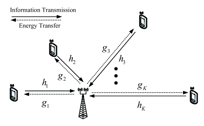
Figure 1: System Model: A Wireless Powered Communications Network

In this paper, we consider a WPCN with one HAP and $K$ users. The HAP is assumed to be equipped with two antennas. One is for the downlink wireless energy transfer. The other one is used to receive the uplink information transmission from the users. All the user terminals are assumed to be equipped with one single antenna each. As shown in Fig. 1, the channel power gain of the downlink channel from the HAP to user $i$ is denoted by $g_{i}$. The channel power gain of the uplink channel from user $i$ to the HAP is denoted by $h_{i}$. For the convenience of exposition, all the channels involved are assumed to be block-fading [22], i.e., the channels remain constant during each transmission block, but possibly change from one block to another. It is also assumed that all these channel power gains are perfectly known at the HAP.

The frame structure for energy harvesting and information transmission over one transmission block is shown in Fig. 2. In each block, the HAP keeps broadcasting wireless energy to all the users with a constant transmit power using one of its antenna. The transmit power of the HAP is denoted by $P_{H}$. To ensure tens of years of WPCN operations and small form factor for the users, the harvested energy is stored in supercapacitors. Since supercapacitors suffer from high self-discharge[15], we assume that the users can harvest energy before its transmission but not after. Hence, latter users can harvest more energy. We assume the users have no other energy source nor battery to store its harvested energy, and hence all harvested energy must be used for transmission with the frame. A TDMA structure is employed by the HAP to receive the uplink information transmission from the users. For convenience, we assume user $i$ transmits during the time slot $i$. The uplink transmission time for user $i$ is denoted by $\tau_{i}$, $\forall i\in\{1,\cdots,K\}$.

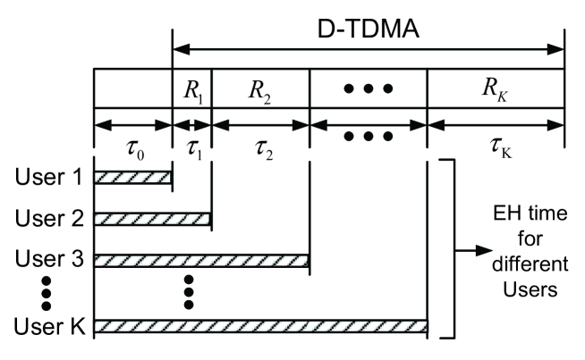
Figure 2: Frame structure for energy harvesting and information transmission. Latter users can harvest more energy.

Then, the energy harvesting time of user $i$ is given by $\sum_{j=0}^{i-1}\tau_{j},~{}\forall i\in\{1,2,\cdots,K\}$. Then, the total energy harvested by user $i$ from the HAP, denoted as $E_{i}$, can be obtained as

$$E_{i}=\eta_{i}\sum_{j=0}^{i-1}g_{i}P_{H}\tau_{j},~{}\forall i\in\{1,2,\cdots,K\},$$ (1)

where $\eta_{i}\in(0,1)$ is a constant denoting the energy harvesting efficiency for user $i$.

The average transmit power $p_{i}$ for user $i$ during its transmission slot is given by

$$p_{i}=\frac{E_{i}}{\tau_{i}},~{}\forall i\in\{1,2,\cdots,K\}.$$ (2)

Since TDMA is employed, each user can only transmit during its allocated time slot, and thus there is no mutual interference among the users. Besides, we assume that the HAP is equipped with a successive interference cancellation decoder. Thus, the interference from the downlink energy signal can be decoded first, and then be subtracted from the received signal. Then, the instantaneous uplink transmission rate for user $i$ can be written as

$$R_{i} =\ln\left(1+\frac{h_{i}E_{i}}{\tau_{i}\sigma^{2}}\right),$$

$$=\ln\left(1+\frac{\gamma_{i}\sum_{j=0}^{i-1}\tau_{j}}{\tau_{i}}\right),~{}\forall i\in\{1,2,\cdots,K\},$$ (3)

where $\gamma_{i}$ is defined as $\gamma_{i}=\frac{h_{i}\eta_{i}g_{i}P_{H}}{\sigma^{2}}$, $\forall i\in\{1,2,\cdots,K\}$, and $\sigma^{2}$ is the noise power at the HAP.

In this paper, we are interested in the following two problems: (i). Sum-throughput maximization, i.e., maximize the total throughput of the proposed WPCN subject to a total time constant $T$. (ii). Total-time minimization, i.e., minimize the total charging and transmission time of the proposed WPCN subject to the constraints that each user has certain amount of data to send back to the HAP. These two problems are investigated in the following two sections, respectively.

III Sum-throughput Maximization

III-A Problem Formulation

Define $\boldsymbol{\tau}=[\tau_{0},~{}\cdots,~{}\tau_{K}]^{T}$, the total throughput denoted by $\mathcal{T}(\boldsymbol{\tau})$ of the system is

$$\mathcal{T}(\boldsymbol{\tau}) =\sum_{i=1}^{K}\tau_{i}R_{i},$$

$$=\sum_{i=1}^{K}\tau_{i}\ln\left(1+\frac{\gamma_{i}\sum_{j=0}^{i-1}\tau_{j}}{\tau_{i}}\right),$$ (4)

where $\gamma_{i}$ is defined as $\gamma_{i}=\frac{h_{i}\eta_{i}g_{i}P_{H}}{\sigma^{2}}$, $\forall i\in\{1,2,\cdots,K\}$.

In this section, we are interested in finding the optimal time allocation strategy to maximize the total throughput $\mathcal{T}(\boldsymbol{\tau})$ of the described WPCN subject to a time constant $T$. For convenience, we use a normalized unit block time, i.e., $T=1$. Thus, the throughput maximization problem can be formulated as

Problem 1

$$\max_{\boldsymbol{\tau}} \sum_{i=1}^{K}\tau_{i}\ln\left(1+\frac{\gamma_{i}\sum_{j=0}^{i-1}\tau_{j}}{\tau_{i}}\right),$$ (5)

s.t. $$~{}\tau_{i}\geq 0,~{}\forall i\in\{0,1,2,\cdots,K\},$$ (6)

$$\sum_{i=0}^{K}\tau_{i}\leq 1.$$ (7)

Problem 1 is a convex optimization problem. To show this, we first present the following lemma.

Lemma 1

The throughput function of user $i$ given by $\mathcal{T}_{i}(\boldsymbol{\tau})\triangleq\tau_{i}\ln\left(1+\frac{\gamma_{i}\sum_{j=0}^{i-1}\tau_{j}}{\tau_{i}}\right)$, $\forall i\in\left\{1,\cdots,K\right\}$, is a concave function of $\boldsymbol{\tau}=[\tau_{0},~{}\cdots,~{}\tau_{K}]^{T}\succcurlyeq\boldsymbol{0}$.

Proof:

According to [23], a function is concave if its Hessian is negative semidefinite. Thus, to show $\mathcal{T}_{i}(\boldsymbol{\tau})$ is a concave function of $\boldsymbol{\tau}$, we have show that its Hessian is negative semidefinite. Denote the Hessian of $\mathcal{T}_{i}(\boldsymbol{\tau})$ by $\boldsymbol{H}_{i}$ and denote its element by $d_{m,n}^{(i)}$ at the $m$th row and $n$th column. The diagonal entries of $\boldsymbol{H}_{i}$, i.e., $m=n$, can be obtained as

$$d_{m,m}^{(i)}=\left\{\begin{array}[]{cc}-\frac{\gamma_{i}^{2}\tau_{i}}{\left(\gamma_{i}\sum_{j=0}^{i-1}\tau_{j}+\tau_{i}\right)^{2}},&~{}m<i,\\ -\frac{\gamma_{i}^{2}(\sum_{j=0}^{i-1}\tau_{j})^{2}}{\tau_{i}\left(\gamma_{i}\sum_{j=0}^{i-1}\tau_{j}+\tau_{i}\right)^{2}},&~{}m=i,\\ 0,&~{}m>i.\end{array}\right.$$ (11)

The off-diagonal entries of $\boldsymbol{H}_{i}$ can be obtained as

$$d_{m,n}^{(i)}=\left\{\begin{array}[]{cc}-\frac{\gamma_{i}^{2}\tau_{i}}{\left(\gamma_{i}\sum_{j=0}^{i-1}\tau_{j}+\tau_{i}\right)^{2}},&~{}m<i~{}\mbox{and}~{}n<i,\\ 0,&~{}m>i~{}\mbox{or}~{}n>i,\\ -\frac{\gamma_{i}^{2}\sum_{j=0}^{i-1}\tau_{j}}{\left(\gamma_{i}\sum_{j=0}^{i-1}\tau_{j}+\tau_{i}\right)^{2}},&~{}\mbox{otherwise}.\end{array}\right.$$ (15)

For any given real vector $\boldsymbol{v}=[v_{0},~{}\cdots,~{}v_{K}]^{T}$, it follows that

$$\boldsymbol{v}^{T}\boldsymbol{H}_{i}\boldsymbol{v} =-\frac{\gamma_{i}^{2}}{\tau_{i}\left(\gamma_{i}\sum_{j=0}^{i-1}\tau_{j}+\tau_{i}\right)^{2}}\left(\tau_{i}\sum_{j=0}^{i-1}v_{j}-v_{i}\sum_{j=0}^{i-1}\tau_{j}\right)^{2}$$

$${\leq}0,$$ (16)

where the inequality follows from the fact that $\tau_{i}\geq 0$. Thus, $\boldsymbol{H}_{i}$ is negative semidefinite. Lemma 1 is then proved. ∎

Proposition 1

Problem 1 is a convex optimization problem.

Proof:

According to [23], a nonnegative weighted summation of concave functions is concave. Then, it follows from Lemma 1 that the objective function of Problem 1 given by (1) is a concave function of $\boldsymbol{\tau}$ since it is a summation of $\mathcal{T}_{i}(\boldsymbol{\tau})$’s. Besides, all the constraints of Problem 1 are affine. Thus, it is clear that Problem 1 is a convex optimization problem. ∎

Another important feature of Problem 1 is presented in the following proposition.

Proposition 2

The optimal time allocation $\boldsymbol{\tau}^{*}=[\tau_{0}^{*},~{}\cdots,~{}\tau_{K}^{*}]^{T}$ of Problem 1 must satisfy $\sum_{i=0}^{K}\tau_{i}^{*}=1$.

Proof:

This can be proved by contradiction. Suppose $\boldsymbol{\tau}^{\prime}=[\tau_{0}^{\prime},~{}\cdots,~{}\tau_{K}^{\prime}]^{T}$ is an optimal solution of Problem 1, and it satisfies that $\sum_{i=0}^{K}\tau_{i}^{\prime}<1$. It follows that $\tau_{0}^{\prime}<1-\sum_{i=1}^{K}\tau_{i}^{\prime}$. It is easy to verify that the objective function given in (5) is a monotonic increasing function with respect to $\tau_{0}$. Thus, the value of (5) under the vector $[1-\sum_{i=1}^{K}\tau_{i}^{\prime},~{}\tau_{1}^{\prime},~{}\cdots,~{}\tau_{K}^{\prime}]^{T}$ is larger than that under $\boldsymbol{\tau}^{\prime}$. This contradicts with our presumption. Thus, the optimal $\boldsymbol{\tau}^{*}$ must satisfy $\sum_{i=0}^{K}\tau_{i}^{*}=1$. ∎

III-B Optimal Solution

In this subsection, we derive the optimal solution of Problem 1 using convex optimization techniques.

The Lagrangian of Problem 1 is

$$\mathcal{L}\left(\boldsymbol{\tau},\lambda\right)=\sum_{i=1}^{K}\tau_{i}\ln\left(1+\frac{\gamma_{i}\sum_{j=0}^{i-1}\tau_{j}}{\tau_{i}}\right)-\lambda\left(\sum_{i=0}^{K}\tau_{i}-1\right),$$ (17)

where $\lambda$ is the non-negative Lagrangian dual variable associated with the constraint given in (7).

Then, the dual function of Problem 1 can be written as

$$\mathcal{G}(\lambda)=\min_{\boldsymbol{\tau}\in\mathcal{S}}\mathcal{L}\left(\boldsymbol{\tau},\lambda\right),$$ (18)

where $\mathcal{S}$ is the feasible set of $\boldsymbol{\tau}$ specified by the constraints (6) and (7). It is observed that there exists an $\boldsymbol{\tau}\in\mathcal{S}$ with all strict positive element (i.e., $\tau_{i}>0,\forall i\in\{0,1,\cdots,K\}$) satisfying $\sum_{i=0}^{K}\tau_{i}<1$. Thus, according to the Slater’s condition [23], strong duality holds for this problem. Thus, Problem 1 can be solved by solving its Karush-Kuhn-Tucker (KKT) conditions, which are given by

$$\sum_{i=0}^{K}\tau^{*}_{i} \leq 1,$$ (19)

$$\lambda^{*}\left(\sum_{i=0}^{K}\tau^{*}_{i}-1\right) =0,$$ (20)

$$\frac{\partial\mathcal{L}\left(\boldsymbol{\tau},\lambda^{*}\right)}{\partial\tau_{i}}\Big{|}_{\tau_{i}=\tau_{i}^{*}} =0,~{}\forall i\in\{0,1,\cdots,K\},$$ (21)

where $\tau_{i}^{*},\forall i$ and $\lambda^{*}$ denote the optimal primal and dual solutions of Problem 1. Then, from (21), it follows that

$$\sum_{k=1}^{K}\frac{\gamma_{k}}{\gamma_{k}\frac{\sum_{j=0}^{k-1}\tau_{j}^{*}}{\tau_{k}^{*}}+1}=\lambda^{*}$$ , (22)

$$\mathcal{B}_{i}\left(\frac{\sum_{j=0}^{i-1}\tau_{j}^{*}}{\tau_{i}^{*}}\right)+\sum_{k=i+1}^{K}\frac{\gamma_{k}}{\gamma_{k}\frac{\sum_{j=0}^{k-1}\tau_{j}^{*}}{\tau_{k}^{*}}+1}=\lambda^{*}$$ ,

$$\forall i\in\{1,\cdots,K-1\}$$ . (23)

$$\mathcal{B}_{K}\left(\frac{\sum_{j=0}^{i-1}\tau_{j}^{*}}{\tau_{i}^{*}}\right)=\lambda^{*}$$ , (24)

where $\mathcal{B}_{i}(x)$ is defined as $\mathcal{B}_{i}(x)\triangleq\ln(1+\gamma_{i}x)-\frac{\gamma_{i}x}{1+\gamma_{i}x}$, $\forall i\in\{1,\cdots,K\}$.

It is observed that the right hand sides of equations (22)-(24) are the same. Thus, substituting (22) into (23) and (24), we have

$$\mathcal{B}_{1}\left(\frac{\tau_{0}^{*}}{\tau_{1}^{*}}\right)-\frac{\gamma_{1}}{\gamma_{1}\frac{\tau_{0}^{*}}{\tau_{1}^{*}}+1} =0,$$ (25)

$$~{}\vdots$$ (26)

$$\mathcal{B}_{K}\left(\frac{\sum_{j=0}^{K-1}\tau_{j}^{*}}{\tau_{K}^{*}}\right)-\kern-1.42262pt\frac{\gamma_{K}}{\gamma_{K}\frac{\sum_{j=0}^{K-1}\tau_{j}^{*}}{\tau_{K}^{*}}+1} =\sum_{k=1}^{K-1}\frac{\gamma_{k}}{\gamma_{k}\frac{\sum_{j=0}^{k-1}\tau_{j}^{*}}{\tau_{k}^{*}}+1}.$$ (27)

Now, we denote $\frac{\sum_{j=0}^{i-1}\tau_{j}^{*}}{\tau_{i}^{*}}$ by $x_{i}$, i.e.,

$$x_{i}\triangleq\frac{\sum_{j=0}^{i-1}\tau_{j}^{*}}{\tau_{i}^{*}},~{}\forall i\in\{1,\cdots,K\}.$$ (28)

We denote the right hand side of (25)-(27) by $c_{i}$, i.e.,

$$c_{1} \triangleq 0,$$ (29)

$$c_{i} \triangleq\sum_{k=1}^{i-1}\frac{\gamma_{k}}{\gamma_{k}x_{k}+1},\forall i\in\{2,\cdots,K\}.$$ (30)

For convenience, we introduce the following function

$$\mathcal{F}_{i}(x_{i})\triangleq\mathcal{B}_{i}(x_{i})-\frac{\gamma_{i}}{\gamma_{i}x_{i}+1},~{}\forall i\in\{1,\cdots,K\}.$$ (31)

Let $c_{i}\geq 0,\forall i\in\{1,\cdots,K\}$ be a series of constants, the solution of $\mathcal{F}_{i}(x)=c_{i}$ denoted by $x_{i}$ can be obtained as

$$x_{i}=\frac{1}{\gamma_{i}}\left(e^{\mathcal{W}\left(\frac{\gamma_{i}-1}{e^{c_{i}+1}}\right)+c_{i}+1}-1\right),\forall i\in\{1,\cdots,K\}.$$ (32)

where $\mathcal{W}\left(\cdot\right)$ is the Lambert W-Function [24].

It is observed from (32) that we need $c_{i}$ to compute $x_{i}$. When $i=1$, $x_{1}$ can be easily calculated since $c_{1}=0$. To compute $x_{2}$, we need the value of $c_{2}$. It is observed from (30) that $c_{2}$ can be easily computed if $x_{1}$ is known. Thus, $x_{2}$ can be computed with the obtained $x_{1}$. Similarly, for all other $i\geq 2$, it is observed from (30) that $c_{i}$ only depends on the value of previous $\{x_{1},\cdots,x_{i-1}\}$. Thus, using the same approach, all the remaining $x_{i}$ can be computed sequentially.

Now, we proceed to obtain the solution for $\tau_{i}^{*},\forall i\in\{1,\cdots,K\}$. Based on the fact that $\sum_{i=0}^{K}\tau^{*}_{i}=1$ and $\frac{\sum_{j=0}^{i-1}\tau_{j}^{*}}{\tau_{i}^{*}}=x_{i}$, $\forall i\in\{1,\cdots,K\}$, with the obtained value of $x_{i}$, the optimal $\tau_{i}^{*}$ can be obtained as

$$\tau_{K}^{*} =\frac{1}{1+x_{K}},$$ (33)

$$\tau_{i}^{*} =\frac{1-\sum_{j=i+1}^{K}\tau_{j}^{*}}{1+x_{i}},\forall i\in\{K-1,\cdots,1\},$$ (34)

$$\tau_{0}^{*} =1-(\tau_{K}^{*}+\cdots+\tau_{1}^{*}),$$ (35)

where $x_{i}$ is given by (32).

For convenience of computing the optimal time allocation, the following algorithm is proposed.

Algorithm 1 Optimal Time Allocation Computation

1:  Initialize: $c_{1}=0$, $x_{0}=0$,

2:  for i=1:K do

3:     $x_{i}=\frac{1}{\gamma_{i}}\left(e^{\mathcal{W}\left(\frac{\gamma_{i}-1}{e^{c_{i}+1}}\right)+c_{i}+1}-1\right)$,

4:     $c_{i+1}=\sum_{k=1}^{i}\frac{\gamma_{k}}{\gamma_{k}x_{k}+1}$,

5:  end for

6:  Compute $\tau_{K}$ by $\tau_{K}^{*}=\frac{1}{1+x_{K}}$.

7:  for i=K-1:0 do

8:     $\tau_{i}^{*}=\frac{1-\sum_{j=i+1}^{K}\tau_{j}^{*}}{1+x_{i}}$,

9:  end for

10:  Output: $\tau_{0}^{*},\cdots,\tau_{K}^{*}$.

It is observed that Algorithm 1 is a two-pass algorithm: One pass for sequentially computing $x_{i}$ and the other pass for computing $\tau_{i}$ in reverse order. Therefore, the algorithm need not be completely rerun when extending from $K$ users to $K+1$ users. Instead, we only need to rerun the second pass. This is due to the fact that the value $x_{K+1}$ does not affects the computation of $x_{i}$ with $i<K+1$, since the first pass is sequential. This indicates that the proposed algorithm has a good scalability.

Another interesting observation is that the sum throughput of the proposed WPCN is non-decreasing with the increasing of the number of users despite having the same total time constraint, which is given in the following theorem.

Theorem 1

The sum throughput of the proposed WPCN is non-decreasing with the increasing of the number of users.

Proof:

Consider there are $K$ users in the network. The optimal time allocation is $\boldsymbol{\tau}^{*}_{(K)}$ and the maximum throughput is $\mathcal{T}^{*}_{(K)}$. Now, we introduce one more user to the network, and recompute the optimal time allocation $\boldsymbol{\tau}^{\prime}_{(K+1)}$ and the maximum throughput $\mathcal{T}^{\prime}_{(K+1)}$. Now, we show that $\mathcal{T}^{\prime}_{(K+1)}\geq\mathcal{T}^{*}_{(K)}$.

This can be proved by contradiction. Suppose $\mathcal{T}^{\prime}_{(K+1)}<\mathcal{T}^{*}_{(K)}$. Now, we consider the following time allocation $\boldsymbol{\tau}^{\prime\prime}_{(K+1)}$ for the $K+1$ users case. We set the time allocation of the $K$ old users using $\boldsymbol{\tau}^{*}_{(K)}$ and set the time allocation of the new user using $0$. It is clear that under this time allocation, the resultant throughput denoted by $\mathcal{T}^{\prime\prime}_{(K+1)}$ is equal to $\mathcal{T}^{*}_{(K)}$. It follows that $\mathcal{T}^{\prime\prime}_{(K+1)}>\mathcal{T}^{\prime}_{(K+1)}$. This contradicts with our presumption. Thus, it follows $\mathcal{T}^{\prime}_{(K+1)}\geq\mathcal{T}^{*}_{(K)}$. ∎

IV Total-time Minimization

IV-A Problem Formulation

Let $D_{i}$ be the minimum amount of information that user $i$ has to send back to the HAP in each data collection cycle. Then, we have the following constraints

$$\tau_{i}\ln\left(1+\frac{\gamma_{i}\sum_{j=0}^{i-1}\tau_{j}}{\tau_{i}}\right)\geq D_{i},~{}\forall i\in\{1,2,\cdots,K\}.$$ (36)

We assume $D_{i}>0$ for all users, otherwise the user with $D_{i}=0$ can be omitted from the system to minimize the data collection time for that user.

In this section, we are interested in minimizing the completion time of charging and transmission of all users’ data in the proposed WPCN, i.e., $\sum_{i=1}^{K}\tau_{i}$, by determining the optimal time allocation strategy. Mathematically, this time minimization problem can be written as

Problem 2

$$\min_{\boldsymbol{\tau}}~{} \sum_{i=0}^{K}\tau_{i},$$ (37)

s. t. $$~{}\tau_{i}\geq 0,~{}\forall i\in\{0,1,2,\cdots,K\},$$ (38)

$$\tau_{i} \ln\left(1+\frac{\gamma_{i}\sum_{j=0}^{i-1}\tau_{j}}{\tau_{i}}\right)\geq D_{i},~{}\forall i\in\{1,2,\cdots,K\},$$ (39)

where $\boldsymbol{\tau}$ is defined as $\boldsymbol{\tau}=[\tau_{0},\cdots,\tau_{K}]^{T}$.

For convenience of expression, we refer to the constraint specified by (39) when $i=k$ as the $k$th constraint. First we observe that the $K$th constraint holds with equality.

Proposition 3

The optimal time allocation $\boldsymbol{\tau}^{*}$ of Problem 2 must satisfy the $K$th constraint with equality, i.e., $\tau_{K}^{*}\ln\left(1+\frac{\gamma_{K}\sum_{j=0}^{K-1}\tau_{j}^{*}}{\tau_{K}^{*}}\right)=D_{K}$.

Proof:

This can be proved by contradictory. Suppose an optimal solution $\tilde{\boldsymbol{\tau}}=[\tilde{\tau}_{0},\cdots,\tilde{\tau}_{K}]^{T}$ satisfying $\tau_{K}^{*}\ln\left(1+{\gamma_{K}\sum_{j=0}^{K-1}\tau_{j}^{*}}/{\tau_{K}^{*}}\right)>D_{K}$. Now, we consider the function $f(x)\triangleq x\log\left(1+c/x\right)$, where $c$ is a constant. It can be verified that $f(x)$ is a monotonic increasing function with respect to $x$ when $x>0$. Thus, by fixing $\tilde{\tau}_{0},\cdots,\tilde{\tau}_{K-1}$, we can always find a $\tau_{K}^{\prime}$ such that $\tau_{K}^{\prime}\ln\left(1+{\gamma_{K}\sum_{j=0}^{K-1}\tilde{\tau}_{j}}/{\tau_{K}^{\prime}}\right)=D_{K}$, and it is clear that $\tau_{K}^{\prime}<\tilde{\tau}_{K}$. This contradicts with our presumption that $\tilde{\boldsymbol{\tau}}$ is optimal. Thus, the optimal solution must satisfy the $K$th constraint with equality. ∎

We observe that each user’s energy harvesting time is coupled with the transmission time of all the users before him/her. It is the coupling among these constraints that makes the problem difficult to solve. Thus, to solve Problem 2, we first investigate the properties related that to the constraints. To this end, the constraints given in (39) can be rewritten as

$$\sum_{j=0}^{i-1}\tau_{j} \geq V_{i}(\tau_{i}),~{}\forall i\in\{1,2,\cdots,K\},$$ (40)

where $V_{i}(\tau_{i})$ is defined as

$$V_{i}(\tau_{i})\triangleq\frac{\tau_{i}}{\gamma_{i}}\left(e^{\frac{D_{i}}{\tau_{i}}}-1\right),~{}\forall i\in\{1,2,\cdots,K\}.$$ (41)

Proposition states that $V_{i}(\cdot)$ is a strictly decreasing function.

Proposition 4

The function $V_{i}(\tau_{i})$ is a strictly decreasing function with respect to $\tau_{i}$.

Proof:

First we note that $\tau_{i}>0$ so as to serve the strictly positive $D_{i}$. The first order derivative of $V_{i}(\tau_{i})$ is

$$\frac{dV_{i}(\tau_{i})}{d\tau_{i}} =-\frac{(D_{i}-\tau_{i})e^{D_{i}/\tau_{i}}+\tau_{i}}{\gamma_{i}\tau_{i}}$$

$$\stackrel{{\scriptstyle a}}{{<}}-\frac{(D_{i}-\tau_{i})+\tau_{i}}{\gamma_{i}\tau_{i}}<0$$ (42)

where the inequality “a” follows from $e^{x}>1$ for $x>0$ and the assumption that $D_{i}>0$. ∎

By using a graphical approach, the subsequent key result can be proved easily and key insights can be drawn intuitively. Hence, we illustrate the graphical relationship between the curve $V_{i}(\tau_{i})=\frac{\tau_{i}}{\gamma_{i}}\left(e^{\frac{D_{i}}{\tau_{i}}}-1\right)$ and the line $\sum_{j=0}^{i-1}\tau_{j}=-\tau_{i}+C_{i}$ in Fig. 3. We note that $C_{i}=\sum_{j=0}^{i}\tau_{j}$ represents the completion time until user $i$ sends its data; in particular $C_{K}$ is the total completion time that we want to minimize. Lemma 2 states the critical values of $C_{i}$ and $\tau_{i}$ when the curve and line meet at one unique point.

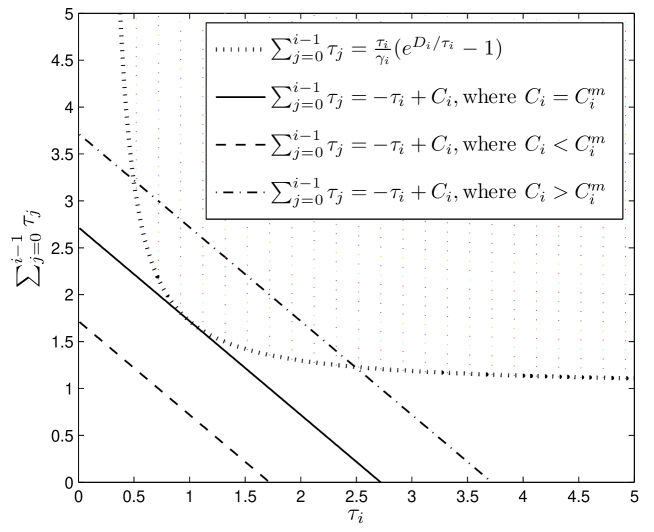
Figure 3: Graphic representation of the $i$th constraint

Lemma 2

Denote $C_{i}^{m}$ as $C_{i}$ such that the line $\sum_{j=0}^{i-1}\tau_{j}=-\tau_{i}+C_{i}$ has only one intersection point with the curve $V_{i}(\tau_{i})$. Denote the corresponding $\tau_{i}$ as $\tau_{i}^{m}$. Then

$$\tau_{i}^{m} =\frac{D_{i}}{\mathcal{W}\left(\frac{\gamma_{i}-1}{e}\right)+1}$$ (43)

$$C_{i}^{m} =\frac{D_{i}}{\gamma_{i}}e^{\mathcal{W}\left(\frac{\gamma_{i}-1}{e}\right)+1}.$$ (44)

where $\mathcal{W}\left(\cdot\right)$ is the Lambert W-Function [22].

Proof:

At the unique intersection point, we have

$$\left.\frac{dV_{i}(\tau_{i})}{d\tau_{i}}\right|_{\tau_{i}=\tau_{i}^{m}} =-1,$$ (45)

$$V_{i}(\tau_{i}^{m}) =-\tau_{i}^{m}+C_{i}^{m}.$$ (46)

From (45), it follows that $-\frac{(D_{i}-\tau_{i}^{m})e^{D_{i}/\tau_{i}^{m}}+\tau_{i}^{m}}{\gamma_{i}\tau_{i}^{m}}=-1$. Then, $\tau_{i}^{m}$ can be obtained as given in (43). From (46), it follows that $C_{i}^{m}=\frac{D_{i}}{\gamma_{i}}e^{\frac{D_{i}}{\tau_{i}^{m}}}$. Then, substituting (43) into this equation, $C_{i}^{m}$ can be obtained as given in (44). ∎

From Fig. 3, we have the following observations:

• When $C_{i}<C_{i}^{m}$, there is no intersection between the line and the curve. When $C_{i}>C_{i}^{m}$, there are two intersection points between the line and the curve.

• The shaded area is the feasible region specified by the $i$th constraint.

With these obtained properties and observations, we are now ready for solving Problem 2 optimally, which is presented in the following section.

IV-B Optimal Solution

In this subsection, we derive the optimal solution of Problem 2 based on the results obtained in the previous subsection.

Theorem 2

The optimal solution of Problem 2 is obtained at the largest $k$ such that: when $C_{k}=C_{k}^{m}$ and $\tau_{k}=\tau_{k}^{m}$, there exists a time allocation $[\tau_{0},\cdots,\tau_{k-1}]^{T}$ that satisfies the $(k-j)$th constraints, $\forall j=1,\cdots,k$.

Proof:

From the previous section, it is known that minimizing $\sum_{i=0}^{K}\tau_{i}$ is equivalent to minimizing $C_{K}$. Then, we plot the line $\sum_{i=0}^{K-1}\tau_{i}=-\tau_{K}+C_{K}$ and the curve $\sum_{i=0}^{K-1}\tau_{i}=\frac{\tau_{K}}{\gamma_{K}}\left(e^{\frac{D_{K}}{\tau_{K}}}-1\right)$ in Fig. 4(a). Since the curve represents the $K$th constraint, the minimum feasible $C_{K}$ under the $K$th constraint is $C_{K}=C_{K}^{m}$, and the corresponding $\tau_{K}$ is given by $\tau_{K}=\tau_{K}^{m}$, where $\tau_{K}^{m}$ and $C_{K}^{m}$ are computed by (43) and (44), respectively. Then, $C_{K-1}$ can be computed by $C_{K-1}=C_{K}-\tau_{K}=C_{K}^{m}-\tau_{K}^{m}$. Now, we have the following two possible cases:

• Case 1: $C_{K-1}>C_{K-1}^{m}$. From Fig. 4(b), it is observed that when $C_{K-1}>C_{K-1}^{m}$, there are two intersection points between the line $\sum_{i=0}^{K-2}\tau_{i}=-\tau_{K-1}+C_{K-1}$ and the curve $\sum_{i=0}^{K-2}\tau_{i}=\frac{\tau_{K-1}}{\gamma_{K-1}}\left(\exp(D_{K-1}/\tau_{K-1})-1\right)$. Denote the $\tau^{\prime}$ and $\tau^{\prime\prime}$, where $\tau^{\prime}<\tau^{\prime\prime}$, as the two solutions for $\tau$, see Fig. 4(b). In this case, we can choose any $\tau_{K-1}$ between $\tau^{\prime}$ and $\tau^{\prime\prime}$, and yet satisfy the $(K-1)$th constraint. However, from the perspective of satisfying the remaining constraints, we should choose the smallest possible $\tau_{K-1}$, i.e, choose $\tau_{K-1}=\tau^{\prime}$, due to the following. A smaller $\tau_{K-1}$ results in a larger $\sum_{i=0}^{K-2}\tau_{i}$, since from Proposition 4, $\sum_{i=0}^{K-2}\tau_{i}=\frac{\tau_{K-1}}{\gamma_{K-1}}\left(\exp(D_{K-1}/\tau_{K-1})-1\right)$ is a decreasing function with respective to $\tau_{K-1}$. Since $C_{K-2}=\sum_{i=0}^{K-2}\tau_{i}$, a larger $\sum_{i=0}^{K-2}\tau_{i}$ implies a larger $C_{K-2}$. A larger $C_{K-2}$ results in the most relaxed $(K-2)$th constraint, i.e., the largest possible feasible region. By induction, this also resulted in the most relaxed $(K-j)$th constraint for $j=3,\cdots,K-1$.

• Case 2: $C_{K-1}<C_{K-1}^{m}$. From Fig. 4(b), it is observed that when $C_{K-1}<C_{K-1}^{m}$, there is no intersection between the line $\sum_{i=0}^{K-2}\tau_{i}=-\tau_{K-1}+C_{K-1}$ and the curve $\sum_{i=0}^{K-2}\tau_{i}=\frac{\tau_{K-1}}{\gamma_{K-1}}\left(\exp(D_{K-1}/\tau_{K-1})-1\right)$, which means that the $(K-1)$th constraint is not satisfied. In order to satisfy the $(K-1)$th constraint, we must increase the value of $C_{K-1}$ to $C_{K-1}^{m}$. Since $C_{K-1}=C_{K}-\tau_{K}$, the value of $C_{K-1}$ can be increased by increasing $C_{K}$ or decreasing $\tau_{K}$. If we keep $C_{K}=C_{K}^{m}$ and only decrease the value of $\tau_{K}$, the $K$th constraint will not be satisfied. Thus, the value of $C_{K}$ must be increased. This indicates $C_{K}^{m}$ is no longer a feasible solution of Problem 2. Hence it is necessary to set the tentative optimal solution at $C_{K-1}=C_{K-1}^{m}$ and $\tau_{K-1}=\tau_{K-1}^{m}$.

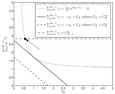
(a) The $K$th constraint

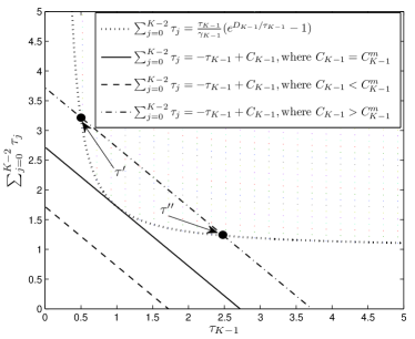
(b) The $(K\kern-2.84526pt-\kern-1.42262pt1\kern-1.13809pt)$th constraint

Figure 4: Graphic representation of the $K$th and $(K\kern-2.84526pt-\kern-1.42262pt1\kern-1.13809pt)$th constraints

If case 1 happens, and all the remaining $C_{K-j}$’s computed by the approach specified in case 1 satisfy $C_{K-j}>C_{K-j}^{m}$, $\forall j=2,\cdots,K-1$, the optimal solution is obtained at $C_{K}=C_{K}^{m}$ and $\tau_{K}=\tau_{K}^{m}$. If case 2 happens, we start from $C_{K-1}=C_{K-1}^{m}$ and $\tau_{K-1}=\tau_{K-1}^{m}$, and recomputed $C_{K-j}$, $\forall j=2,\cdots,K-1$. If all the computed $C_{K-j}$’s satisfy $C_{K-j}>C_{K-j}^{m}$, the optimal solution is now obtained at $C_{K-1}=C_{K-1}^{m}$ and $\tau_{K-1}=\tau_{K-1}^{m}$. Otherwise, we have to repeat this procedure until we find the largest $k$ such that: when $C_{k}=C_{k}^{m}$ and $\tau_{k}=\tau_{k}^{m}$, all the computed $C_{k-j}$’s satisfy $C_{k-j}\geq C_{k-j}^{m},~{}\forall j=1,\cdots,k-1$.

Theorem 2 is thus proved. ∎

Thus, the optimal solution of Problem 2 can be obtained in the following two steps: (i) Find the largest $k$ specified in Theorem 2. (ii) Let $C_{k}=C_{k}^{m}$ and $\tau_{k}=\tau_{k}^{m}$, and then solve for the remaining the $C_{i}$’s and $\tau_{i}$’s.

The pseudocode for finding the largest $k$ specified in Theorem 2 is given in Algorithm 2. In Line 8 of Algorithm 2, the operator Root finds the smaller of the two roots in the equation, i.e., $\tau_{i}^{\prime}$ in Fig. 4(b).

Algorithm 2 Finding the largest $k$ specified in Theorem 2

1:  Initialize: $\mbox{Flag}=0$, $k=0$.

2:  Compute $\tau_{i}^{m}=\frac{D_{i}}{\mathcal{W}\left(\frac{\gamma_{i}-1}{e}\right)+1}$, $C_{i}^{m}=\frac{D_{i}}{\gamma_{i}}e^{\mathcal{W}\left(\frac{\gamma_{i}-1}{e}\right)+1}$, $\forall i=1,\cdots,K$.

3:  for $j=K:-1:1$ do

4:     if $j>1$ then

5:        $C_{j-1}=C_{j}^{m}-\tau_{j}^{m}$;

6:        for $i=j-1:-1:1$ do

7:           if $C_{i}\geq C_{i}^{m}$ then

8:              $\tau_{i}=\min\left\{\mbox{Root}\left(\frac{\tau_{i}}{\gamma_{i}}\left(e^{\frac{D_{i}}{\tau_{i}}}-1\right)=-\tau_{i}+C_{i}\right)\right\}$;

9:              if $i>1$ then

10:                 $C_{i-1}=C_{i}-\tau_{i}$;

11:              else

12:                 $\mbox{Flag}=1$;

13:              end if

14:           else

15:              $j=i$;

16:              break;

17:           end if

18:        end for

19:     end if

20:     if $\mbox{Flag}==1$ then

21:        Output: $k=j$.

22:        break;

23:     end if

24:     Output: $k=1$.

25:  end for

Using Algorithm 2, we can easily find the largest $k$ specified by Theorem 2. Then, it follows that $C_{k}^{*}=C_{k}^{m}$ and $\tau_{k}^{*}=\tau_{k}^{m}$. With this result, for any $i<k$, $C_{i}$’s and $\tau_{i}$’s can be easily obtained by using the same method as Algorithm 2 (line $4$ to line $10$). Now, we show how to compute $C_{i}$’s and $\tau_{i}$’s for any $i>k$. In this case, $C_{K}$ can be obtained by $C_{i+1}^{*}=C_{i}^{*}+\tau_{i+1}^{*}$, where $\tau_{i+1}^{*}$ is obtained by solving the equation $\frac{\tau_{i+1}^{*}}{\gamma_{i+1}}\left(e^{\frac{D_{i+1}}{\tau_{i+1}^{*}}}-1\right)=C_{i}^{*}$. The solution of this equation is unique since the curve $\sum_{i=0}^{i}\tau_{i}=\frac{\tau_{i+1}}{\gamma_{i+1}}\left(e^{\frac{D_{i+1}}{\tau_{i+1}}}-1\right)$ is a monotonic decreasing function of $\tau_{i+1}$, and $\sum_{i=0}^{i}\tau_{i}=C_{i}$ is a horizontal line, which is illustrated in Fig. 4(a). The approach to compute the optimal time allocation presented above is summarized in the following algorithm.

Algorithm 3 Optimal time allocation computation

1:  Input: $k$, which is obtained by Algorithm 2.

2:  Initialize: $C_{k}^{*}=C_{k}^{m}$ and $\tau_{k}^{*}=\tau_{k}^{m}$.

3:  Compute $C_{k-1}^{*}=C_{k}^{*}-\tau_{k}^{*}$.

4:  for $i=k-1:-1:1$ do

5:     $\tau_{i}^{*}=\min\left\{\mbox{Root}\left(\frac{\tau_{i}^{*}}{\gamma_{i}}\left(e^{\frac{D_{i}}{\tau_{i}^{*}}}-1\right)=-\tau_{i}^{*}+C_{i}^{*}\right)\right\}$;

6:     $C_{i-1}^{*}=C_{i}^{*}-\tau_{i}^{*}$.

7:  end for

8:  for $i=k+1:+1:K$ do

9:     $\tau_{i}^{*}=\mbox{Root}\left(\frac{\tau_{i}^{*}}{\gamma_{i}}\left(e^{\frac{D_{i}}{\tau_{i}^{*}}}-1\right)=C_{i-1}^{*}\right)$;

10:     $C_{i}^{*}=C_{i-1}^{*}+\tau_{i}^{*}$.

11:  end for

12:  $\tau_{0}^{*}=C_{1}^{*}-\tau_{1}^{*}$.

13:  Output: $\tau_{0}^{*},\cdots,\tau_{K}^{*}$.

Algorithm 3 is an efficient way to obtain an optimal solution of Problem 2. However, it is worth pointing out that:

• The optimal time allocation of Problem 2 may not be unique when $K\geq 2$. We use a simple example to illustrate this. Consider the case that $K=2$. We assume that $C_{1}=C_{2}-\tau_{2}>C_{1}^{m}$, when $C_{2}=C_{2}^{m}$ and $\tau_{2}=\tau_{2}^{m}$. Then, any time allocation on the line $\tau_{0}=-\tau_{1}+C_{1}$ within the feasible region $\tau_{0}\geq\frac{\tau_{1}}{\gamma_{1}}\left(e^{\frac{D_{1}}{\tau_{1}}}-1\right)$ are optimal time allocation.

• When $K=1$, the optimal time allocation of Problem 2 is unique, and is given by $\tau_{1}=^{*}\frac{D_{1}}{\mathcal{W}\left(\frac{\gamma_{1}-1}{e}\right)+1}$ and $\tau_{0}^{*}=\frac{\tau_{1}^{*}}{\gamma_{1}}\left(e^{\frac{D_{1}}{\tau_{1}^{*}}}-1\right)$. Details are omitted for brevity.

V Suboptimal Time Allocation

In this section, we propose some suboptimal time allocation schemes for the sum-throughput maximization and the total-time minimization problems, respectively. The motivation for proposing these suboptimal time allocation schemes is two-folds: (i). To see whether optimization helps in improving the system performance. (ii). To develop the low-complexity schemes that can achieve near-optimal performance.

V-A Sum-throughput maximization

In this subsection, we propose two suboptimal time allocation schemes for the sum-throughput maximization problem, which are given as follows.

(i). Equal time allocation. The idea of this scheme is to allocate equal time to each user including the initial charging slot $\tau_{0}$, i.e., $\tau_{i}=\tau_{0}$, $\forall i\in\{1,\cdots,K\}$. Then, since $\sum_{i=0}^{K}\tau_{i}=1$, it follows that

$$\tau_{i}=\frac{1}{K+1},\forall i\in\{0,1,\cdots,K\}.$$ (47)

(ii). Fixed-TDMA allocation: The idea of this scheme is to allocate equal time to each user but leave the initial charing slot $\tau_{0}$ as an optimization variable. Thus, it follows that

$$\tau_{i}=\frac{1-\tau_{0}}{K},\forall i\in\{1,\cdots,K\}.$$ (48)

Substituting the above equation into Problem 1, it follows that

Problem 3

$$\max_{\tau_{0}} \sum_{i=1}^{K}\frac{1-\tau_{0}}{K}\ln\left(i+\frac{K\gamma_{i}\tau_{0}}{1-\tau_{0}}\right),$$ (49)

s.t. $$~{}0\leq\tau_{0}\leq 1,$$ (50)

Now, we show that Problem 1 is a convex optimization problem. To show this, we present the following lemma first.

Lemma 3

The function of user $i$ given by $\mathcal{T}^{\prime}_{i}(\tau_{0})\triangleq\frac{1-\tau_{0}}{K}\ln\left(i+\frac{K\gamma_{i}\tau_{0}}{1-\tau_{0}}\right)$, $\forall i\in\left\{1,\cdots,K\right\}$ is a concave function of $\tau_{0}$ when $0\leq\tau_{0}\leq 1$.

Proof:

This can be proved by looking at the second order derivative of $\mathcal{T}^{\prime}_{i}(\tau_{0})$, which is

$$\frac{d^{2}\mathcal{T}^{\prime}_{i}(\tau_{0})}{dx^{2}} =\frac{\gamma_{i}^{2}K}{(\tau_{0}-1)(\tau_{0}(\gamma_{i}K-i)+i)^{2}}$$

$$\stackrel{{\scriptstyle a}}{{\leq}}0,$$ (51)

where “a” follows from the fact that $0\leq\tau_{0}\leq 1$. Thus, it is clear that $\mathcal{T}^{\prime}_{i}(\tau_{0})$ is concave function of $\tau_{0}$ when $0\leq\tau_{0}\leq 1$. ∎

Based on Lemma 3, it is easy to observe that the objective function of Problem 3 is a concave function of $\tau_{0}$ when $0\leq\tau_{0}\leq 1$, since the summation operation preserves the concavity [23]. Since Problem 3 is a convex optimization problem with one optimization variable, it can be easily solved by the subgradient method [25]. Details are omitted here for brevity.

V-B Total-time minimization

In this subsection, we propose two suboptimal time allocation schemes for the total-time minimization problem, which are given as follows.

(i). Equal time allocation. The idea of this scheme is to allocate equal time to each user including the initial charging slot $\tau_{0}$, i.e., $\tau_{i}=\tau_{0}$, $\forall i\in\{1,\cdots,K\}$. Substituting this condition into Problem (2), the problem is simplified as

Problem 4

$$\min_{\boldsymbol{\tau}}~{} \tau_{0},$$ (52)

s. t. $$~{}\tau_{0}\ln\left(1+i\gamma_{i}\right)\geq D_{i},\forall i\in\{1,\cdots,K\}.$$ (53)

The optimal solution for this problem can be easily obtained, which is

$$\tau_{0}=\mbox{argmax}_{i}\frac{D_{i}}{\ln\left(1+i\gamma_{i}\right)}.$$ (54)

(ii). Tangent-point allocation: This scheme is inspired by the graphic method used for deriving the optimal solution of Problem 2. The idea of this scheme is to let $\tau_{i}$ takes the value of the tangent-point illustrated in Fig. 3 for all $i$, i.e.,

$$\widetilde{\tau}_{i} =\frac{D_{i}}{\mathcal{W}\left(\frac{\gamma_{i}-1}{e}\right)+1},\forall i=1,\cdots,K,$$ (55)

and $\widetilde{\tau}_{0}$ is given by the smallest value such that all the constraints given in (39) are satisfied. Since the left hand side of each constraint given in (39) is a monotonic increasing function with respect to $\tau_{0}$. Thus, $\tau_{0}$ can be easily found by the well-known bisection search [23]. Details are omitted here for brevity.

VI Numerical Results

In this section, several numerical examples are presented to evaluate the performance of the proposed algorithms.

VI-A Simulation setup

In the simulation, the power of the noise $\sigma^{2}$ at the receiver of the HAP is assumed to be one. For simplicity, the energy harvest efficiency for all users are assumed to be the same and equal to one, i.e., $\eta_{i}=1,\forall i$. The amount of data that each user has to send back is assumed to be the same and equal to one, i.e., $D_{i}=1,\forall i$. We assume i.i.d. Rayleigh fading for all channels involved, and thus the channel power gains of these channels are exponentially distributed. For convenience, we assume that the mean of the channel power gains is one. It is worth pointing out that the assumption of particular distributions of the channel power gains does not affect the structure of the problem studied and the algorithm proposed in this paper. The results given in the following examples are obtained by averaging over $1000$ channel realizations.

Figure 5: Throughput vs. HAP’s transmit power ($P_{H}$)

VI-B Sum-throughput maximization

VI-B1 Effect of the user scheduling

In Fig. 5, we investigate the effect of user scheduling on the throughput of the proposed system. We consider two scheduling schemes: (i) Increasing order of SNRs, i.e., the user with lowest SNR is scheduled to transmit first; (ii) Decreasing order of SNRs, i.e., the user with highest SNR is scheduled to transmit first. For exposure, we assume that there are five users in the network, i.e., $K=5$. It is observed from Fig. 5 that the increasing order scheduling scheme performs better than the decreasing order scheduling scheme. It is also observed that the throughput gap between the two scheduling schemes increases with the increasing of $P_{H}$. This indicates that user scheduling is more important when $P_{H}$ is large.

VI-B2 Optimal Vs. Suboptimal Time Allocation

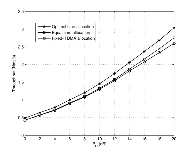
Figure 6: Throughput vs. HAP’s transmit power ($P_{H}$)

In Fig. 6, we investigate the effect of the transmit power of the HAP on the throughput of the proposed system under the optimal time allocation and that under the equal time allocation. In this example, for simplicity, we consider the case that there are two users, i.e., $K=2$. It is observed that the optimal time allocation always perform better than the suboptimal time allocation. It is also observed from Fig. 6 that the throughput for all cases increases when the transmit power of the HAP ($P_{H}$) increases as expected. A higher $P_{H}$ indicates that the users can harvest more energy from the HAP, and thus can transmit at higher transmission rates. Therefore, the throughput of the system increases. Another important observation is that the throughput gap between the optimal time allocation and the equal time allocation increases with the increasing of $P_{H}$. This indicates that time allocation plays a more important role when $P_{H}$ is large.

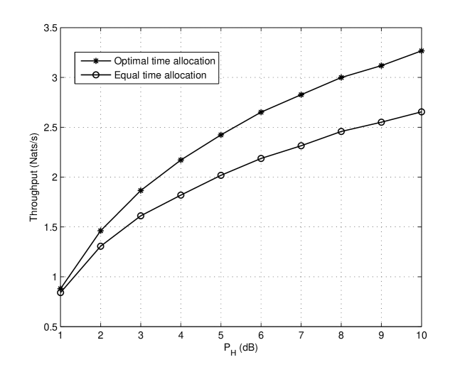
Figure 7: Throughput vs. Number of users ($K$)

In Fig. 7, we investigate the effect of the number of users on the throughput of the proposed system under the optimal time allocation and that under the equal time allocation. In this example, the transmit power of the HAP is fixed at $P_{H}=10~{}dB$. It is observed that the throughput gap between the optimal time allocation and the equal time allocation increases with the increasing of the number of users ($K$). It is observed from Fig. 7 that when $K=1$, the gap is negligible. However, when $K=10$, the gap is as large as $1$. This indicates that time allocation plays a more important role when $K$ is large. Another important observation is that the throughput for both cases increases when the number of users increases. This is in accordance to the results presented in Theorem 1.

VI-C Total-time minimization

VI-C1 Effect of the user scheduling

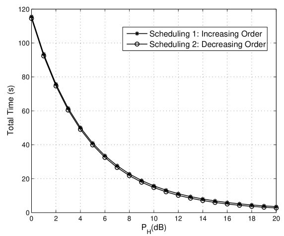
Figure 8: Total time vs. HAP’s transmit power ($P_{H}$)

In Fig. 8, we investigate the effect of the user scheduling on the total data collection time of the proposed WPCN. We consider two scheduling schemes: (i) Increasing order of SNRs, i.e., the user with lowest SNR is scheduled to transmit first; (ii) Decreasing order of SNRs, i.e., the user with highest SNR is scheduled to transmit first. For exposure, we assume that there are five users in the network, i.e., $K=5$. It is observed from Fig. 8 that the increasing order scheduling scheme performs worse than the decreasing order scheduling scheme, the gap between the two scheduling schemes is, however, quite small. One of the possible reasons is that users with good SNRs finish their data transmission very fast, and thus contributes a negligible part of the total time. On the other hand, users with the poor SNRs require long charging and transmission time. Thus, the users with poor SNRs determine the overall performance. Another observation is that the total time decreases with the increasing of $P_{H}$. This is as expected, since higher $P_{H}$ indicates that the users can harvest more energy from the HAP, and thus can transmit at higher transmission rates.

VI-C2 Optimal Vs. Suboptimal Time Allocation

In this subsection, we compare the performance of suboptimal time allocation with the optimal time allocation.

In Fig. 6, we compare the performance of the proposed suboptimal time allocation with that of the optimal time allocation.For exposure, we assume that there are five users in the network, i.e., $K=5$. The equal time allocation is not included here due to its poor performance. This also indicates that optimization is necessary and helps in improving the system performance. As expected, it is observed that the optimal time allocation always perform better than tangent point allocation. It is also observed that the gap between the optimal and the tangent point allocation is very small. This indicates that the tangent point allocation scheme has a very good performance. Another observation is that the total time decreases with the increasing of $P_{H}$, and the gap also decreases with the increasing of $P_{H}$.

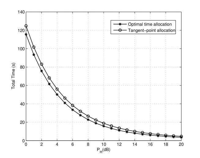
Figure 9: Optimal vs. Suboptimal time allocation

VII Conclusions

In this paper, we have proposed a new protocol to enable simultaneous downlink wireless power transfer (WPT) and uplink information transmission for a wireless communication network with a full-duplex hybrid access point (HAP) and a set of wireless users with energy harvesting capabilities. Time-division-multiple-access (TDMA) is employed to realize the multi-user uplink transmission. All users can continuously harvest wireless power from the HAP until its transmission slot, even during other users’ uplink transmission. Consequently, latter users’ energy harvesting time is coupled with the transmission time of previous users. Under this setup, we have investigated the sum-throughput maximization (STM) problem and the total-time minimization (TTM) problem for the proposed multi-user full-duplex wireless-powered network, respectively. We have proved that the STM problem is a convex optimization problem. The optimal solution strategy has been obtained in closed-form expression. An algorithm with linear complexity is then given for the convenience of computation. We have shown that the sum-throughput is non-decreasing with the increasing of the number of users. For the TTM problem, we have proposed a two-step algorithm to obtain an optimal solution by exploring the properties of the coupling constraints. Then, we have proposed several suboptimal solutions are each problem. We also have investigated the effect of user scheduling on STM and TTM through simulations. We have shown that different user scheduling strategies should be used for STM and TTM.

References

- [1] O. Ozel, K. Tutuncuoglu, J. Yang, S. Ulukus, and A. Yener, “Transmission with energy harvesting nodes in fading wireless channels: Optimal policies,” IEEE J. Sel. Areas Commun., vol. 29, no. 8, pp. 1732–1743, Sept. 2011.
- [2] C. K. Ho and R. Zhang, “Optimal energy allocation for wireless communications with energy harvesting constraints,” IEEE Trans. Signal Process., vol. 60, no. 9, pp. 4808–4818, Sept. 2012.
- [3] L. R. Varshney, “Transporting information and energy simultaneously,” in Proc. IEEE ISIT, 2008, pp. 1612–1616.
- [4] N. Shinohara, “Power without wires,” IEEE Microwave Magazine, vol. 12, no. 7, pp. S64–S73, Dec 2011.
- [5] V. Liu, A. Parks, V. Talla, S. Gollakota, D. Wetherall, and J. R. Smith, “Ambient backscatter: wireless communication out of thin air,” in Proc. ACM SIGCOMM, 2013, pp. 39–50.
- [6] K. Finkenzeller, “RFID handbook: Fundamentals and applications in contactless smart cards and identification,” 2003.
- [7] J. R. Smith, Wirelessly Powered Sensor Networks and Computational RFID. Springer, 2013.
- [8] P. Grover and A. Sahai, “Shannon meets tesla: wireless information and power transfer,” in Proc. IEEE ISIT, 2010, pp. 2363–2367.
- [9] R. Zhang and C. K. Ho, “MIMO broadcasting for simultaneous wireless information and power transfer,” IEEE Trans. Wireless Commun., vol. 12, no. 5, pp. 1989–2001, May 2013.
- [10] L. Liu, R. Zhang, and K. C. Chua, “Wireless information and power transfer: a dynamic power splitting approach,” IEEE Trans. Commun., vol. 61, no. 9, pp. 3990–4001, Sept. 2013.
- [11] X. Zhou, R. Zhang, and C. K. Ho, “Wireless information and power transfer: architecture design and rate-energy tradeoff,” IEEE Trans. Commun., vol. 61, no. 11, pp. 4757–4767, Nov. 2013.
- [12] K. Huang and V. K. N. Lau, “Enabling wireless power transfer in cellular networks: architecture, modeling and deployment,” IEEE Trans. Wireless Commun., vol. PP, no. 99, pp. 1–11, Jan. 2014.
- [13] G. Yang, C. K. Ho, and Y. L. Guan, “Dynamic resource allocation for multiple-antenna wireless power transfer,” arXiv:1311.4111, 2013.
- [14] F. Simjee and P. H. Chou, “Everlast: long-life, supercapacitor-operated wireless sensor node,” in Proceedings of the 2006 International Symposium on Low Power Electronics and Design. IEEE, 2006, pp. 197–202.
- [15] M. Kaus, J. Kowal, and D. U. Sauer, “Modelling the effects of charge redistribution during self-discharge of supercapacitors,” Electrochimica Acta, vol. 55, no. 25, pp. 7516–7523, 2010.
- [16] D. Bharadia, E. McMilin, and S. Katti, “Full duplex radios,” in Proc. ACM SIGCOMM 2013, pp. 375–386.
- [17] H. Ju and R. Zhang, “Throughput maximization in wireless powered communication networks,” IEEE Trans. Wireless Commun., vol. 13, no. 1, pp. 418–428, Jan. 2014.
- [18] A. M. Fouladgar and O. Simeone, “On the transfer of information and energy in multi-user systems,” IEEE Commun. Lett., vol. 16, no. 11, pp. 1733–1736, Nov. 2012.
- [19] D. W. K. Ng, E. S. Lo, and R. Schober, “Energy-efficient resource allocation in multiuser ofdm systems with wireless information and power transfer,” in IEEE WCNC 2013, pp. 3823–3828.
- [20] A. A. Nasir, X. Zhou, S. Durrani, and R. A. Kennedy, “Relaying protocols for wireless energy harvesting and information processing,” IEEE Trans. Wireless Commun., vol. 12, no. 7, pp. 3622–3636, Jul. 2013.
- [21] K. Huang and E. Larsson, “Simultaneous information and power transfer for broadband wireless systems,” IEEE Trans. Signal Process., vol. 61, no. 23, pp. 5972–5986, Dec 2013.
- [22] X. Kang, Y.-C. Liang, A. Nallanathan, H. K. Garg, and R. Zhang, “Optimal power allocation for fading channels in cognitive radio networks: Ergodic capacity and outage capacity,” IEEE Trans. Wireless Commun., vol. 8, no. 2, pp. 940–950, 2009.
- [23] S. Boyd and L. Vandenberghe, Convex Optimization. Cambridge, UK: Cambridge University Press, 2004.
- [24] “Lambert W-function.” [Online]. Available: http://mathworld.wolfram.com/LambertW-Function.html
- [25] S. Boyd, L. Xiao, and A. Mutapcic, “Subgradient methods,” Lecture notes of EE392o, Stanford University, 2003.