Low-energy effective theories of the two-thirds filled Hubbard model on the triangular necklace lattice

Abstract

Motivated by Mo₃S₇(dmit)₃, we investigate the Hubbard model on the triangular necklace lattice at two-thirds filling. We show, using second order perturbation theory, that in the molecular limit, the ground state and the low energy excitations of this model are identical to those of the spin-one Heisenberg chain. The latter model is known to be in the symmetry protected topological Haldane phase. Away from this limit we show, on the basis of symmetry arguments and density matrix renormalization group (DMRG) calculations, that the low-energy physics of the Hubbard model on the triangular necklace lattice at two-thirds filling is captured by the ferromagnetic Hubbard-Kondo lattice chain at half filling. This is consistent with and strengthens previous claims that both the half-filled ferromagnetic Kondo lattice model and the two-thirds filled Hubbard model on the triangular necklace lattice are also in the Haldane phase. A connection between Hund’s rules and Nagaoka’s theorem is also discussed.

I introduction

Geometric frustration has profound effects on the ground states and excitation spectra of low dimensional systems.Balents ; Moessner In two-dimensions it appears that very different physics can emerge on different frustrated lattices. For example, the Heisenberg model on the kagome lattice is a spin-liquid, although it remains controversial whether it is gappedYan or not,Nakano ; Iqbal spin ice supports magnetic monopoles,ice and the anisotropic triangular lattice shows a number of different phases with long-range order, spin liquids and valence bond solid phases.RPP ; Scriven0 ; Coldea

In one dimension, the workhorse lattice for studying geometrical frustration is that zig-zag ladder. The spin $S=1/2$ Heisenberg model on the zig-zag lattice displays a number of exotic properties,White for example, Majumdar and Ghosh proved that the ground state is a valence bond solid when $J_{1}=J_{2}/2$, where $J_{1}$ is the exchange interaction along a rung (or equivalently between nearest neighbours in a chain) and $J_{2}$ is the exchange interaction along a leg (next nearest neighbours in a chain). The spin-one Heisenberg model on the zig-zag lattice undergoes a transition from the Haldane phase, for small $J_{2}$, to a phase with two intertwined strings each possessing string order for large $J_{2}$. In magnetic field, both the $S=1/2$ and $S=1$ zigzag Heisenberg models display vector chiral order.Ian The Hubbard model on the zig-zag ladder is a Luttinger liquid for small values of the rung hopping, but increasing the frustration drives the system to a quantum critical point where one section of the Fermi sea is destroyed.Daul ; Hamacher

It is clear from the richness of frustrated models discussed above that it is important to investigate additional frustrated models, particularly when they describe real materials. One dimensional models are particularly valuable because of the range of high accuracy numerical and analytical techniques available to understand such systems.

It has previously been arguedjacs ; Janani that that the triangular necklace lattice (sketched in Fig. 1) captures the underlying structure of Mo₃S₇(dmit)₃, where dmit is 1,3-dithiol-2-thione-4,5-dithiolate. In this model, each triangular cluster represents a molecule of Mo₃S₇(dmit)₃, with the lattice sites representing hybrid Mo-dmit orbitals. Experimentally, Mo₃S₇(dmit)₃ is an insulator that displays no magnetic order down to the lowest temperatures studied. Non-magnetic density functional calculations predict a metallic state, and only find an insulator if long-range antiferromagnetism is counter factually assumed.jacs ; JCDFT Similarly the tight-binding model on the triangular necklace lattice is metallic for parameters appropriate to Mo₃S₇(dmit)₃ (in particular two-thirds filling; see below for details). This suggests that electronic correlations may play an important role. Therefore we have previously arguedJanani that the simplest possible Hamiltonian that may describe Mo₃S₇(dmit)₃ is the Hubbard model the triangular necklace lattice:

$$\hat{H} = U\sum_{i\alpha}\hat{n}_{i\alpha\uparrow}\hat{n}_{i\alpha\downarrow}-t_{c}\sum_{i,\alpha\neq\beta,\sigma}\hat{c}^{{\dagger}}_{i\alpha\sigma}\hat{c}_{i\beta\sigma}$$ (1)

$$-t\sum_{i\sigma}\left(\hat{c}^{{\dagger}}_{i1\sigma}\hat{c}_{(i+1)1\sigma}+H.c.\right),$$

where $t_{c}$ is the is the intramolecular hopping integral, $t$ is the intermolecular hopping integral, $\hat{c}^{({\dagger})}_{i\alpha\sigma}$ annihilates (creates) an electron with spin $\sigma$ on the $\alpha^{\textrm{th}}$ site of the $i^{\textrm{th}}$ molecule, and $\hat{n}_{i\alpha\sigma}=\hat{c}^{{\dagger}}_{i\alpha\sigma}\hat{c}_{i\alpha\sigma}$. Below, we study this model with $t_{c}>0$ and $n=4$ electrons per triangle (two-thirds filling), which are the relevant parameters for Mo₃S₇(dmit)₃. This model has been previouslyJanani studied by density matrix renormalization group (DMRG) calculations. These calculations found that the model has an insulating ground state that supports a symmetry protected topologically spin liquid that is in the Haldane phase,Haldane1 ; Haldane2 i.e., adiabatically connected to the ground state of the spin-one Heisenberg chain.

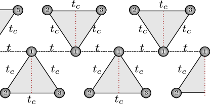
Figure 1: (Color online.) The triangular necklace lattice. The Hubbard model on this lattice has two hopping terms. The three sites within each triangle are connected by a hopping integral $t_{c}$ (solid lines), and each triangle is connected to its nearest neighbour by a hopping integral $t$ between the 1-sites only (dashed line). The maroon dotted line marks the reflection equivalent to the local parity symmetry, i.e., relabeling sites 2 and 3 on any single molecule.

In this paper, we show that the low-energy physics of the two-thirds filled Hubbard model is described, in appropriate limits, by two previously studied models. This provides simple physical pictures of the insulating phase and the behavior of the spin degrees of freedom.

Firstly, we show that in the molecular limit, $t\rightarrow 0$, the Hubbard model on triangular necklace lattice at two-thirds filling the low lying excitations of are spin excitations described by the antiferromagnetic spin-one Heisenberg chain whose ground state is in the Haldane phase. The Haldane phase is a gapped, symmetry protected topological phase with non-local string order and fractionalized edge states. Kennedy1 ; Kennedy2 ; hidden ; Haldane1 ; Haldane2

Secondly, we show that away from the molecular limit the ferromagnetic Kondo lattice model with an onsite repulsion between the itinerant electrons, which we will refer to as the ferromagnetic Hubbard-Kondo lattice model, describes the low-energy excitations of the two-thirds filled Hubbard model of the triangular necklace model. This provides a simple picture of the insulating state at two-thirds filling in the Hubbard model. It has previously been argued that both the ferromagnetic Kondo lattice model and the ferromagnetic Hubbard-Kondo lattice model have ground states in the Haldane phase.Tsunetsugu ; Garcia ; Yanagisawa

This paper is organised as follows. After a brief discussion of numerical methods in Sec. II, in section III, we solve the model for the $U=t=0$, and transform the Hamiltonian into the eigenbasis of the $U=t=0$ solution. This is a crucial conceptual step in the derivation of effective Hamiltonians that follows. We also discuss the symmetries of the full Hamiltonian focusing on the ‘local parity’ symmetry, that is a key ingredient in localizing the spins in the effective ferromagnetic Hubbard-Kondo lattice model. In Sec. IV we take recourse to second order perturbation theory and demonstrate that low lying spectrum of the Hubbard model on the triangular lattice corresponds to the two site spin-one Heisenberg model. Finally in Sec. V, we show that the model reduces to the ferromagnetic Hubbard-Kondo lattice model at half filling.

II Methods: Density matrix renormalization group

Although the central results presented here are analytical it is useful to compare these with numerical calculations to explore the parameter ranges where various approximations are valid. To do so, we employ DMRGWhite93 implemented using the matrix product states (MPS) ansatz Schollwouck and SU(2) symmetry Ian07 using the ‘MPS toolkit’ and keeping up to $\chi=1000$ states. We consider both dimers (six sites) and extended chains (120 sites or 40 molecules). All calculations are performed at at two-thirds filling (four electrons per molecule).

For dimers there are eight electrons on six sites there are $C^{12}_{8}=495$ states, where $C^{n}_{k}$ is the binomial coefficient associated with choosing $k$ objects from a set of $n$. Therefore, for dimers, we are able to retain all of the physical states and the DMRG exactly diagonalizes the Hamiltonian.

III Molecular limit ($t\rightarrow 0$)

III.1 Molecular orbital theory ($U=0$)

The molecular limit, $t\rightarrow 0$, of Hamiltonian (1) plays an important role in understanding the low-energy physics of this model. This is analogous to the role of the atomic limit in the Mott insulating phase of the half filled Hubbard model. However, the internal structure of the ‘molecule’ (three site cluster) means that the molecular limit is not as straightforward as the atomic limit. When $U=t=0$, Hamiltonian (1) reduces to the tight binding model on uncoupled triangular molecules:

$$\hat{\cal H}=-t_{c}\sum_{i}\sum_{\alpha\neq\beta,\sigma}\hat{c}^{{\dagger}}_{i\alpha\sigma}\hat{c}_{i\beta\sigma}.$$ (2)

It is straightforward to solve this Hamiltonian for the $i^{\textrm{th}}$ molecule and one finds three orbitals with energies $\varepsilon_{A_{+}}=-2t_{c}$, $\varepsilon_{E_{-}}=\varepsilon_{E_{+}}=t_{c}$. The corresponding wavefunctions, sketched in Fig. 2, are given by

$$\hat{c}^{\dagger}_{iA_{+}\sigma}|0\rangle \equiv \frac{1}{\sqrt{3}}(\hat{c}^{\dagger}_{i1\sigma}+\hat{c}^{\dagger}_{i2\sigma}+\hat{c}^{\dagger}_{i3\sigma})|0\rangle,$$ (3a)

$$\hat{c}^{\dagger}_{iE_{-}\sigma}|0\rangle \equiv \frac{1}{\sqrt{2}}(\hat{c}^{\dagger}_{i2\sigma}-\hat{c}^{\dagger}_{i3\sigma})|0\rangle,$$ (3b)

and

$$\hat{c}^{\dagger}_{iE_{+}\sigma}|0\rangle \equiv \frac{1}{\sqrt{6}}(2\hat{c}^{\dagger}_{i1\sigma}-\hat{c}^{\dagger}_{i2\sigma}-\hat{c}^{\dagger}_{i3\sigma})|0\rangle,$$ (3c)

where $|0\rangle$ is the vacuum state. We will refer to $\{\hat{c}^{\dagger}_{iA_{+}\sigma}|0\rangle,\hat{c}^{\dagger}_{iE_{+}\sigma}|0\rangle,\hat{c}^{\dagger}_{iE_{-}\sigma}|0\rangle\}$ as the molecular orbital basis and $\{\hat{c}^{\dagger}_{i1\sigma}|0\rangle,\hat{c}^{\dagger}_{2\sigma}|0\rangle,\hat{c}^{\dagger}_{i3\sigma}|0\rangle\}$ as the atomic orbital basis. The molecular orbitals are labelled based on the C₃ symmetry of an isolated molecule and the parity of the wavefunction under exchange of sites 2 and 3 on any individual molecule which remains a symmetry of the Hamiltonian even for $t\neq 0$, alternatively this transformation can be thought of as reflection through the maroon dotted lines in Figs. 1 and 2. Henceforth, we will refer to the latter symmetry as local parity.

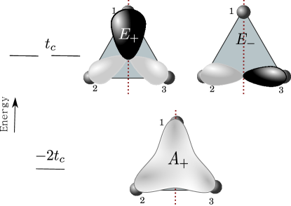
Figure 2: (Color online.) Sketches of the molecular orbitals for $t_{c}>0$. The different colors on the orbitals imply different phases of the electron wavefunction. The orbitals $A_{+}$ and $E_{+}$ have even parity under relabelling of sites 2 and 3, whereas $E_{-}$ has odd parity. Relabeling sites 2 and 3 is equivalent to reflecting (the $i^{\textrm{th}}$ molecule only) about the vertical maroon dotted line, which is also marked in Fig. 1.

For $n=4$ and $t_{c}>0$, which are the relevant parameters of Mo₃S₇(dmit)₃, the ground state of the non-interacting ($U=0$) molecular limit corresponds to a filled $A_{+}$ orbital and two electrons shared between the two $E$ orbitals (i.e., the ground state is $C^{4}_{2}=6$-fold degenerate). For $t_{c}<0$ and $n=4$, the ground state corresponds to filled $E$ orbitals and an empty $A_{+}$ orbital.

III.2 Interactions in the molecular orbital basis

We will see below that it is helpful to transform the Hamiltonian into the basis of the molecular orbitals. After this transformation the Hamiltonian Eq. (1) can be rewritten in the form

$$\hat{\mathcal{H}}=\hat{\mathcal{H}}_{\textrm{m}}+\hat{\mathcal{H}}_{t},$$ (4)

where

$$\hat{\mathcal{H}}_{t}=\sum_{imn\sigma}\hat{c}^{{\dagger}}_{im\sigma}T_{mn}\hat{c}_{(i+1)n\sigma}+H.c.,$$ (5)

$m,n\in\{A_{+},E_{+},E_{-}\}$, $T_{mn}$ is the intermolecular hopping matrix with matrix elements $T_{A_{+}A_{+}}=-t/3$, $T_{A_{+}E_{+}}=T_{E_{+}A_{+}}=-\sqrt{2}t/{3}$, and $T_{E_{+}E_{+}}=-{2}t/{3}$. It can be seen from Eq. (3b) that $E_{-}$ orbitals has no weight on site $|1\rangle$, so $T_{E_{-}m}=0$ for any $m$. However, more pertinently, this is a direct consequence of the local parity symmetry (see Sec. III.4).

$$\hat{\cal H}_{\textrm{m}}=\hat{\cal H}_{1}+\hat{\cal H}_{2}+\hat{\cal H}_{3},$$ (6)

where, $\hat{\cal H}_{n}$ describes the interactions involving $n$ orbitals on a single molecule.

$$\hat{\cal H}_{1}=\sum_{im\sigma}\varepsilon_{m}\hat{c}^{{\dagger}}_{im\sigma}\hat{c}_{im\sigma}+U_{m}n_{im\uparrow}n_{im\downarrow},$$ (7)

where $U_{A_{+}}=U/3$ and $U_{E_{-}}=U_{E_{+}}=U/2$ .

$$\hat{\cal H}_{2}=\sum_{m\neq n}\left[J_{mn}\sum_{i}\hat{\bf S}_{im}\cdot\hat{\bf S}_{in}+V_{mn}\sum_{i\sigma\sigma^{\prime}}n_{im\sigma}n_{in\sigma^{\prime}}+P_{mn}\sum_{i}\hat{c}^{{\dagger}}_{im\uparrow}\hat{c}^{{\dagger}}_{im\downarrow}\hat{c}_{in\uparrow}\hat{c}_{in\downarrow}+X_{mn}\sum_{i\sigma}\left(n_{im\sigma}\hat{c}^{{\dagger}}_{im\bar{\sigma}}\hat{c}_{in\bar{\sigma}}+H.c.\right)\right],$$ (8)

where $\hat{\bf S}_{im}=\hat{c}^{{\dagger}}_{im\alpha}{\bm{\sigma}}_{\alpha\beta}\hat{c}_{im\beta}$, ${\bm{\sigma}}$ is the vector of Pauli matrices, $J_{mn}$ is the ferromagnetic interorbital exchange interaction, $V_{mn}$ is the interorbital Coulomb interaction, $P_{nm}$ is a two electron interorbital hopping, and $X_{mn}$ is a correlated interorbital hopping. The Hermiticity of the Hamiltonian requires that $J_{mn}=J_{nm}$, $V_{mn}=V_{nm}$, and $P_{mn}=P_{nm}$, the C₃ symmetry of the isolated molecule requires that $J_{mE_{+}}=J_{mE_{-}}$, $V_{mE_{+}}=V_{mE_{-}}$, $P_{mE_{+}}=P_{mE_{-}}$; and the local parity symmetry requires that $X_{mE_{-}}=X_{E_{-}m}=0$. Explicitly transforming from the atomic orbital basis to the molecular orbital basis reveals that the remaining undefined parameters are $J_{A_{+}E_{+}}=-U/3$, $J_{E_{+}E_{-}}=-U/6$, $V_{A_{+}E_{+}}=U/12$, $V_{E_{+}E_{-}}=U/24$, $P_{A_{+}E_{+}}=-U/3$, $P_{E_{+}E_{-}}=-U/6$, $X_{A_{+}E_{+}}=0$ and $X_{E_{+}A_{+}}=U/3\sqrt{2}$. The problem of determining such parameters for first principles in molecular solids has recently been discussed extensively.Nakamura ; Laura ; Scriven1 ; Scriven2

$$\hat{\cal H}_{3} = \frac{U}{3\sqrt{2}}\sum_{i\sigma}\left(\hat{c}^{{\dagger}}_{iA_{+}\sigma}\hat{c}^{{\dagger}}_{iE_{+}\overline{\sigma}}\hat{c}_{iE_{-}\sigma}\hat{c}_{iE_{-}\overline{\sigma}}+H.c\right)+\frac{U}{3\sqrt{2}}\sum_{i\sigma}\left(\hat{c}^{{\dagger}}_{iE_{-}\sigma}\hat{c}_{iE_{-}\overline{\sigma}}\hat{c}^{{\dagger}}_{iE_{+}\overline{\sigma}}\hat{c}_{iA_{+}\sigma}+H.c.\right)$$ (9)

$$-\frac{U}{3\sqrt{2}}\sum_{i\sigma}\left(n_{iE_{-}\sigma}\hat{c}^{{\dagger}}_{iE_{+}\overline{\sigma}}\hat{c}_{iA_{+}\overline{\sigma}}+H.c.\right)$$

Note that $\hat{\cal H}_{\textrm{m}}$ is the Hubbard model on a triangle, which can be solved exactly. The ground state of this model at two-thirds filling for $t_{c}>0$ is a triplet with energy $-2t_{c}+U$. The (degenerate) ground state wavefunctions for the $i^{\textrm{th}}$ monomer are therefore

$$|\phi_{i}^{\Uparrow}\rangle = |A_{+}^{\uparrow\downarrow},E_{-}^{\uparrow},E_{+}^{\uparrow}\rangle=\hat{c}^{{\dagger}}_{iA_{+}\uparrow}\hat{c}^{{\dagger}}_{iA_{+}\downarrow}\hat{c}^{{\dagger}}_{iE_{-}\uparrow}\hat{c}^{{\dagger}}_{iE_{+}\downarrow}|0\rangle$$ (10a)

$$|\phi_{{i}}^{\Downarrow}\rangle = |A_{+}^{\uparrow\downarrow},E_{-}^{\downarrow},E_{+}^{\downarrow}\rangle=\hat{c}^{{\dagger}}_{iA_{+}\uparrow}\hat{c}^{{\dagger}}_{iA_{+}\downarrow}\hat{c}^{{\dagger}}_{iE_{-}\downarrow}\hat{c}^{{\dagger}}_{iE_{+}\uparrow}|0\rangle$$ (10b)

$$|\phi_{{i}}^{0}\rangle = \frac{1}{\sqrt{2}}\left(|A_{+}^{\uparrow\downarrow},E_{-}^{\uparrow},E_{+}^{\downarrow}\rangle+|A_{+}^{\uparrow\downarrow},E_{-}^{\downarrow},E_{+}^{\uparrow}\rangle\right)=\frac{1}{\sqrt{2}}\left(\hat{c}^{{\dagger}}_{iA_{+}\uparrow}\hat{c}^{{\dagger}}_{iA_{+}\downarrow}\hat{c}^{{\dagger}}_{iE_{-}\uparrow}\hat{c}^{{\dagger}}_{iE_{+}\uparrow}+\hat{c}^{{\dagger}}_{iA_{+\uparrow}}\hat{c}^{{\dagger}}_{iA_{+}\downarrow}\hat{c}^{{\dagger}}_{iE_{-}\downarrow}\hat{c}^{{\dagger}}_{iE_{+}\downarrow}\right)|0\rangle,$$ (10c)

where the superscripts on the terms between the two equality signs label the spin(s) of the electron(s) in that orbital. For two-thirds filling, i.e., four electrons in three orbitals, one of orbitals will be doubly occupied. It can be seen from the ground states that for $t_{c},U>0$ and $t=0$, the $A_{+}$ orbital continues to be doubly occupied, as in the case of $U=0$. This is not unexpected as $U_{A_{+}}=U/3<U_{E_{+}}=U_{E_{-}}=U/2$. The remaining two electrons occupy $E_{+}$ and $E_{-}$ orbitals with one electron each respectively as the intraorbital Coulomb interaction for the $E$ orbitals is greater than the competing interorbital interaction $V_{E_{+}E_{-}}=U/12$. The interaction $J_{E_{+}E_{-}}$ lowers the energy of the triplet relative to that of the singlet. Thus in the molecular limit the Hubbard model on the triangular necklace lattice consists of spin triplet molecules.

III.3 Nagaoka’a theorem and Hund’s rules

The above result, that the grounds state of an isolated triangle is a triplet, can be understood in terms of two physical effects that are usually regarded as entirely separate pieces of physics: Nagaoka’s theorem and Hund’s rules. The most general formulation of Nagaoka’s theorem Tasaki states that for $U=\infty$ the ground state of the Hubbard model with $N-1$ electron on $N$ lattice sites has the maximum possible spin, $S=(N-1)/2$, if all of the intersite hopping integrals are negative.foot-sign To make connection with this result we must return to the atomic orbital basis and make a particle-hole transformation, $\hat{h}_{i\alpha\sigma}=\hat{c}^{\dagger}_{i\alpha\sigma}$. The Hamiltonian for $t=0$ and $t_{c}>0$ is then

$$\hat{\cal H} = -(-t_{c})\sum_{i,\alpha\neq\beta,\sigma}\hat{h}^{\dagger}_{i\alpha\sigma}\hat{h}_{i\beta\sigma}$$ (11)

$$+U\sum_{i\alpha}\hat{h}^{\dagger}_{i\alpha\uparrow}\hat{h}_{i\alpha\uparrow}\hat{h}^{\dagger}_{i\alpha\downarrow}\hat{h}_{i\alpha\downarrow}+U.$$

We remove the trivial term by shifting the zero of energy: $\hat{\cal H}\rightarrow\hat{\cal H}-U.$ We then regain a Hubbard model with 2 fermions on 3 sites and all hopping integrals are negative. Thus Nagaoka’s theorem implies an $S=1$ ground state when $U\rightarrow\infty$, as we found explicitly above. Of course, on this finite lattice the triplet groundstate is found even away from $U=\infty$, which is not guaranteed by Nagaoka’s theorem. Furthermore, Nagaoka’s theorem states that the ground state wavefunction contains only positive coefficients when written in the natural real-space many-body basis.Tasaki Returning to the molecular orbital basis and working with electrons rather than holes, this statement is equivalent to the prediction that the $A_{+}$ orbital will be doubly occupied, as indeed we found explicitly above. In the molecular orbital basis it is clear that $J_{E_{+}E_{-}}$ plays a key role in stabilizing the Nagaoka state.

If we accept that the $A_{+}$ orbital will be doubly occupied, then, the triplet ground state is what one would expect from the molecular Hund’s rules applied to the $E$ orbital subspace. Note however, that we do not include an explicit Hund’s rule coupling, rather one simply finds $J_{E_{+}E_{-}}<0$ on transforming into the molecular orbital basis. Indeed, the connection to Hund’s rules goes beyond the maximization of $S$ within the $E$ manifold. One can rewrite the Hamiltonian in terms of ‘molecular Kanamori parameters’ $\tilde{U},\tilde{U}^{\prime},\tilde{J}$ and $\tilde{J}^{\prime}$ (cf. Eq. (35) of Ref. Hotta, ). In which case the electron-electron interactions within the $E$ manifold of the $i^{\textrm{th}}$ molecule are given by

$${\cal H}^{E}_{i} = \tilde{U}\sum_{\nu}\hat{n}_{i\nu\uparrow}\hat{n}_{i\nu\downarrow}+\tilde{U}^{\prime}\sum_{\sigma\sigma^{\prime}}\hat{n}_{iE_{+}\sigma}\hat{n}_{iE_{-}\sigma^{\prime}}$$ (12)

$$+\tilde{J}\sum_{\sigma\sigma^{\prime}}\hat{c}^{\dagger}_{iE_{+}\sigma}\hat{c}^{\dagger}_{iE_{-}\sigma^{\prime}}\hat{c}_{iE_{+}\sigma^{\prime}}\hat{c}_{iE_{-}\sigma}$$

$$+\tilde{J}^{\prime}\left(\hat{c}^{\dagger}_{iE_{+}\uparrow}\hat{c}^{\dagger}_{iE_{+}\downarrow}\hat{c}_{iE_{-}\downarrow}\hat{c}_{iE_{-}\uparrow}+H.c.\right).$$

On writing Eq. (8) in this form one finds that $\tilde{U}=U/2$ and $\tilde{U}^{\prime}=\tilde{J}=\tilde{J}^{\prime}=U/6$. This satisfies two important constraints, which the Kanamori parameters are required to respect: (i) $\tilde{J}=\tilde{J}^{\prime}$ and (ii) $\tilde{U}=\tilde{U}^{\prime}+\tilde{J}+\tilde{J}^{\prime}$. In terms of the parameters used elsewhere in this paper these constraints correspond to (i) $J_{E_{+}E_{-}}=P_{E_{+}E_{-}}$ and (ii) $U_{E_{+}}=U_{E_{-}}=2V_{E_{+}E_{-}}-\frac{3}{2}J_{E_{+}E_{-}}-P_{E_{+}E_{-}}$.

Furthermore, it is the interactions described by the Kanamori parameters that are responsible for Hund’s rules in the $e_{g}$ manifold of a $d$-electron systems.Hotta Therefore, in transforming to the molecular orbital basis, we have explicitly derived Hund’s rules for the $E$ manifold of the molecule.

Therefore, it is clear that, in this system at least, Hund’s rules and Nagaoka’s theorem result from the same underlying physics. It is natural to speculate that this connection may be more general.

III.4 Local parity

It is important to note that, even if we restrict the relabeling of sites 2 and 3 to a single molecule, the local parity (defined in Sec. III.1) is a symmetry of the Hubbard model for all $t,U$. Thus, all eigenstates, and in particular the ground state, have a definite local parity on every site individually. For example, in Sec. III.1 we saw that for $t=U=0$ and $t_{c}>0$ there are six degenerate ground states on each molecule, which we can label

$$|\alpha_{+}\rangle = |A_{+}^{\uparrow\downarrow},E_{-}^{\uparrow\downarrow},E_{+}^{0}\rangle,$$ (13a)

$$|\beta_{-}\rangle = |A_{+}^{\uparrow\downarrow},E_{-}^{\uparrow},E_{+}^{\uparrow}\rangle,$$ (13b)

$$|\gamma_{-}\rangle = |A_{+}^{\uparrow\downarrow},E_{-}^{\uparrow},E_{+}^{\downarrow}\rangle,$$ (13c)

$$|\delta_{-}\rangle = |A_{+}^{\uparrow\downarrow},E_{-}^{\downarrow},E_{+}^{\uparrow}\rangle,$$ (13d)

$$|\epsilon_{-}\rangle = |A_{+}^{\uparrow\downarrow},E_{-}^{\downarrow},E_{+}^{\downarrow}\rangle,$$ (13e)

and

$$|\zeta_{+}\rangle = |A_{+}^{\uparrow\downarrow},E_{-}^{0},E_{+}^{\uparrow\downarrow}\rangle.$$ (13f)

It is clear that $|\alpha_{+}\rangle$ and $|\zeta_{+}\rangle$ have even parity and $|\beta_{-}\rangle$, $|\gamma_{-}\rangle$, $|\delta_{-}\rangle$, and $|\epsilon_{-}\rangle$ have odd parity as the only molecular orbital with odd local parity with respect to the $i^{\textrm{th}}$ molecule is $\hat{c}_{iE_{-}\sigma}^{\dagger}|0\rangle$. This means that arbitrary perturbations that respect the local parity symmetry may mix $|\alpha_{+}\rangle$ with $|\zeta_{+}\rangle$ or any of the set $|\beta_{-}\rangle$, $|\gamma_{-}\rangle$, $|\delta_{-}\rangle$, and $|\epsilon_{-}\rangle$, but perturbations that respect the local parity symmetry will not mix even parity states with odd parity states.

In particular, as non-zero $t$ and non-zero $U$ do not break local parity symmetry this means that even away from the $t=U=0$ limit the local eigenstates have a definite local parity with respect to each molecule individually. This is turn, implies that in any state the occupation number of the $E_{-}$ orbital is conserved modulo two (individually) on every molecule (as changes by $\pm 1$ result in a change in the local parity). In particular when $n_{iE_{-}}\equiv\sum_{\sigma}n_{iE_{-}\sigma}=1$ the electron is localized on the $i^{\textrm{th}}$ molecule as long as there is no phase transition.

It is clear from Eqs. (7-9) and the fact that $T_{mE_{-}}=0$ for all $m$ that the explicit form of $\hat{\cal H}$ given in Sec. III.2 conserves $\hat{n}_{iE-}$ modulo two for all $i$.

IV Spin-One Heisenberg Chain

It is well known that in the atomic limit, $U\gg t$, the low-energy physics of the half-filled Hubbard model is described by the spin-half antiferromagnetic Heisenberg model. This result can be derived via second-order perturbation theory.Auerbach In the same spirit, we now show that the low energy physics of two thirds filled Hubbard model on the triangular necklace model is described by an effective spin-one Heisenberg model in the molecular limit, $t\ll t_{c},U$.

We take $\hat{\mathcal{H}}_{\textrm{m}}$ (cf. Eq. (6)) as the zeroth order Hamiltonian and include $\hat{\mathcal{H}_{t}}$ (cf. Eq. (5)) perturbatively. As we will only work to second order we may limit our calculation to a system composed of two molecules without loss of generality. The ground state of $\hat{\mathcal{H}}_{\textrm{m}}$ on two molecules (i.e., a dimer) has bare energy $E^{(0)}=-4t_{c}+2U$ and is nine-fold degenerate. As the total spin of the two molecules is a good quantum number of the full Hamiltonian, $\hat{\mathcal{H}}$, it is helpful to consider each spin sector independently. At various points in the derivation we will need to relate the results of the perturbation theory to the exact solution of the two-site spin-one Heisenberg model; for convenience, we summarize this in Fig. 3.

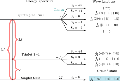
Figure 3: Spectrum of the two site Haldane model, $\hat{\cal H}=J\hat{\bf S}_{1}\cdot\hat{\bf S}_{1}$. Here, the local basis on each site is represented by $|0\rangle$, $|\uparrow\rangle$ and $|\downarrow\rangle$ corresponding to $S_{z}$=0, $S_{z}$=1 and $S_{z}$=-1 respectively.

IV.1 Singlet sector

The $S=0$ member of the ground state manifold of $\hat{\mathcal{H}}_{\textrm{m}}$ on the dimer consisting of the $i^{\textrm{th}}$ and $j^{\textrm{th}}$ monomers, where $j=i\pm 1$, is

$$|\phi_{ij}^{0}\rangle=\frac{1}{\sqrt{3}}\left(|\phi^{\Uparrow}_{i}\rangle\otimes|\phi^{\Downarrow}_{j}\rangle+|\phi^{\Downarrow}_{i}\rangle\otimes|\phi^{\Uparrow}_{j}\rangle-|\phi^{0}_{i}\rangle\otimes|\phi^{0}_{j}\rangle\right).$$

(14)

Note that it has same form as the singlet ground state of a two site spin-one antiferromagnetic Heisenberg model (cf. Fig. 3). To second order in $\hat{\mathcal{H}}_{t}$, the energy of the singlet state is

$$E^{(2)}_{S=0} = E^{(0)}+\sum_{m_{0}}\frac{\langle\phi_{ij}^{0}|\hat{\mathcal{H}}_{t}|m_{0}\rangle\langle m_{0}|\hat{\mathcal{H}}_{t}|\phi_{ij}^{0}\rangle}{E^{(0)}-E_{m_{0}}}$$ (15)

$$= -4t_{c}+2U-3\sum_{n=1}^{4}\frac{4t^{2}}{9a_{n}\left(3t_{c}+\varepsilon_{n}\right)},$$

where $|m_{0}\rangle$ is the set of all possible intermediate wavefunctions which are formed by the hopping of electrons from one monomer to another, $\varepsilon_{1}=U$, and for $n>1$

$$\varepsilon_{n} = \frac{2}{3}\left[U+\xi\cos\left(\frac{\phi+2\pi n}{3}\right)\right],$$ (16)

where

$$\xi = \sqrt{U^{2}+27t_{c}^{2}},$$ (17)

and

$$\phi = \pi+\arccos\left(\left(\frac{U}{\xi}\right)^{3}\right).$$ (18)

$a_{1}=3$ and for $n>1$

$$a_{n} = 2|\alpha_{n}|^{2}+|\beta_{n}|^{2}+1,$$ (19)

where

$$\alpha_{n} = \frac{-12t_{c}^{2}U-9t_{c}^{2}\varepsilon_{n}+U^{2}\varepsilon_{n}-2U\varepsilon_{n}^{2}+\varepsilon_{n}^{3}}{\sqrt{2}(U-\varepsilon_{n})(3t_{c}+U-\varepsilon_{n})\varepsilon_{n}}$$ (20)

and

$$\beta_{n} = \frac{U-3t_{c}-\varepsilon_{n}}{U+3t_{c}-\varepsilon_{n}}.$$ (21)

In Fig. 4, we plot the difference in the energy, $\delta E_{S=0}=|E_{S=0}^{(2)}-E^{\textrm{DMRG}}_{S=0}|$, between the lowest energy singlet wavefunctions obtained from perturbation theory and the DMRG ground state for the Hubbard model on the two triangular dimer, which is a singlet. It can be seen that, even for relatively small $U$, the error in the energy obtained is of the $\mathcal{O}(10^{-3}$) for $t/t_{c}\lesssim 0.25$ and $\mathcal{O}(10^{-2}$) for $t/t_{c}\lesssim 0.5$. Thus, for the dimer, the perturbation theory gives remarkably good agreement with the DMRG results in the singlet sector.

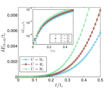
Figure 4: The difference in energy $\delta E_{S=0}=|E_{S=0}^{(2)}-E^{\textrm{DMRG}}_{S=0}|$ of singlet wavefunctions obtained from second order perturbation theory, $E_{S=0}^{(2)}$ and DMRG, $E^{\textrm{DMRG}}_{S=0}$, for selected values of $U$. Excellent agreement between the perturbation theory and the exact DMRG is found even for quite large $t$. The inset shows the same data on a semi-logarithmic scale.

IV.2 Triplet sector

As spin is a good quantum number of the full Hamiltonian, we know that, while the perturbation may lift the degeneracy of the singlet, triplet and quintuplet, it will not split the triplet (or quintuplet). Therefore, it suffices to consider only one of the unperturbed triplet wavefunctions of the dimer. A convenient choice (cf. Fig. 3) is

$$|\phi_{ij}^{1}\rangle=\frac{1}{\sqrt{2}}\left(-|\phi^{\Uparrow}_{i}\rangle\otimes|\phi^{\Downarrow}_{j}\rangle+|\phi^{\Downarrow}_{i}\rangle\otimes|\phi^{\Uparrow}_{j}\rangle\right).$$ (22)

To second order in $\hat{\mathcal{H}}_{t}$, the energy of the triplet states is

$$E_{S=1}^{(2)} = E^{(0)}-\frac{4t^{2}}{81t_{c}}-2\sum_{n=1}^{4}\frac{4t^{2}}{9a_{n}\left(3t_{c}+\varepsilon_{n}\right)}$$

Fig. 5 shows the of the energy difference, $\delta E_{S=1}=|E_{S=1}^{(2)}-E^{\textrm{DMRG}}_{S=1}|$, between the second order perturbation theory and the lowest energy triplet state found in the DMRG solution for the Hubbard model on a triangular necklace dimer. It can be seen that, as for the singlet case, the analytical calculation agrees well with the numerical results.

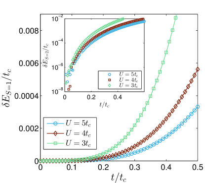
Figure 5: The difference in the energy of the triplet wavefunction $\delta E_{S=1}$ obtained using perturbation theory and numerically using DMRG for $U=3tc,\;4t_{c}\;$ and $5t_{c}$ as a function of perturbation $t/t_{c}$. Excellent agreement between the perturbation theory and the exact DMRG is found even for quite large $t$. The inset shows the same data on a semi-logarithmic scale.

IV.3 Quintuplet sector

Finally, we consider the effect of perturbation on one of the $S=2$ sector. It is convenient to consider the unperturbed state

$$|\phi_{ij}^{2}\rangle=|\phi^{\Uparrow}_{i}\rangle\otimes|\phi^{\Uparrow}_{j}\rangle$$ (24)

To second order in $\hat{\mathcal{H}}_{t}$, the energy of the quintuplet states is

$$E_{S=2}^{(2)}=E^{(0)}-\frac{4t^{2}}{27t_{c}}.$$ (25)

We will see below that this simple form for the quintuplet energy is a consequence of the Pauli blockade.

Fig. 6 shows difference in the energies, $\delta E_{S=2}=|E_{S=2}^{(2)}-E^{\textrm{DMRG}}_{S=2}|$, of the lowest quintuplet solutions found from second order perturbation theory and from DMRG. As for $S=0$ and $S=1$, the error in the perturbation theory is small: indeed for the quintuplet the errors are two orders of magnitude smaller than those for the singlet or triplet sectors. Yet the most striking feature of the plot is that the the error in the energy is independent of $U$. This is a consequence of Pauli blockade and is simple to understand in the molecular orbital basis. In the unperturbed quintuplet state described by Eq. (24) each molecule contains three spin-up electrons (one in each MO) and one spin-down (in the $A_{+}$ orbital). Therefore, to second order, the only possible corrections involve the spin-down electron virtually hopping into the $E_{+}$ orbital (recall that the local parity symmetry forbids hopping into the $E_{-}$ orbital). As these fluctuations do not change the total number of doubly occupied sites (indeed no processes can change the number of doubly occupied sites as we have six spin-up and two spin-down electrons in six orbitals and there are no spin flip terms in the perturbing Hamiltonian, $\hat{\mathcal{H}}_{t}$) $U$ cannot enter into the correction to the quintuplet energy, $E_{S=2}^{(2)}-E^{(0)}$. This results in the simple form of Eq. (25). Indeed, the only higher order corrections on the dimer involve both down electrons taking part in such virtual process. This explains why both $E_{S=2}^{(2)}-E^{(0)}$ and $\delta E_{S=2}$, are independent of $U$ and why the perturbation theory is so accurate.

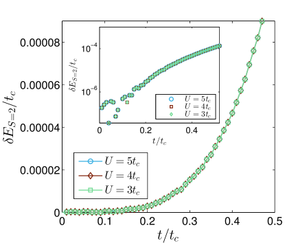
Figure 6: The difference in the energy of the quintuplet wavefunction $\delta E_{S=2}^{2}$ obtained using perturbation theory and from DMRG for selected values of $U$. The error in the perturbation theory is two orders of magnitude smaller than for the singlet (Fig. 4) or triplet (Fig. 4) sectors. Furthermore, the error is independent of $U$. Both of these effects are to due to the Pauli blockade. The inset shows the same data on a semi-logarithmic scale.

IV.4 Calculation of interaction strength, $J_{s}$

With the above results in hand, we can now make explicit connection to the Heisenberg model. The singlet-triplet energy gap is

$$J_{s}\equiv E^{2}_{S=1}-E^{2}_{S=0}=\sum_{n=0}^{4}\frac{4t^{2}}{9a_{n}\left(3t_{c}+\varepsilon_{n}\right)}$$ (26)

where we have defined $\varepsilon_{0}=0$ and $a_{0}=-3$ for notational convenience. Similarly, we can calculate energy difference between the singlet and quadruplet and that of quintuplet and triplet. We find that

$$E^{2}_{S=2}-E^{2}_{S=1}=2J_{s}$$ (27)

$$E^{2}_{S=2}-E^{2}_{S=0}=3J_{s}$$ (28)

The above spectrum precisely maps onto that of spin-1 Heisenberg dimer, summarised in Fig. 3. A comparison of the interaction strength obtained from perturbation theory and DMRG is shown in Fig. 7. The estimation of the interaction strength $J_{s}$ calculated using perturbation theory agrees well with the DMRG calculation in the limit $U,\;t_{c}\gg t$ where one would expect the perturbation theory to hold.

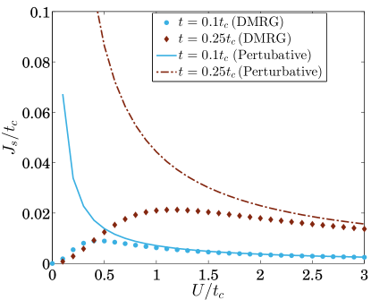
Figure 7: Comparison of the interaction strength $J_{s}\equiv E_{S=1}-E_{S=0}=(E_{S=2}-E_{S=1})/2=(E_{S=2}-E_{S=0})/3$ as function of $U$ obtained from perturbation theory and from DMRG calculations for the Hubbard model on the six-site dimer.

For DMRG calculations on large systems with open boundary conditions we find that the ground state is a singlet, but there is a triplet state at a vanishingly small energy above the ground state. These two states are separated from all other states by a much larger spin gap. This is consistent with the $D_{2}\cong Z_{2}\times Z_{2}$ degeneracy expected for the Haldane phase.Kennedy2 ; Kennedy1 This can be understood as arising from the the emergent spin-1/2 edge states, which have an interaction that becomes exponentially small as the system is taken into the thermodynamic limit.Ken In Fig. 8 we plot the spin gap, $\Delta_{s}=E_{2}(4L)-E_{0}(4L)$ where $E_{S}(N_{e})$ is the energy of the lowest energy eigenstate for $N_{e}$ electrons in the spin-$S$ subspace, calculated from DMRG for $L=40$ molecules (120 sites), scaled by $J_{s}$ for a range of parameters. We find, as expected, that in the strong coupling molecular limit the value of $\Delta_{s}/J_{s}$ is comparable to that found for the spin-1 Heisenberg model.White Indeed the agreement is remarkably good given the additional numerical difficulties of dealing with a fermionic system such as the Hubbard model.

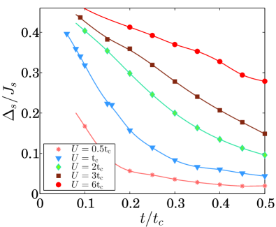
Figure 8: The spin gap, $\Delta_{s}$, for $L=40$ molecules is consistent with the expected size of the Haldane gap expected from the magnitude of the superexchange interaction $J_{s}$. For comparison the Haldane spin gap for the spin-1 Heisenberg model is $0.41J_{s}$ White . Curves are guides to the eye.

Thus we conclude that the spin-one antiferromagnetic Heisenberg model with interaction strength $J_{s}$ provides an effective low-energy theory of the two-thirds filled Hubbard model on the triangular necklace lattice in the limit $U,\;t_{c}\gg t$. It follows that, in this limit, the Hubbard model will be in the Haldane phase.Haldane1 ; Haldane2 However, this model does not give any insight into what happens outside of this limit, when one expects charge fluctuations to become important. Furthermore, this limit gives no insight into why the two-thrids filled Hubbard model on the triangular necklace model is insulating at finite $U$.

V Ferromagnetic Hubbard-Kondo lattice model

In this section we show that, if the $A_{+}$ orbitals are projected out of the low-energy model we are left with a Hubbard-Kondo lattice model with the itinerant $E_{+}$ electrons ferromagnetically coupled to localised spins in the $E_{-}$ orbitals.

V.1 Projection of the Hamiltonian onto the $\hat{n}_{iE_{-}}=1$ subspace

We have seen above that in the molecular limit with $U=\infty$, there is exactly one electron in every $E_{-}$ orbital. Furthermore, we have seen that the local parity symmetry on every molecule is a conserved quantity. Therefore, the occupation of the $E_{-}$ orbital is conserved modulo two. This means that, if we start from the strong coupling molecular limit and gradually reduce $U$ and increase $t$ one should expect the $E_{-}$ orbitals to remain singularly occupied unless or until there is a phase transition, where the occupation number of the $E_{-}$ orbitals may change non-adiabatically. This can occur because the absence of adiabatic continuity at a phase transition allows energy levels with different parities to cross.

In Fig. 9, we plot the occupations of the molecular orbitals for the Hubbard model on 120 sites (40 molecules) obtained from DMRG calculations. In Fig. 10 we plot the variance in these occupations. We can see that for all $U$, $n_{A_{+}}\simeq 2$, $n_{E_{-}}=1$ and $n_{E_{+}}\simeq 1$. A striking feature of the above plot is that the occupancy of the $E_{-}$ orbital is strictly one. Furthermore, there are no charge fluctuations in $E_{-}$ orbital (cf. Fig. 10). We have seen above that there is exactly one electron in each $E_{-}$ orbital for $U\rightarrow\infty$ and that, provided there is not phase transition this remains the case for smaller $U$. Therefore the numerical finding that $n_{E_{-}}=1$ is consistent with the previous findingJanani that there is no phase transition, at least down to a very small $U$ where numerics become extremely challenging, as $U$ is reduced on the triangular necklace model.

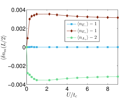
Figure 9: The deviation in the filling of the molecular orbitals filling from that expected in the $U=\infty$ molecular limit.

Therefore, we conclude that, at least in a large region of (and probably throughout) the phase diagram $\hat{n}_{iE_{-}}=1$ on all molecules and one can project the Hamiltonian onto the subspace with exactly one electron in $E_{-}$ orbital on every molecule without introducing an approximation. The projection operator onto $\hat{n}_{iE_{-}}=1$ is

$$\hat{P}_{1}=\left[1-\hat{n}_{iE_{-\uparrow}}\hat{n}_{iE_{-\downarrow}}\right]\left[\hat{n}_{iE_{-\uparrow}}+\hat{n}_{iE_{-\downarrow}}\right].$$ (29)

Under this projection the Hamiltonian $\hat{\cal H}$ yields

$$\tilde{\cal H}=\hat{P}_{1}^{{\dagger}}\hat{\cal H}\hat{P}_{1}=\hat{P}_{1}^{\dagger}\left(\tilde{\cal H}_{t}+\tilde{\cal H}_{1}+\tilde{\cal H}_{2}+\tilde{\cal H}_{3}\right)\hat{P}_{1},$$ (30)

where,

$$\tilde{\cal H}_{t} = \sum_{\sigma}\sum_{n,m\neq E_{-}}\left(\hat{c}^{{\dagger}}_{im\sigma}T_{mn}\hat{c}_{(i+1)n\sigma}+H.c.\right),$$ (31a)

$$\tilde{\cal H}_{1} = \sum_{m\sigma}\varepsilon_{m}\hat{c}^{\dagger}_{im\sigma}\hat{c}_{im\sigma}+\sum_{m\neq E_{-}}U_{m}\hat{n}_{im\uparrow}\hat{n}_{im\downarrow},$$ (31b)

$$\tilde{\cal H}_{2} = \sum_{imn}J_{mn}\hat{\mathbf{S}}_{im}.\hat{\mathbf{S}}_{in}+\sum_{imn\sigma}V_{mn}\hat{n}_{im\sigma}\hat{n}_{in\sigma^{\prime}}$$ (31c)

$$+\sum_{i\sigma}\sum_{m,n\neq E_{-}}X_{mn}\left(\hat{n}_{im\sigma}\hat{c}^{\dagger}_{im\bar{\sigma}}\hat{c}_{in\bar{\sigma}}+H.c.\right)$$

$$+\sum_{i}\sum_{m,n\neq E_{-}}P_{mn}\hat{c}^{\dagger}_{im\uparrow}\hat{c}^{\dagger}_{im\downarrow}\hat{c}_{in\uparrow}\hat{c}_{in\downarrow},$$

and

$$\tilde{\cal H}_{3} = \frac{U}{3\sqrt{2}}\sum_{i\sigma}\left(\hat{c}^{\dagger}_{iE_{-}\sigma}\hat{c}_{iE_{-}\overline{\sigma}}\hat{c}^{\dagger}_{iE_{+}\overline{\sigma}}\hat{c}_{iA_{+}\sigma}+H.c.\right)$$ (31d)

$$-\frac{U}{3\sqrt{2}}\sum_{i\sigma}\left(\hat{n}_{iE_{-}\sigma}\hat{c}^{\dagger}_{iE_{+}\overline{\sigma}}\hat{c}_{iA_{+}\overline{\sigma}}+H.c.\right).$$

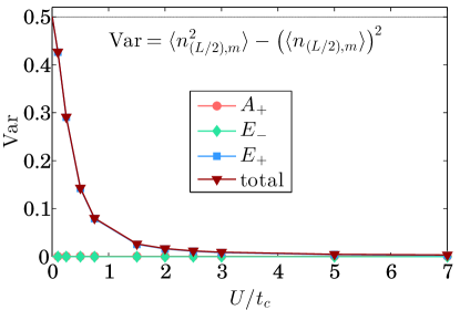
Figure 10: Charge fluctuations in different orbitals on a molecule of the chain as a function of $U$ for $t=0.1t_{c}$ using DMRG. These calculations indicate that for all values of $U$ studied there are no charge fluctuations in the $E_{-}$ orbital, as expected from symmetry when $n_{E_{-}}=1$. The charge fluctuations in $A_{+}$ is also negligible.

V.2 Projection of the Hamiltonian to $\hat{n}_{iA_{+}}=2$

In the molecular limit, i.e., as $t\rightarrow 0$ (cf. sec III.2) we found that the $A_{+}$ orbitals are doubly occupied. This is also the case in the non-interacting ($U=0$) and $U=\infty$ solutions. Away from these limits we expect this to be an approximation as this is not protected by symmetry. The DMRG calculations in Figs. 9 and 10 coincide with this expectation, but show that, for all $U$ studied, the charge transferred from the $A_{+}$ orbitals to the $E_{+}$ orbitals is negligibly small. Furthermore, because these orbitals are nearly filled, rather than, say, nearly half-filled as is the case for the $E_{+}$ orbital, one does not see large charge fluctuations in the $A_{+}$ orbital and therefore one does not expect electronic correlations in the $A_{+}$ orbitals to play an important role in determining the physics of the Hubbard model. This is borne out by the DMRG calculations (see also Fig. 10). Therefore we now further project onto the $\hat{n}_{iA_{+}}=2$ subspace via a ‘anti-Gutzwiller’ projection $\hat{P}_{\overline{G}}=\hat{n}_{A_{+}\uparrow}\hat{n}_{A_{+}\downarrow}$. On the basis of the analytical results described above we expect this approximation to work best for small $t$ and in both the limits $U\rightarrow 0$ and $U\rightarrow\infty$. It is less clear how good this approximation remains for intermediate $U$ and large $t$ where the charge fluctuations in the $A_{+}$ orbital in our DMRG calculations are largest.

Projecting the Hubbard model onto both $n_{E_{-}}=1$ and $n_{A_{+}}=2$ one finds that

$$\hat{H}_{\textrm{eff}} \equiv \hat{P}_{\overline{G}}^{{\dagger}}\hat{P}_{1}^{{\dagger}}\hat{H}\hat{P}_{1}\hat{P}_{\overline{G}}$$

$$= N\varepsilon_{E_{+}}^{*}-t^{*}\sum_{i\sigma}\left(\hat{c}^{{\dagger}}_{iE_{+}\sigma}\hat{c}_{i+1E_{+}\sigma}+H.c.\right)$$

$$+U^{*}\sum_{i}\hat{n}_{iE_{+}\uparrow}\hat{n}_{iE_{+}\downarrow}-J^{*}\sum_{i}\hat{\mathbf{S}}_{iE_{+}}\cdot\hat{\mathbf{S}}_{iE_{-}}$$

where $\varepsilon_{E_{+}}^{*}=4V_{A_{+}E_{+}}+V_{E_{+}E_{-}}+2\varepsilon_{A_{+}}+2\varepsilon_{E_{+}}+U_{A_{+}}=17U/24-2t_{c}$, $t^{*}=-T_{E_{+}E_{+}}=2t/3$, $U^{*}=U_{E_{+}}=U/2$, $J^{*}=-2J_{E_{+}E_{-}}=U/3$, and $N$ is the total number of molecules. Up to the trivial term proportional to $\varepsilon_{E_{+}}^{*}$, this is simply the Kondo lattice model with a ferromagnetic exchange interaction between the localized $E_{-}$ spins and the itinerant $E_{+}$ electrons with a on site repulsive Hubbard interaction between the $E_{+}$ electrons, i.e., the ferromagnetic Hubbard-Kondo lattice model.

The ferromagnetic Hubbard-Kondo lattice model with $S=1/2$ impurities has not been extensively studied at half-filling in one spatial dimension. A numerical study using quantum Monte Carlo (QMC), DMRG and exact diagonalization of this model for large $U^{*}$ and various dopings,Dagotto found that model has a complicated phase diagram, with a ferromagnetic phase away from half filling and incommensurate spin order near half filling. However, at half filling, the nature of the ground state is not clear, as the half filling density is not accessible to QMC due to sign problem.

The $U^{*}=0$ version of this model, i.e., the ferromagnetic Kondo lattice model has been studied in more detail for various doping. Garcia ; Tsunetsugu ; Dagotto But, again, the half-filled case has received scant attention. We are only aware of two very brief reports, Garcia ; Tsunetsugu which claim that this model is insulating, with antiferromagnetic correlations with a spin gap and has a ground state which belongs to the Haldane phase. Clearly this is correct for $J^{*}\rightarrow\infty$ in our model. Further, an investigation of a variant of the ferromagnetic Hubbard-Kondo lattice model with additional interactions,Malvezzi found that onsite Coulomb interactions does not change the phase of the model qualitatively. Yanagisawa and Shimoi Yanagisawa proved that for a bipartite lattice with $U^{*}>J^{*}/4$ the ground state of the ferromagnetic Hubbard-Kondo lattice model is a singlet. This is consistent with our results, which correspond to the relevant parameter regime. (Note that although the triangular necklace model is frustrated the ferromagnetic Hubbard-Kondo model defined by Eq. (V.2) lives on a bipartite lattice.)

This suggests that $J^{*}$, rather than $U^{*}$, is the physically important interaction in the ferromagnetic Hubbard-Kondo lattice model. This provides a simple physical picture for the insulating state in both the ferromagnetic Kondo lattice model and the full Hubbard model on the triangular necklace lattice. Specifically, the formation of Kondo triplets confines itinerant $E_{+}$ electrons. Therefore the insulating state is best understood as a (ferromagnetic) Kondo insulator, with the formation of triplets being responsible for the localisation of the itinerant electrons, rather than a Mott insulator. This is consistent with our finding that the large $U$ limit of the model is in the Haldane phase, rather than the Luttinger liquid phase that would be expected for the spin degrees of freedom if the $E_{+}$ electrons formed a Mott insulator.

VI Conclusion

We have shown that, in the molecular limit, the low-energy physics of the two-thirds filled Hubbard model on the triangular necklace lattice is described by the spin-one Heisenberg chain. Away from the molecular limit the low-energy excitations of this model is well approximated by the ferromagnetic Hubbard-Kondo lattice model. This gives a natural explanation of the unexpected insulating state recently discovered for the two-thirds filled Hubbard model on the triangular necklace lattice, viz that it is a (ferromagnetic) Kondo insulator. The Haldane phase found for the two-thirds filled Hubbard model on the triangular necklace lattice is consistent with previous arguments that the ferromagnetic Hubbard-Kondo lattice model has a Haldane ground state.

We have also shown that Hund’s rules for a three site ‘molecule’ share the same physical origin as Nagaoka’s theorem.

References

- (1) L. Balents, Nature 464, 199 (2010).
- (2) C. Lacroix, P. Mendels, F. Mila, Introduction to frustrated magnetism: Materials, experiments, theory, (Springer series in Solid State Sciences, 2011) Vol. 164.
- (3) S. Yan, D. A. Huse, and S. R. White, Science, 332, 6034, 1173 (2011).
- (4) Y. Iqbal, D. Poilblanc, and F. Becca, Phys. Rev. B 89, 020407(R) (2014).
- (5) H. Nakano and T. Sakai, J. Phys. Soc. Jpn. 80 053704 (2011).
- (6) C. Castelnovo, R. Moessner, and S. L. Sondhi, Nature 451, 42 (2008).
- (7) B. J. Powell and Ross H. McKenzie, Rep. Prog. Phys. 74, 056501 (2011).
- (8) E. P. Scriven and B. J. Powell, Phys. Rev. Lett. 109, 097206 (2012).
- (9) R. Coldea, D. A. Tennant, and Z. Tylczynski, Phys. Rev. B 68, 134424 (2003); Phys. Rev. Lett. 86, 1335 (2001).
- (10) C. K. Majumdar and D. Ghosh, J. Math. Phys. 10, 1388 (1969);
- (11) K. Okamoto and K. Nomura, Phys. Lett. A 169, 433 (1992); I. Affleck, D. Gepner, H. J. Schultz, and T. Ziman, J. Phys. A 22, 511 (1989); F. D. M. Haldane, Phys. Rev. B 25, 4925 (1982); S. R. White and I. Affleck, Phys. Rev. B. 54, 9862 (1996).
- (12) A. K. Kolezhuk and U. Schollwöck Phys. Rev. B 65, 100401 (2002).
- (13) I. P. McCulloch, R. Kube, M. Kurz, A. Kleine, U. Schollwöck, and A. K. Kolezhuk, Phys. Rev. B 77, 094404 (2008).
- (14) S. Daul and R. M. Noack, Phys. Rev. B 58, 2635 (1998).
- (15) K. Hamacher, C. Gross and W. Wenzel, Phys. Rev. Lett 88, 217203 (2002).
- (16) R. Llusar, S. Uriel, C. Vicent, J. M. Clemente-Juan, E. Coronado, C. J. Gomez-Garcia, B. Braida and E. Canadell J. Am. Chem. Soc. 126, 12076 (2004).
- (17) C. Janani, J. Merino, I. P. McCulloch and B. J. Powell, arXiv:1401.6605.
- (18) A. C. Jacko et al., (unpublished).
- (19) S. R. White, Phys. Rev. B 48, 10345 (1993).
- (20) U. Schollwöck, Ann. Phys. 326, 96 (2011).
- (21) I. P. McCulloch, arXiv:0804.2509.
- (22) H. Tsunetsugu, Y.Hatsugi, K.Ueda and M. Silgrist Phys. Rev. B 46, 3175 (1992)
- (23) J. Riera, K. Hallberg and E. Dagotto, Phys. Rev. Lett. 79, 713 (1997).
- (24) D. J. Garcia, K. Hallberg, B. Alascio and M. Avignon Phys. Rev. Lett. 93, 177204 (2004).
- (25) F. D. M. Haldane, Phys. Lett. 93A, 464 (1983).
- (26) F. D. M. Haldane, Phys. Rev. Lett. 50, 1153 (1983).
- (27) T. Kennedy and H. Tasaki, Phys. Rev. B 45, 304 (1992).
- (28) T. Kennedy and H. Tasaki, Comm. Math. Phys. 147, 431 (1992).
- (29) M. den Nijs and K. Rommelse, Phys. Rev. B 40, 4709 (1989).
- (30) K. Nakamura, Y. Yoshimoto, T. Kosugi, R. Arita and M. Imada, J. Phys. Soc. Jpn. 78 083710 (2009).
- (31) L. Cano-Cortes, J. Merino, and S. Fratini, Phys. Rev. Lett. 105, 036405 (2010).
- (32) E. Scriven and B. J. Powell, J. Chem. Phys. 130, 104508 (2009).
- (33) E. Scriven and B. J. Powell, Phys. Rev. B 80, 205107 (2009).
- (34) Y. Nagaoka, Phys. Rev. 147, 392 (1966).
- (35) H. Tasaki, Phys. Rev. B 13, 9192 (1989).
- (36) Note that TasakiTasaki takes the opposite sign convention to us, i.e., our negative corresponds to his positive .
- (37) G. Tian, J. Phys. A 23, 2231 (1990).
- (38) T. Hotta, Rep. Prog. Phys. 69, 2061 (2006).
- (39) A. Auerbach, Interacting electrons and quantum magnetism Springer-Verlag (1994).
- (40) T. Kennedy, J. Phys.: Condens. Matter 2, 5737 (1990).
- (41) E. Dagotto, S. Yuniko, A. L. Malvezzi, A. Moreo, J. Hu, S. Capponi, D. Poiblanc and N. Furukwa Phys. Rev. B 58, 6414 (1998).
- (42) A. L. Malvezzi, S. Yunoki, and E. Dagotto, Phys. Rev. B, 59, 7033 (1999).
- (43) T. Yanagisawa and Y. Shimoi, Phys. Rev. Lett. 74, 4939(1995).