On the form of prior for constrained thermodynamic processes with uncertainty

Abstract

We consider the standard thermodynamic processes with constraints, but with additional uncertainty about the control parameters. Motivated by inductive reasoning, we assign prior distribution that provides a rational guess about likely values of the uncertain parameters. The priors are derived explicitly for both the entropy conserving and the energy conserving processes. The proposed form is useful when the constraint equation cannot be treated analytically. The inference is performed using spin-1/2 systems as models for heat reservoirs. Analytical results are derived in the high temperatures limit. Comparisons are found between the estimates of thermal quantities and the optimal values described by extremum principles. We also seek a intuitive interpretation of the prior and show that it becomes uniform over the quantity which is conserved in the process. We find further points of correspondence between the inference based approach and the thermodynamic framework.

I Introduction

An objective choice for a prior consistent with the given prior information remained a long-standing problem in Bayesian analysis Bernoulli2006 ; Laplace1774 ; Bayes1763 ; Jeffreys1939 ; Jaynes1968 ; Agostini1999 . There have been different proposals for incorporating prior information via priors Wasserman1996 ; Press2003 . Ideally, “prior information” implies a piece of knowledge about the system, before any experimental data is considered. But it is seldom that we do not know anything beforehand, say, about a parameter for which we wish to assign a prior. It might be evident from the physical laws or the constraints governing the model/system, that the parameter is positive or restricted to a finite range. The prior that we seek in the absence of data, may, in a sense, be regarded as minimally informative.

Such a prior is usually expected to follow invariance under reparametrizations. Thus if we are assigning prior $\pi$ for a (scale) parameter $\theta$, and we are completely ignorant about the relevant scale in the system, then a reparametrization like rescaling should not change our state of knowledge Jeffreys1939 ; Jaynes1968 . More precisely, we impose: $\pi(\theta^{\prime})d\theta^{\prime}=\pi(\theta)d\theta$. Then if $\theta^{\prime}=c\theta$, where $c$ is a positive constant, it follows that the prior must satisfy: $\pi(\theta)=c\pi(c\theta)$. In this spirit, Jeffreys proposed his prior in the form, $\pi(\theta)=\sqrt{I(\theta)}$, where $I(\theta)$ is the Fisher information. Actually, this form guarantees invariance of the prior under all continuous one-to-one transformations. Anyway, the calculation of the function $I$ still requires the knowledge of a model $f(x|\theta)$, which the data supposedly follow, given a value of $\theta$. In this sense, Jeffreys’ prior (and other proposals Skilling1989 ; Rodriguez1989 ; Zellner1991 ; Caticha2004 making use of the likelihood $f(x|\theta)$) is not minimally informative.

On the other hand, one may question whether this invariance under all such transformations is really required Rao1987 . Rather, it seems justified to impose this condition only for a class or subset of transformations, suggested by the particular problem under consideration. Consider an example relevant to the theme of this paper, where a system is composed of two similar subsystems. Each one is described by a property $T$, so we may label them with values $T_{1}$ and $T_{2}$ Comment_random . Suppose due to some constraint, these values satisfy a one-to-one relation: $T_{1}=F(T_{2})$. Clearly, the exact knowledge about $T_{1}$ yields a unique value $T_{2}$. By the same token, an uncertainty in $T_{1}$, would imply a lack of knowledge about $T_{2}$ also. Further, if the prior information does not distinguish between the labels, then it is reasonable to treat our state of knowledge about either parameter as equivalent. The desideratum of consistency requires that we should assign the same form of prior distribution to each of them Jaynes1968 . In other words, the prior should be invariant under a change of variable from $T_{1}$ to $T_{2}$. Thus, here the invariance is demanded only for a restricted class of transformations.

In previous works, we considered the classic problem of maximum work extraction from two finite reservoirs of heat PRD2012 ; PRD2013 . In this process, the constraint of entropy conservation specifies a relation between the two temperatures labeled $T_{1}$ and $T_{2}$. But if we assume an ignorance about the exact value of $T_{1}$ or $T_{2}$, then our goal is to make a rational guess about their likely values. From a Bayesian perspective, we seek a prior that reasonably quantifies our uncertainty of these variables. Earlier PRD2013 , we derived priors using specific models of reservoirs which yielded an explicit form of the relation $T_{1}=F(T_{2})$. The estimates of extracted work and the efficiency at maximum expected work showed remarkable agreement with the optimal features for these quantities. In particular, near equilibrium, a universal behavior for efficiency is found to scale as $\eta_{c}/2+\eta_{c}^{2}/8+\cdots$, where $\eta_{c}$ is Carnot limit, and this feature could be inferred within the prior based approach also.

In this paper, we cast the prior in a general form and seek a more intuitive meaning for it within the standard thermodynamic framework. The derived prior can be applied to analogous processes where an explicit form of function $F(\cdot)$ is not feasible, a situation often realised in physical systems. As a concrete example, we study the case of spin-1/2 systems as our heat reservoirs. Apart from an entropy conserving process, we apply the formalism to a pure thermal contact, which is an energy conserving process. Further, we provide interpretation of the form of prior and of the estimates in the context of thermodynamic framework.

The paper is organized as follows. In Section II, we derive the general form of prior for an entropy conserving process. In Section III, we present the model of reservoirs as $N$ spin-1/2 systems and outline the procedure to conduct inference. In succeeding Subsections, analytical formulae in high temperature limit are derived and work, efficiency of the process are estimated. In Section IV, we apply the same approach to energy conserving process between two reservoirs. Finally, Section V is devoted to discussing the meaning of priors and some concluding remarks.

II Assignment of prior

To assign an appropriate prior, we first clearly state, the prior information about the system, and the assumptions involved:

(i) the state of knowledge of an observer is same irrespective of whether the uncertainty is quantified in terms of $T_{1}$ or $T_{2}$. This would be plausible if each parameter is defined in the same interval and the parameters are similar in nature (each represents temperature). This notion is quantified by assigning the same form of prior $P(T_{i})$ to both parameters. For convenience, we imagine two observers, each of which quantifies the uncertainty in terms of a specific temperature.

(ii) Each observer assigns the same probabilities for the values of $T_{1}$ and $T_{2}$, constrained by the given process. It implies

$$P(T_{2})=P(T_{1})\left|\frac{dT_{1}}{dT_{2}}\right|.$$ (1)

In certain cases PRD2013 , one may obtain an explicit function $F(\cdot)$ relating $T_{1}$ and $T_{2}$. Note that probabilities are being interpreted here in the sense of degree of belief Baeirlein . The next step then is to solve for the function $P$ Comment_uniform . In the following, we will deduce consequences of this choice of the prior and make comparison between the estimates derived from the uniform prior and the optimal characteristics of the process.

iii) The last bit of prior information is that the work is extracted in the physical set up: $W=-\Delta U=U_{+}+U_{-}-U_{1}-U_{2}\geq 0$. As discussed in Ref. PRD2013 , when the reservoirs are identical except for their temperatures, the work expression is invariant under the change of the labels for $T_{1}$ and $T_{2}$. Moroever, due to the constraint between these two variables, work may be regarded a function of one variable only. Then using the condition $W\geq 0$, we reuqire that an uncertain temperature can take values in the interval $[T_{-},T_{+}]$.

It is apparent from Eq. (1), that a dependence between $T_{1}$ and $T_{2}$, should determine the form of prior. In particular, we should know the rate of change of say $T_{2}$ with respect to $T_{1}$.

On the other hand, we may know a particular constraint governing the process. For example, an entropy conserving process requires $dS=0$, where $S$ is the total entropy of the reservoirs. Due to additive property of entropy, we can write

$$dS_{1}+dS_{2}=0,$$ (2)

and further as:

$$\left(\frac{\partial S_{1}}{\partial U_{1}}\right)\left(\frac{\partial U_{1}}{\partial T_{1}}\right)dT_{1}+\left(\frac{\partial S_{2}}{\partial U_{2}}\right)\left(\frac{\partial U_{2}}{\partial T_{2}}\right)dT_{2} = 0.$$ (3)

We assume that no work is performed on or by the heat reservoirs. Using the definition of temperature, $({\partial S}/{\partial U})_{V}={1}/{T}$ and heat capacity ${({\partial U}/{\partial T})}_{V}=C(T)$ in the above equation, we get:

$$\frac{dT_{1}}{dT_{2}} = -\frac{C_{2}/T_{2}}{C_{1}/T_{1}}.$$ (4)

The above equation relates a infinitesimal change in one of the temperatures to a corresponding change in the other temperature. The negative sign indicates the opposite sign of the changes as the process advances. The ratio above on the lhs, if we interpret it as a rate of change, is suggested by the constriant on the physical process, and forms a part of the prior information. So now we are going to identify it with the rate of change as appearing in Eq. (1). For the purpose of the prior, we need only the magnitude of this relative change: $|{dT_{1}}/{dT_{2}}|={(C_{2}/T_{2})}/{(C_{1}/T_{1})}$. So substituing in Eq. (1), we obtain

$$\frac{P(T_{2})}{P(T_{1})}=\frac{C_{2}/T_{2}}{C_{1}/T_{1}},$$ (5)

and by applying a separation of the variables, we can write:

$$P(T_{i})=\frac{C_{i}(T_{i})/T_{i}}{N},$$ (6)

where $i=1,2$ and $N=\int C_{i}(T_{i})/T_{i}\;dT_{i}$ can be determined from the normalisation condition on the prior.

In Ref. PRD2013 , the reservoirs were assumed to obey the fundamental thermodynamic relation: $S\propto U^{\omega_{1}}$, where $\omega_{1}$ is a known constant. This implies $U\propto T^{{1}/{(1-\omega_{1})}}$ and $C(T)\propto T^{\omega}$, where $\omega=\omega_{1}/(1-\omega_{1})$. Considering such reservoirs for the concomitant process, the prior has the form:

$$P(T)=\frac{\omega{T}^{\omega-1}}{({T_{+}}^{\omega}-{T_{-}}^{\omega})}.$$ (7)

The above prior was derived from the use of the integral form of Eq. (2), given by $S_{+}+S_{-}=S_{1}+S_{2}$, alongwith Eq. (1). We have derived above a general prior, which is also consistent with the special form of Eq. (7). The general form is useful, in particular when we cannot write an explicit function $F(\cdot)$ that relates $T_{1}$ and $T_{2}$.

Using Eq. (6), the estimate for $T_{i}$, defined as its average value, is given as:

$$\overline{T}_{i}=\int_{T_{-}}^{T_{+}}T_{i}P(T_{i})\;dT_{i}.$$ (8)

However, the estimate by an observer (say 2) for the temperature of the other reservoir is $\tilde{T}_{1}=F(\overline{T}_{2})$. After knowing the estimates for final temperatures, one can estimate other thermal quantities, like the maximum work extracted and efficiency of the process. When it is not be possible to ascertain the functional form $F(\cdot)$, then after calculating $\overline{T}_{2}$, the estimate for $\tilde{T}_{1}$ has to be performed numerically.

III Model

As an application, we consider two finite, heat reservoirs at temperatures $T_{+}$ and $T_{-}$, each consisting of $N$ non-interacting, localized spin-1/2 particles. A spin-1/2 particle can be regarded as a two-level system, with energy levels ($0$, $a$). The mean energy for such a reservoir is given by:

$$U=\frac{Nae^{-{a}/{kT}}}{1+e^{-{a}/{kT}}},$$ (9)

where $k$ is Boltzmann’s constant. The heat capacity is given by:

$$C=Nk\left(\frac{a}{kT}\right)^{2}\frac{e^{-{a}/{kT}}}{(1+e^{-{a}/{kT}})^{2}}.$$ (10)

The entropy for each reservoir can be written as:

$$S=N\left[\ln{(1+e^{-{a}/{kT}})}+\frac{a}{kT}\frac{e^{-{a}/{kT}}}{1+e^{-{a}/{kT}}}\right],$$ (11)

Now using these finite reservoirs as the heat source and the sink respectively, we consider the process of maximum work extraction by coupling them to an ideal engine. In this process, an infinitesimal amount of heat is extracted from the hot reservoir, converted into work and the rest amount of infinitesimal heat is rejected to the cold reservoir. The process stops when the reservoirs reach a final common temperature, determined by the entropy conservation condition.

Now consider that the process is not yet completed and is at some intermediate stage, given by temperatures $T_{1}$ and $T_{2}$. In general, there is no explicit relation between $T_{1}$ and $T_{2}$, so that given a value for one temperature, the value for the other has to be determined numerically. As will be shown below, the equation of entropy conservation can be solved in a closed form for $T_{1}$ in terms of $T_{2}$, in the limit of high temperatures or when parameter $a$ is quite small compared to the reservoir temperatures.

Now we summarise the main steps in the estimation procedure.
1) Assign a prior for the uncertain temperatures.
2) Due to the constraint of entropy conservation, various quantities such as extracted work, are a function of one of the temperatures only.
3) The maximum work extracted is estimated by using the estimate for temperature, by substituting $W(T_{i})=W(\overline{T}_{i})$, where $\overline{T}_{i}$ is the average based on the prior Comment_work .
4) In contrast to the expression for work, the expressions for heat exchanges by the reservoirs are not symmetric w.r.t the two temperatures. This implies that for calculations on the efficiency of the process, the specific hot and cold reservoirs have to be identified.

For convenience, we choose in the following, $T_{+}=1$, $T_{-}=\theta$ and $k=1$.

III.1 High-Temperature Limit

In case of very high temperatures as compared to the level spacing $a$ i.e. $a\ll T$, we can solve the constraint equation analytically. Thus keeping terms only upto $(a/T)^{2}$, we can write the relevant expressions as:

$$U \approx N\left[\frac{a}{2}-\frac{a^{2}}{4T}\right],$$ (12)

$$S \approx N\left[\ln 2-\frac{a^{2}}{8T^{2}}\right],$$ (13)

$$C \approx N\left[\frac{a^{2}}{4T^{2}}\right].$$ (14)

To find the relation between $T_{1}$ and $T_{2}$, we apply $S_{1}+S_{2}=S_{+}+S_{-}$, and obtain:

$$T_{1}=\frac{1}{\sqrt{1+\frac{1}{\theta^{2}}-\frac{1}{{T_{2}}^{2}}}}.$$ (15)

Using Eqs. (14), (6) in (8), we can estimate one of the temperatures ($T_{2}$) as:

$$\overline{T}_{2}=\frac{2\theta}{1+\theta}.$$ (16)

Then the other temperature $T_{1}$ is estimated from (15), just by substituting $T_{2}=\overline{T}_{2}$, yielding $\tilde{T}_{1}=2\theta/(\sqrt{3\theta^{2}-2\theta+3})$. For a comparative study, we also consider the uniform prior over the range $[\theta,1]$, which gives $\overline{T}_{2}=(1+\theta)/2$ and so $\tilde{T}_{1}=\theta(1+\theta)/(\sqrt{(1+\theta^{2})(1+\theta)^{2}-4\theta^{2}})$.

III.2 Estimation of Work

Work is defined as the difference of total initial and final energy of the reservoirs: $W=U_{+}+U_{-}-U_{1}-U_{2}$. We know work can also be written as $W=Q_{\rm h}-Q_{\rm c}$. Here we have departure from the standard thermodynamic solution. There it is assumed a priori that one label say 1, refers to initially hot reservoir and so the second label 2, refers to the other reservoir. But we do not make any such assumption or include it in the prior information. Thereby just from the work expression in terms of difference of initial and final energies, we cannot assert a unique way in which $Q_{\rm h}$ or $Q_{\rm c}$ can be defined Comment_label . This point will be taken up again in the estimation of efficiency.

Now, by using Eq. (12), we obtain:

$$W=\frac{Na^{2}}{4}\left(\frac{1}{T_{1}}+\frac{1}{T_{2}}-\frac{(1+\theta)}{\theta}\right).$$ (17)

In terms of a single variable, using (15) we have

$$W(T_{2})=\frac{Na^{2}}{4}\left(\sqrt{1+\frac{1}{\theta^{2}}-\frac{1}{{T_{2}}^{2}}}+\frac{1}{T_{2}}-\frac{(1+\theta)}{\theta}\right).$$ (18)

At the optimality condition, $T_{1}=T_{2}=T_{c}$,

$$T_{c}=\theta\sqrt{\frac{2}{1+\theta^{2}}}.$$ (19)

So the optimal value of work $W_{o}$ is given by:

$$W_{o}=\frac{Na^{2}}{4\theta}\left[\sqrt{2(1+\theta^{2})}-(1+\theta)\right].$$ (20)

The extracted work is estimated by substituting the expected value for $T_{2}$ in Eq. (18). Thus using (16), we obtain:

$$\tilde{W}_{p}=\frac{Na^{2}}{8\theta}\left[\sqrt{3\theta^{2}-2\theta+3}-(1+\theta)\right].$$ (21)

For the choice of a uniform prior, Eq. (18) yields:

$$\tilde{W}_{u}=\frac{Na^{2}}{4\theta(1+\theta)}\left[\sqrt{(1+\theta^{2})(1+\theta)^{2}-4\theta^{2}}-(1+\theta^{2})\right].$$ (22)

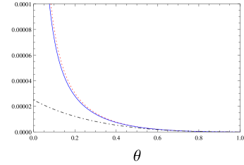
Figure 1: Work, scaled by $N$, as a function of $\theta$ for $a=0.01$. The dotted top curve is for optimal work $W_{o}$, middle solid curve is the estimate $\tilde{W}_{p}$, with the derived prior, and the lower dotdashed curve is the estimate $\tilde{W}_{u}$, with uniform prior. The three curves agree in the near equilibrium regime ($\theta\approx 1$).

Note that the above estimates for work are the same for both the observers, again due to symmetry in the work expression (17) w.r.t $T_{1}$ and $T_{2}$.

Fig. 1 illustrates the comparison for a given value of $a$. The agreement between different estimates in the near-equilibrium regime ($\theta\approx 1$), can be studied by expanding the work estimates about $\theta=1$:

$$\tilde{W}_{p}\approx\tilde{W}_{u}=\frac{Na^{2}}{16}(1-\theta)^{2}+\frac{3Na^{2}}{32}(1-\theta)^{3}+~{}O[1-\theta]^{4}.$$ (23)

These estimates of work agree with the optimal work upto third order of $(1-\theta)$. Fig. 2 shows the comparison of ${W}_{o}$, $\tilde{W}_{p}$ and $\tilde{W}_{u}$ for more general values of parameter $a$, when the constraint of entropy conservation can be treated numerically only. We observe the close agreement in the estimates for near-equilibrium. However, in general, the estimates from the derived prior are much better estimates of the optimal work than obtained from uniform prior, thus signifying the use of prior information in the assignment of the prior.

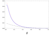
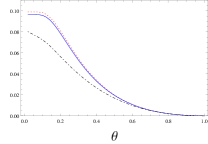
(a)	(b)
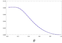
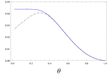
(c)	(d)

Figure 2: Work, scaled by $N$, as a function of $\theta$ for different $a$’s values; (a) $a$ = 0.2, (b) $a$ = 0.8 , (c) $a$ = 1.5, (d) $a$ = 2.4. The dotted curve is for $W_{o}$, solid curve is for $\tilde{W}_{p}$, and dotdashed curve is for $\tilde{W}_{u}$.

III.3 Efficiency

Efficiency is defined as the ratio $\eta=W/Q_{\rm h}$. So in order to estimate efficiency, we have to estimate the amount of heat exchanged with the hot reservoir, $Q_{\rm h}$. However, as pointed out in the previous subsection, owing to a complete ignorance about the association of temperature labels with their reservoirs, the quantity $Q_{\rm h}$ can be written in two ways. In terms of temperature $T_{2}$, we can either write

$$Q_{\rm h}(T_{2})=\frac{Na^{2}}{4}\left[\frac{1}{T_{2}}-1\right].$$ (24)

or, as

$$Q_{\rm h}^{\prime}(T_{2})=\frac{Na^{2}}{4}\left[{\sqrt{1+\frac{1}{\theta^{2}}-\frac{1}{{T_{2}}^{2}}}}-1\right].$$ (25)

Then the estimate for heat absorbed from the hot reservoir can be given by either $Q_{\rm h}(\overline{T}_{2})$ or $Q_{\rm h}^{\prime}(\overline{T}_{2})$.

It follows that the efficiency can be estimated in two ways: $\tilde{\eta}_{1}=\tilde{W}/{Q}_{\rm h}(\overline{T}_{2})$ or $\tilde{\eta}_{2}=\tilde{W}/{Q}_{\rm h}^{\prime}(\overline{T}_{2})$, where $\tilde{W}$ is given by Eq.(21). Explicitly, we obtain

$$\tilde{\eta}_{1}=\frac{\sqrt{3\theta^{2}-2\theta+3}-(1+\theta)}{1-\theta},$$ (26)

and

$$\tilde{\eta}_{2}=\frac{\sqrt{3\theta^{2}-2\theta+3}-(1+\theta)}{\sqrt{3\theta^{2}-2\theta+3}-2\theta}.$$ (27)

We now compare the above estimates with the efficiency at optimal work, which by using Eq. (19), is given as:

$${\eta}_{o}=2\left(\frac{\sqrt{2(1+\theta^{2})}-(1+\theta)}{\sqrt{\frac{1+\theta^{2}}{2}}-\theta}\right).$$ (28)

Fig. 3 shows these comparative plots. The estimates expanded near equilibrium are as follows:

$$\tilde{\eta}_{1} \approx \frac{\eta_{c}}{2}+\frac{{\eta_{c}}^{2}}{4}+\frac{1}{16}{\eta_{c}}^{3}+O[{\eta_{c}}^{4}],$$ (29)

$$\tilde{\eta}_{2} \approx \frac{\eta_{c}}{2}-\frac{1}{16}{\eta_{c}}^{3}+O[{\eta_{c}}^{4}],$$ (30)

whereas near equilibrium, the efficiency at optimal work, behaves as:

$${\eta}_{o} \approx \frac{\eta_{c}}{2}+\frac{{\eta_{c}}^{2}}{8}+O[{\eta_{c}}^{4}].$$ (31)

In this situation, we observe agreement with the optimal behavior only upto first order.

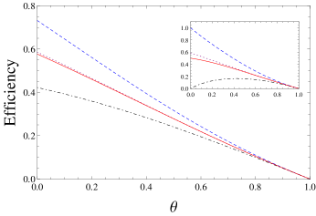
Figure 3: Efficiency vs. $\theta$. The solid curve is the mean estimate $\tilde{\eta}$, closely following the dotted curve which is for optimal value $\eta_{o}$. The top and the bottom curves are $\tilde{\eta}_{1}$ and $\tilde{\eta}_{2}$. The inset shows the corresponding quantities with the use of uniform prior.

On the other hand, if we define a mean estimate for efficiency as $\tilde{\eta}=(\tilde{\eta}_{1}+\tilde{\eta}_{2})/2$, then the agreement of this mean with the optimal behavior is upto third order. The use of a mean estimate can be justified as follows. We have two hypotheses, whether the heat extracted is given by Eq. (24) or (25). According to Laplace’s principle of insufficient reason Laplace1774 , when we do not have specific reason to prefer one hypothesis over another, then we should assign equal weights to the inferences following from each of these hypotheses. In our case, we have assumed complete ignorance about the labels attached with final temperatures and so each expression for $Q_{\rm h}$ above is equally valid. In this sense, it is reasonable that the most unbiased estimate be based on an equally-weighted mean of the different estimates.

It is to be noted that this property also emerges during the use of a uniform prior. Thus we can see analytically that in the near equilibrium case for small $a$ values, the uniform prior as well as the non-uniform prior both replicate the optimal properties of the work as well as efficiency to terms beyond linear response. However, as corroborated by the full numerical calculations for arbitrary $a$ and for general temperature differences (Figs. 2 and 3), it is apparent that the estimates with the non-uniform prior provide a quite good agreement with the optimal properties than the uniform prior.

IV Thermal Interaction

In this section, we study another well-known process in which two finite reservoirs interact thermally with each other, while conserving the total energy. A little amount of heat energy is quasi-statically removed from the hot reservoir and deposited in the same manner with the cold reservoir. The optimal process is the one which terminates at a common temperature. As is known, there is a net entropy production in the reservoirs. We consider a situation in which the final state after interaction is not specified, and so we have to estimate the final state. As in previous sections, we need to derive the prior to quantify our uncertainty about the value of the final temperatures.

Now the prior $\pi(T)$ will be derived from the information that the transfer of an infinitesimal energy from the hot to the cold reservoir, does not change the total energy:

$$dU_{1}+dU_{2}=0,$$ (32)

which can be written as:

$$\frac{\partial U_{1}}{\partial T_{1}}dT_{1}+\frac{\partial U_{2}}{\partial T_{2}}dT_{2} = 0.$$ (33)

This yields $|{dT_{1}}/dT_{2}|=C_{2}(T_{2})/C_{1}(T_{1})$. Again similar to Eq. (6), we have $|{dT_{1}}/dT_{2}|=\pi(T_{2})/\pi(T_{1})$, Identifying these two conditions and using separation of variables, we obtain the prior for each of final temperatures, in the form

$$\pi(T_{i})=\frac{C_{i}(T_{i})}{\int_{\theta}^{1}C_{i}(T_{i})dT_{i}}.$$ (34)

The estimation of various quantities follows the similar procedure as highlighted in Section III. Here also, the constraint equation of energy conservation: $U_{1}+U_{2}=U_{+}+U_{-}$, cannot be solved to yield an explicit relation between $T_{1}$ and $T_{2}$. We can perform analytical calculations only for the high temperatures case. The main quantity of interest will be the net entropy production.

IV.1 High-temperature limit

The explicit relation between $T_{1}$ and $T_{2}$ is obtained by using Eq. (12) and total energy conservation of the reservoirs. This yields

$$T_{1}=\left(1+\frac{1}{\theta}-\frac{1}{T_{2}}\right)^{-1}.$$ (35)

For the optimal process, $T_{1}=T_{2}=T_{c}$, where $T_{c}=2\theta/(1+\theta)$. The expected value of one of the temperatures ($T_{i}$) over the informative prior (Eq. (34)), is calculated as:

$$\overline{T}_{i}=\frac{\theta\ln({1/\theta})}{(1-\theta)}.$$ (36)

The entropy produced $\bigtriangleup S=S_{1}+S_{2}-S_{+}-S_{-}$, can be written using Eq. (13) as:

$$\bigtriangleup S=\frac{Na^{2}}{8}\left(1+\frac{1}{\theta^{2}}-\frac{1}{{T_{1}}^{2}}-\frac{1}{{T_{2}}^{2}}\right),$$ (37)

which can be expressed as function of one variable, using Eq. (35). Then the estimate for entropy production in the high-temperature limit, is given by replacing $T_{i}$ with $\overline{T_{i}}$. The estimation was done with informative as well as uniform prior and compared with the optimal behavior. Fig. 4 shows the comparison in the limit $a/T\ll 1$.

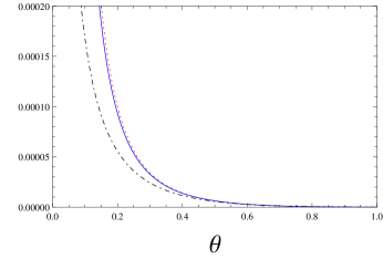
Figure 4: Entropy production, scaled by $N$, as a function of $\theta$ for $a=0.01$ in thermal contact process. The top, dotted curve is the optimal entropy production, the middle, solid curve is the estimate using informative prior, and lower, dotdashed curve is from the use of uniform prior.

When we expand the estimates for entropy production in near-equilibrium regime, we get:

$${\bigtriangleup{S}}_{p}\approx{\bigtriangleup{S}}_{u} = \frac{Na^{2}}{16}(1-\theta)^{2}+\frac{Na^{2}}{8}(1-\theta)^{3}+O[1-\theta]^{4}.$$

These estimates show agreement with the optimal entropy production upto third order, as in the case of estimated work in Section III.1.

Finally, for general $a$ values, the numerical calculations show that the estimated entropy production with the derived prior shows a good agreement with the optimal entropy production, along similar lines as for estimates of extracted work.

V Discussion

In this section, we try to gain an insight into the form of prior. First we note that the prior for final temperature in the entropy conserving process, Eq. (6), can be reexpressed as:

$$P(T)dT=\frac{dS}{(S_{+}-S_{-})}.$$ (39)

Thus the derived prior is equivalent to a uniform prior in terms of the entropy, defined over the interval $[S_{-},S_{+}]$. Similarly, the prior for the energy conserving process, Eq. (34), implies a uniform prior over the energy of a reservoir: $\pi(T)dT=dU/(U_{+}-U_{-})$. Thus our particular choice of prior for temperature, implies a uniform prior density for the quantity being conserved in the process.

Secondly, the proposed prior lends a specific meaning to the final common temperature ($T_{c}$). For the optimal entropy conserving process, the change in entropy of a reservoir is given by: $S_{+}-S_{c}=S_{c}-S_{-}$. This can be written in integral form as:

$$\int_{S_{c}}^{S_{+}}dS=\int_{S_{-}}^{S_{c}}dS.$$ (40)

As the prior density is uniform in terms of entropy, so we can write

$$\int_{S_{c}}^{S_{+}}p(S)dS=\int_{S_{-}}^{S_{c}}p(S)dS,$$ (41)

where $p(S)=1/(S_{+}-S_{-})$. Thus our choice of prior implies that we are assigning equal probability (one-half each) that entropy $S$ of a reservoir may lie in the interval $[S_{-},S_{c}]$, or in the interval $[S_{c},S_{+}]$. A similar statement can be made in terms of $T_{c}$. Thus $T_{c}$ is the median of prior $P(T)$, on either side of which we expect equal chances that the final temperature may lie.

The whole analysis can also be looked at in terms of macrostates. Consider the basic question in equilibrium thermodynamics Callen1985 . Given that entropy is conserved for a bipartite system whose total energy is allowed to vary, what is the most likely state of the system? The answer is given as the equilibrium state which has minimum total energy for the given value of the total entropy. (In terms of work, it translates into an extraction of maximum work.) The agreement of our estimates with the optimal work and the corresponding efficiency which was found in Section IV, shows that we are able to estimate the equilibrium state consistent with the constraints, without explicitly doing an optimization.

Finally, let us analyse the expected value of temperature as defined by $\overline{T}=\int TP(T)\,dT$. For the entropy conserving process, by using Eq. (6), the estimate for temperature has the general form:

$$\overline{T} = \frac{1}{N}\int_{T_{-}}^{T_{+}}{C(T)}\;dT$$ (42)

$$= \frac{1}{N}\int_{U_{-}}^{U_{+}}\!dU$$

$$= \frac{(U_{+}-U_{-})}{(S_{+}-S_{-})},$$

where $N=\int C/T\;dT$. This suggests that $\overline{T}$ is the estimate for the derivative of the function $U(S)$ whose values at two points, $U_{+}(S_{+})$ and $U_{-}(S_{-})$, have been given. We note that the above intuitive meaning arises naturally within the energy representation Callen1985 . Similarly, if we consider pure thermal interaction, the prior is given as: $\pi(T)dT=CdT/\int CdT$. While there is no simple interpretation for the expected value of $T$ in this case, however the expected value of the inverse temperature $\beta=1/T$, is given simply as

$$\overline{\beta}=\frac{(S_{+}-S_{-})}{(U_{+}-U_{-})}.$$ (43)

So here, $\overline{\beta}$ can be regarded as an estimate for the derivative of the function $S(U)$, when its values at two points, $S_{+}(U_{+})$ and $S_{-}(U_{-})$, have been given. This is also consistent with the fact that in the entropy represntation, $\beta$ is the derivative of the function $S(U)$.

Concluding, we have extended the basic approach suggested in PRD2013 , to quantify uncertainty as subjective probability, in constrained thermodynamic processes. In this paper, we considered entropy conserving as well as energy conserving processes. We argued for and proposed a general prior while incorporating the prior information about the process. Depending on the kind of process, this general form is applied to the case of two spin-1/2 systems as heat reservoirs, to estimate the maximum extracted work and the corresponding efficiency or the net entropy production. The agreement with optimal values of these quantities are shown in high temperatures limit, as well as by numeric calculations. Finally, in order to elucidate the meaning of the prior, we found certain points of consistency of our approach with the standard axiomatic thermodynamic framework. In our opinion, our approach seems applicable to quantify uncertainty in a subjective sense, for other constrained optimization problems. Further, some interesting future problems may be cited as: generalization to multipartite systems and the use of non-identical reservoirs.

VI Acknowledgements

RSJ acknowledges financial support from the Department of Science and Technology, India under the research project No. SR/S2/CMP-0047/2010(G). PA is thankful to University Grants Commission, India for Research Fellowship.

References

- (1) J. Bernoulli, The Art of Conjecturing, together with Letter to a Friend on Sets in Court Tennis, translated by Edith Dudley Sylla, Johns Hopkins University Press, (Baltimore, 2006).
- (2) P.S. Laplace, “Memoir on the Probabilities of the Causes of Events”, translated by S.M. Stigler, Stat. Sc. 1, 364-378 (1986).
- (3) T. Bayes, “An Essay towards solving a Problem in the Doctrine of Chances”, contributed by Mr. Price, Phil. Trans. Roy. Soc. 53, 370-418 (1763). Reprinted in Biometrika, 45, 296–315 (1958).
- (4) H. Jeffreys, Theory of Probability, Third edition, Clarendon Press, Oxford (1961).
- (5) E.T. Jaynes, IEEE Trans. on Systems Science and Cybernetics, SSC-4 227 (1968).
- (6) G. D’Agostini, Revista de la Real Academia de Ciencias 93 (1999), special issue on Bayesian Methods in the Sciences, edited by J.M. Bernardo.
- (7) S. James Press, Subjective and Objective Bayesian Statistics: Principles, Models and Applications, Second Edition, John Wiley and Sons, Inc. (2003).
- (8) For a review, see: R.E. Kass and L. Wasserman, J. Am. Stat. Assoc. 91, 1343 (1996).
- (9) J. Skilling, in Maximum Entropy and Bayesian Methods, edited by J. Skilling (Kluwer, Dordrecht, 1989), pp. 45-52.
- (10) C.C. Rodriguez, in Maximum Entropy and Bayesian Methods, edited by J. Skilling (Kluwer, Dordrecht, 1989), pp. 415-422.
- (11) A. Zellner, in Maximum Entropy and Bayesian Methods, edited by W.T. Grandy Jr. and L.H. Schick (Kluwer, Dordrecht, 1991).
- (12) A. Caticha and R. Preuss, Phys. Rev. E 70, 046127 (2004).
- (13) C.R. Rao, in Differential Geometry in Statistical Inference, 10, Institute of Mathematical Statistics Lecture Notes-Monograph Series, Institute of Mathematical Statistics, Hayward, California, Chap. 5, pp. 217-240.
- (14) For simplicity, we denote both the uncertain variable as well as its value by a capital symbol.
- (15) P. Aneja and R.S. Johal, Proceedings of Sigma-Phi International Conference on Statistical Physics-2011, Cent. Eur. J. Phys. 10 (3) 708 (2012).
- (16) P. Aneja and R. S. Johal, J. Phys. A: Math. Theor. 46, 365002 (2013).
- (17) R. Baeirlein, Atoms and Information Theory, W.H. Freeman and Company, San Francisco (1971).
- (18) As an alternative, we may choose to ignore the mutual dependence of parameters and while assigning the prior. Then a plausible prior is the uniform density, .
- (19) For a justification of this method by substitution, see PRD2013 .
- (20) For a further discussion on the so-called label uncertainty, see: R.S. Johal, R. Rai and G. Mahler, Bounds on Thermal Efficiency from Inference, arXiv:1305.6278v1, submitted for publication (2014).
- (21) H. B. Callen, Thermodynamics and an Introduction to Thermostatistics, 2nd ed.(John Wiley, New York, 1985).