Measuring the degree of unitarity for any quantum process
Abstract
Quantum processes can be divided into two categories: unitary and non-unitary ones. For a given quantum process, we can define a degree of the unitarity (DU) of this process to be the fidelity between it and its closest unitary one. The DU, as an intrinsic property of a given quantum process, is able to quantify the distance between the process and the group of unitary ones, and is closely related to the noise of this quantum process. We derive analytical results of DU for qubit unital channels, and obtain the lower and upper bounds in general. The lower bound is tight for most of quantum processes, and is particularly tight when the corresponding DU is sufficiently large. The upper bound is found to be an indicator for the tightness of the lower bound. Moreover, we study the distribution of DU in random quantum processes with different environments. In particular, The relationship between the DU of any quantum process and the non-markovian behavior of it is also addressed.
pacs:
03.67.-a, 03.65.YzI Introduction
Quantum computation is of great interest in recent years for its great speed up for solving some problemsShor1994 ; Grover1997 and its efficiency in simulating physical systemsFeynman1982 . Ideally, a quantum computer is a closed quantum system, and the evolution of the system is a unitary operation. However, as any quantum computer is inevitably interacted with the environment, the system is more or less open, and thus the system evolution becomes non-unitary. This is one of major difficulties for making a large scale quantum computer.
When a quantum system becomes open, the information about the initial state may be lost after the evolution of the system, and we cannot undo a quantum operation in general. This is discussed in quantum commutation, where quantum channel capacity is introduced to describe the information transfer ability of a quantum channel (see, e.g., Ref. Nielsen2000 ). Quantum channel capacity also illustrates the quantum channel noise. Notably, there are also other ways to study the noise of a quantum channel, such as using the addition of noise to change a quantum map into an entanglement-breaking map Pasquale2012 .
Since we can divide quantum operations into two categories: the unitary operations which are ideal, and the non-unitary ones which are most of the cases in real quantum systems, it is nature to ask to what extend a general quantum operation deviates from the group of unitary quantum operations, which appears to be fundamentally important. We here treat all of the unitary operations as a group because the information of a general quantum state can be perfectly preserved for all unitary operations.
To study the distance between a given quantum operation and the group of unitary operations, a common way is to find the closest unitary quantum operation for the given one, and use the distance between these two operations as the distance between the given quantum operation and the unitary operation group. The measure of the distance between two quantum processes has already been well studiedNielsen ; Nielsen2005 ; Grace2010 ; Zpuchala2011 , and we choose quantum process matrix fidelity in this paper. We define the fidelity between a given quantum process and its closest unitary one as the degree of unitarity(DU) of this given quantum process.
We think the study of the measure of the DU is important because of the following reasons. First of all, DU quantifies the difference between a realistic quantum operation and the ideal ones. It is an important intrinsic property for a quantum operation. Also, the DU of a quantum process is closely related to the noise of this process, the quantum capacity, and some other physical quantities such as the non-markovian behavior of a quantum process.
To obtain the DU of a given quantum process, a core problem we need to solve is to find the closest unitary operations of the given quantum process, since an analytical result for the measure of the distance between two quantum processes has already been available Nielsen ; Nielsen2005 ; Grace2010 ; Zpuchala2011 . However, finding an optimal unitary matrix is in general difficult because the optimization should be taken over all the unitary matrices. Remarkably, we here obtain analytical results for all qubit unital channels. Moreover, we also reveal the upper and lower bounds for the DU of a general quantum process. The lower bound is very tight and deviates from the true value slightly for most quantum processes, and it can be treated as a good approximation of the DU in most cases.
Our paper is organized as follows. In the next section (Sec. II), we give the definition of the DU of a quantum process and address its properties. In Sec. III, we give analytical results for qubit unital channels and some other special cases. In Sec. IV, we reveal the upper and lower bounds for the DU of a quantum process in general cases, and discuss the tightness of the bounds. In Sec. V, we study the probability distribution of DU of a quantum system interacting with environment of different dimensions. Finally, we present a brief summary and outlook in Sec. VI.
II Definition and properties
A quantum process can be expressed in Kraus operatorsKraus1983 ,
| (1) |
where the operators satisfy to insure this is a trace preserving map. The Kraus operator representation has clear physical meaning and every part of the summation can be treated as the evolution of the system when the environment is measured and a specific result is obtained. But since we need a group of matrices to represent a quantum process using Kraus operators, sometimes it is more convenient to use quantum process matrix to describe a quantum process which only need one matrix .
Suppose is an orthogonal basis set for the system, let , then the quantum process can be expressed as
| (2) |
where is called the quantum process matrix which contains all the information of the quantum process.
For a given quantum process and a unitary operation , how to measure the distance between them has been widely discussedNielsen ; Nielsen2005 ; Grace2010 ; Zpuchala2011 . One way is consider the difference of the out put states for and . As we want the distance between two processes to be independent of the initial state, a nature way is to average over all the initial states. If we choose fidelity to measure the difference of the output states, the distance between the processes can be measured by
| (3) |
Here is the initial state of the system. The integration is carried over the whole Hilbert space of the quantum state of the system, and the volume of the state is calculated according to Harr measure.
The average fidelity measure not only has clear physical meaning, but also has analytical expression.
In Ref.Nielsen , they give an analytical result in this formula:
| (4) |
where is the dimension of the system.
Another way to measure the distance is to measure the distance between the quantum process matrices directly. We also choose fidelity to measure the distance between process matrices. Then the fidelity between two processes is
| (5) |
where .
It turns out that the average fidelity measure of two quantum processes and the fidelity between two process matrices is related by the formula belowNielsen2005 :
| (6) |
Substituting it into Eq. (4), we can get that
| (7) |
We choose to measure the distance between the quantum process and the unitary evolution in this paper. The reasons for this will be stated later in this section. In the following, we denote as for simplicity.
Now we consider the main topic of this paper, the measure of the degree of unitarity(DU) for a given quantum process . As it is discussed in Sec. I, we choose the nearest unitary operation for the given quantum process and use to measure the distance between and . We define as the DU for .
This definition can be treated as the geometry measure of the DU, and the geometry measure is also used in other cases such as quantum discordLuoshunlun2010 .
According to the definition and Eq. (7), the DU of a quantum process is,
| (8) |
Generally, it is hard to get analytical result for the above expression as the optimization is over all the unitary matrices. Luckily in this problem for some special cases we can get clean result. We will discuss this in details in the next section.
Here we focus on the properties of DU to illustrate that this is indeed a reasonable definition and measures the similarity between a general quantum process and unitary ones.
First, the of should be a property of the process and should not be depended on the choice of Kraus operators . This property is assured by that the average fidelity is independent of the choice of the Kraus operatorsNielsen .
Also, the DU of should not be smaller than the DU , which means that the quantum process cannot become more unitary by subsequent processes. This is also guaranteed by the properties of average fidelityNielsen2000 . This property also make the DU as an indicator for non-markovian behavior of a quantum processBreuer2009 . It can be deduced that if DU increases during a quantum evolution, then this quantum evolution is non-markovian. However, the converse is not true.
Next we consider the extreme values of the DU of . When is unitary, the DU should reach its maximum. This can be easily confirmed because in this case the nearest unitary operation is itself and one can get that DU of this unitary process is 1. For the minimum of DU, intuitively, one can choose the quantum process(or quantum channel) to be a maximal depolarizing channel, which maps all the initial states into the maximum mixed state. In this case, one can choose arbitrary unitary operation as the nearest one, and the DU of this process is equal to .
Finally we discuss the difference between the DU of and , where is a unitary operation acting on an additional quantum system. One can verify that
| (9) |
which means that the DU of a given quantum process will not change by adding an unitary operation imposed on an ancillary quantum systems. Also one can verify that if we choose the average fidelity as the measure for two quantum processes, although the nearest unitary operation will not change, the above property will not be satisfied. This is the reason that we choose the process matrix fidelity measure.
One can also refer to Table 1 to get a clearer picture of DU, where the DU of some important qubit channel is listed. Table 1 can be get using the method provided in the next section.
III Analytical result for some special cases
To get the DU of a quantum process , we need to find the nearest from the group of unitary matrices. This is in general difficult. However, if the quantum process satisfies some properties, we can get analytical result.
We introduce the inner product in the operator space, and denote the inner product between two operators and as :
| (10) |
Then according to Eq. (8), the DU of the quantum process can be expressed as
| (11) |
So the DU of a quantum process is the sum of the square of the projections of the nearest on each Kraus operator. If each Kraus operator is a unitary operation multiplied by a constant, and they are orthogonal with each other, then the optimization process can be greatly simplified.
Theorem 1:
For a quantum process , if for all s and for , then
| (12) |
where is the coeficient with the max norm.
Proof:
Expand into a set of orthogonal basis in the operator space with operations . Then any unitary operation can be expressed as a linear combination of ,
| (13) |
where .
Then
| (14) | |||||
Suppose is the coefficient with the biggest norm. As , one can see that the above expression reaches its maximum when .
In this case, according to the expression of the DU of a quantum process in Eq. (8),
| (15) | |||||
This completes the proof.
Of course, the situation in Theorem 1 is a very special case, it requires all all the Kraus operators to be proportional to unitary operations and are orthogonal to each other at the same time. But one can notice that the representation of a quantum process using Kraus operators has its freedom and it turns out that every quantum process can be represented in orthogonal Kraus operatorsNielsen2000 .
Suppose a quantum process , let be the correlation matrix with . One can note that is a Hermitian matrix. We can diagonolize with unitary matrix
| (16) |
It can be proved that the rank of is at most, where is the dimension of the system.
Let
| (17) |
One can show that is equivalent with and
| (18) |
Further more, for a qubit channel, if the original Kraus operators s are proportional to unitary operations, then after diagonaliztion, the operators are still unitary operations. This theorem can be found in Ref.Bengtsson2006 . Here we give a different proof using the notations in this paper.
Proof:
Suppose the Kraus operators are , where , .
Follow the diagonalization process stated above, we can get the Kraus operators after diagonalization . Then
| (19) |
One can note that if is replaced by with , the quantum process will be the same as before. So we can treat all the s as SU(2) matrices. For a SU(2) matrix, one can represent it as
| (20) |
One can verify that is a real, and
| (21) |
Also one can notice that is an orthogonal matrix in this case, so is real too. On the r.h.s. of Eq. (19), if , is proportional to . If , as is real and is proportional to , is also proportional to . So we can get
| (22) |
where is a complex number. This condition implies that is proportional to a unitary operation.
Combined with Theorem 1 together, we can get that if a qubit channel is a convex combination of unitary channels, we can get analytical result for the DU of this channel.
For qubit channels, it can be shown that every unital channel is a convex combination of unitary channels, where a unital channel is a channel that maps into . This is related to Birkhoff conjecture, which is only true for Landau1993 . Since we can get analytical result for convex combination of unitary channels, we can get analytical result of the DU for all qubit unital channels.
Convex combination of unitary channels are of great interest as they are the only channels that can be perfectly inverted by monitoring the environmentGregoratti2003 . The calculation of DU for these channels offers a new perspective for the information and the noise of these channels.
Now we list the analytical result of DU in Table 1 for some important qubit channels, including depolarizing channel, bit flip channel, phase flip channel, and amplitude damping channel. We can see that the DU of these quantum channel is between and 1, as it is shown in Sec. II. For depolarizing channel, bit flip channel and phase flip channel, the nearest unitary operation changes when the parameter of the channel changes. For amplitude damping channel, the nearest unitary operation is always the identity operation.
| Channel | Kraus Operators | DU of this channel |
|---|---|---|
| depolarizing channel | , ,, | Max{} |
| bit flip channel | , | Max{} |
| phase flip channel | , | Max{} |
| amplitude damping channel | , |
IV Lower bound and upper bound for du in general cases
In general cases, it is hard to get analytical result for the DU of a quantum process. We try to get the lower bound and upper bound for DU in this section.
To get the lower bound, we try to find a unitary operation that is very close to the quantum process, although it may not be the closest. As it is hard to find the closest for all these Kraus operators, we try to find the closest for one of them.
One option is to find the nearest for the Kraus operator with the largest norm after diagonalization. Suppose the Kraus operators of after diagonalization are , and the norm of , , is the largest among all the s. Then the closest unitary matrix for , which is the unitary matrix that maximize , can be found though polar decomposition.
Suppose the polar decomposition of is
| (23) |
Then
| (24) | |||||
where the equality is obtained when . One can note that is the nearest unitary matrix for .
We choose as the approximation of the nearest unitary operation for , and calculate the DU of this quantum process. Then we get the lower bound for DU of ,
| (25) |
Also as s are orthogonal with each other, the contribution of is relatively small if is not 1, i.e., if is not the Kraus operator with the largest norm. So we can also choose as a simplified lower bound, which equals , where s are the singular value of . This lower bound equals the largest visibility the interference between and unitary channels, and it can be got experimentallyOi2003 .
We can get the lower bound in another way. We choose the Kraus operator that may contribute most to as the major part, of which the value is the maximum. One can note that chosen Kraus operator has the largest value of . Note that previously we choose the one with the largest value of . This two standards may make different when the derivation of s is large. We denote the major Kraus operator by this new standard as , and the nearest unitary operation of as , then the new low bound for is
| (26) |
Now we consider the upper bound of the DU of a quantum process. We assume the nearest of is the nearest unitary operation of all the Kraus operator s, which means that there is a unitary operation that makes reaches its largest value for all s. Apparently, this is not possible for most cases. But it give a upper bound for the DU of this quantum process.
According to Eq. (24), the largest value of is . So we can get a upper bound for ,
| (27) |
We can show that the upper bound of is less or equal than 1. As
| (28) | |||||
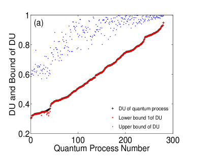
Now we consider the tightness of the lower bound and upper bound. We denote the lower bound in Eq. (25) as lower bound 1, and the one in Eq. (26) as lower bound 2.
We randomly choose a quantum process and calculate the DU of the quantum process, two lower bounds of the DU, and the upper bound of DU. Also, in order to study the bound behavior as a function of the DU, we choose approximately equal amount of quantum processes for each interval of the DU of quantum processes. As shown in Fig. 1(a), the lower bound of DU(red stars) is a good approximation of DU(black cross) in almost all the cases. Particularly,when DU is larger than 0.4, the lower bound of DU(red stars)is almost the same as DU. When the DU of a quantum process is very small, the lower bound may differs from the true value for about 10%.
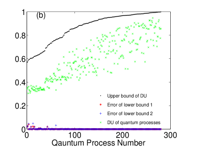
On the other hand, the upper bound of DU is quite loose. But it can be shown that the upper bound may be a indicator of the behavior of the lower bound. As shown in Fig. 1(b), the difference of two lower bounds of DU from the true value are almost zero when the upper bound of DU is bigger than 0.8. When the upper bound of is small, the error of the lower bound may be large.
V The probability distribution of the du of a qubit system with different environment
In this section, we consider the probability distribution of the DU of a random quantum process for a quantum system. This distribution can give us some information for the DU of a random quantum process before we really know it. It also gives the expected value of DU of the process of a quantum system. One can note that the distribution of DU depends on the dimension of the system and the environment. It is also related to how the system and the environment interacts with each other.
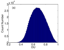
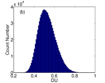
Here we study a qubit system. Suppose the qubit is fully interacting with an environment with an dimension of , and the evolution of the total system composed by the qubit and the environment is a random unitary operation with the dimension of . In this case, we study the probability distribution of DU of the operations imposed on the qubit system.
For simplicity, we only consider the cases when . We generate a random unitary operation for the total system according to the Harr measure, and calculate the DU for the corresponding quantum operations imposed on the principle qubit system. As it is already tested in Sec. IV that the lower bound of DU is very tight, we treated the lower bound of DU as DU in this calculation. As shown in Fig. 2, when the dimension of the system become bigger, the expected value for the DU is decreased. This means that the system is expected to be more open and the evolution of the system is expect to be more non-unitary.
VI Summary and outlook
In conclusion, we have investigated a key problem of the DU for any quantum process. We have introduced a definition of the DU of a quantum process and addressed its properties. The DU of a quantum process quantifies the distance between a given quantum process and the group of all unitary ones. It is closely related to the noise of the quantum process and is an indicator for non-markovian behavior of a quantum system. For qubit unital channels, we have obtained an analytical result of the DU. For general cases, we have derived the lower and upper bounds for the DU. We have presented two different lower bounds for the DU, both being quite tight in most cases. The upper bound of DU can be treated as an indicator for the tightness of DU. When the upper bound is low, the lower bound of DU may be less tight. We have also discussed the probability distribution of the DU of a qubit system interacting with different environments, and found that the DU tends to become smaller when the dimension of the environment become bigger.
The study of DU of a quantum process raises many related issues to be investigated in near future, such as the relationship between DU of a quantum process and the noise of a quantum process according to other measures, the DU’s evolution behavior for a real physical system, the DU for the quantum process in an open quantum system based quantum algorithmMizel2009 ; Long2011 and so on.
Acknowledgements.
We thank Y. Hu and Z. Y. Xue for helpful discussions. This work was supported by the RGC of Hong Kong under Grant No. HKU7058/11P.References
- (1) R. Feynman, Int. J. Theor. Phys. 21, 467 (1982).
- (2) P. W. Shor, in Proc. 35th Symposium on the Foundations of Computer Science, (IEEE Computer Society Press), 124 (1994).
- (3) L.K. Grover, Phys. Rev. Lett. 79, 325 (1997).
- (4) M. A. Nielsen and I. L. Chuang, Quantum Computation and Quantum Information (Cambridge University Press, Cambridge, 2000).
- (5) A. De Pasquale and V. Giovannetti, Phys. Rev. A 86, 052302 (2012).
- (6) A. Gilchrist, N. K. Langford and M.A. Nielsen, Phys. Rev. A 71, 062310(2005).
- (7) M. A. Nielsen, Phys. Lett. A 303, 249(2002).
- (8) M.D. Grace, J. Dominy, R. L Kosut et. al, New Journal of Physics 12, 015001(2010)
- (9) Z. Puchała, J. A. Miszczak, P. Gawron et al, Quantum Information Processing 10(1), 1-12(2011).
- (10) Karl Kraus, A. Bo¨hm, J. D. Dollard, and W. H. Wootters, States, Effects, and Operations Fundamental Notions of Quantum Theory: Lectures in Mathematical Physics at the University of Texas at Austin, Lecture Notes in Physics, Vol. 190 (Springer, Berlin, 1983).
- (11) S. Luo and S. Fu, Phys. Rev. A 82, 034302(2010).
- (12) H. P. Breuer, E. M. Laine, and J. Piilo, Phys. Rev. Lett. 103, 210401(2009).
- (13) I. Bengtsson and K. Zyczkowski, Geometry of Quantum States: an Intro- duction to Quantum Entanglement (Cambridge University Press, 2006)
- (14) L.J. Landau and R.F. Streater, Lin. Alg. Applic. 193, 107-127 (1993).
- (15) M. Gregoratti and R.F. Werner, J. Mod. Opt. 50, 915 (2003).
- (16) D. K. L. Oi Phys. Rev. Lett. 91, 067902(2003).
- (17) A. Mizel, Phys. Rev. Lett. 102,150501(2009).
- (18) G. L. Long, Int. J. Theor. Phys. 50(2011).