Abstract

There is an increasing interest in studying the neural interaction mechanisms behind patterns of cognitive brain activity. This paper proposes a new approach to infer such interaction mechanisms from electroencephalographic (EEG) data using a new estimator of directed information (DI) called logit shrinkage optimized directed information assessment (L-SODA). Unlike previous directed information measures applied to neural decoding, L-SODA uses shrinkage regularization on multinomial logistic regression to deal with the high dimensionality of multi-channel EEG signals and the small sizes of many real-world datasets. It is designed to make few a priori assumptions and can handle both non-linear and non-Gaussian flows among electrodes. Our L-SODA estimator of the DI is accompanied by robust statistical confidence intervals on the true DI that make it especially suitable for hypothesis testing on the information flow patterns. We evaluate our work in the context of two different problems where interaction localization is used to determine highly interactive areas for EEG signals spatially and temporally. First, by mapping the areas that have high DI into Brodmann area, we identify that the areas with high DI are associated with motor-related functions. We demonstrate that L-SODA provides better accuracy for neural decoding of EEG signals as compared to several state-of-the-art approaches on the Brain Computer Interface (BCI) EEG motor activity dataset. Second, the proposed L-SODA estimator is evaluated on the CHB-MIT Scalp EEG database. We demonstrate that compared to the state-of-the-art approaches, the proposed method provides better performance in detecting the epileptic seizure.

1 Introduction

An extensive body of research focuses on the goal of identifying and classifying brain activity using electroencephalographic (EEG) data. Central to these efforts is developing an understanding of how the brain processes information to achieve specific tasks. Previous work ([1][2][6][7][11][19][20][21][26]-[32]) has shown that certain regions in the human brain have strong interactions. As introduced by Granger [15][27], the relation between two signals may be expressed in terms of the linear predictability of one signal by the knowledge of the immediate past of the other signal. The original Granger causality measure was restricted to stationary Gaussian time series but later versions relaxed this stationary assumption. However, the representation and detection of the information flow within the brain remains a challenging problem due to assumptions of linearity and Gaussianity in measurable brain signals..

Directed information (DI) provides a measure of information that is suitable for non-linear and non-Gaussian dependencies between different EEG signal sources. The DI was first proposed by Massey in 1990 as an extension of Shannon’s mutual information (MI) [16]. Different from MI, DI is an asymmetric function of the time-aggregated feature densities extracted from pairs of measurement sites [10]. In [26], Quinn et al. utilized unregularized DI to capture the non-linear and non-Guassian dependency structure of spike train recordings, where they estimated the DI with point process generalized linear models. In this case, parameter and model selection was performed using maximum likelihood estimates and minimum description length. However, while the use of directed information in this manner has been demonstrated to be superior to Granger’s measure and MI, due to the high dimensionality of the features and small sample size intrinsic to EEG signals, a direct implementation of an empirical DI estimator suffers from severe overfitting errors. In this paper, we introduce an improved estimate of DI, called logit shrinkage optimized directed information assessment (L-SODA). L-SODA is conceptually simple, is of low implementation complexity, and is mean-square optimal over the class of regularized directed information estimators. The main difference between our work and [26] lies in the fact that the proposed L-SODA approach to DI estimation controls overfitting errors using shrinkage regularization applied to a reduced set of the features of EEG signals. This work builds upon our previous efforts [37] on shrinkage optimized directed information assessment (SODA), and seeks to explicitly address the curse of dimensionality by applying shrinkage methods on multinomial logistic regression [41] to estimate likelihood functions required for evaluating the DI. Our experiments demonstrate that L-SODA’s performance is superior to state-of-the-art methods for neural interaction detection and classification.

There is an extensive literature related to EEG signal interaction detection and classification. The authors of [3] used MI to classify EEG data. Maximum mutual information is applied to feature selection for EEG signal classification [4]. In [2][31], a directed transfer function (DTF) with a linear autoregressive model has been employed to fit the data and interaction is deduced and characterized. In [23], Hesse et al. presented an adaptive estimation of Granger causality. Simulations demonstrate the usefulness of the time-variant Granger causality for detecting dynamic causal relations. In [32], Lotte et al. reviewed classification algorithms used to design Brain Computer Interface (BCI) systems based on EEG. In [27], Supp et al. identified the directionality of oscillatory brain interactions in source space during human object recognition and suggested that familiar, but not unfamiliar, objects engage widespread reciprocal information flow. In [28], Hinrichs et al. analyzed the timing and direction of information flow between striate (S) and extrastriate (ES) cortex by applying a generalized mutual information measure during a visual spatial attention task. In [29], Babiloni et al. presented advanced methods for the estimation of cortical connectivity from combined high-resolution EEG and functional magnetic resonance imaging (fMRI) data.

Unlike these previous efforts, L-SODA implements estimates of the conditional distributions of the features over each temporal segment given the features in previous segments. This is effectively a Markov model if a window of fixed width is used. Our L-SODA approach is completely data-driven. It relies solely on a non-parametric regularized estimate of the conditional feature probability distribution. To estimate these high dimensional conditional feature distributions, L-SODA implements a novel James-Stein shrinkage regularization method ensuring minimum mean-squared error (MSE) over the family of shrinkage estimators of DI. Such a shrinkage approach was adopted by Hauser and Strimmer [5] for entropy estimation, but without logistic models. The L-SODA approach to estimating DI used shrinkage regularization that minimizes estimator mean square error and provides asymptotic expressions for estimator bias, variance in addition to a central limit theorem (CLT). Here we apply L-SODA to obtain an empirical directed graph of interactions between EEG electrodes, using the CLT to specify p-values for testing the statistical significance of detected interactions via simulation and to control the false discovery rate on the putative edge discoveries in the graph.

To evaluate our work, we use two approaches. The first utilizes ground truth neural functional area locations (Brodmann areas) for validation of our localization results. The Brodmann areas were originally defined and numbered by Korbinian Brodmann based on the cytoarchitecture organization of neurons he observed in the cerebral cortex [43]. When applied to a brain computer interface (BCI) motor activity dataset, we show that the directed information graph discovered by L-SODA is consistent with activation of the known Brodmann areas of the brain associated with motor functions. Our second evaluation approach assesses the utility of the interactions discovered by L-SODA to improve a neural classification task. Specifically, for the CHB-MIT Scalp EEG dataset, we show that L-SODA has better ability to detect epileptic seizure onset.

For both these cases, L-SODA exhibits performance advantages over the unregularized DI estimation of Quinn et al [26]. Since L-SODA is specifically designed for low sample sizes, L-SODA can be viewed as an optimized shrinkage regularized estimator of directed information. Compared to other forms of regularization such as sparse representation with l1 regularization [41], the error of the logit shrinkage regularization approach can be analyzed and optimized in the mean square sense. The shrinkage regularization of L-SODA has significant performance gains in the low sample size regime, a regime that is typical for temporally windowed BCI data. Moreover, as described in [32], the features in BCI and CHB-MIT Scalp EEG databases are non-stationary since EEG signals may vary rapidly. We demonstrate by experiment that the proposed L-SODA algorithm is not only able to control false positive rate more accurately, but also has lower false negative rate in detecting significant information flow at given false positives level.

1.1 Summary of the main contribution

In this paper, we:

1. Propose a new approach (L-SODA) to infer neural interaction mechanisms from EEG signals using a novel estimator of DI with logit shrinkage optimized DI assessment.

2. Derive a central limit theorem for this novel estimator that can be used to assess statistical significance for interaction detection.

3. Illustrate that L-SODA can find interactions between anatomical regions of the brain that are plausible in the context of mapping to Brodmann functional areas [25] for different tasks.

We further demonstrate the superiority of this approach over existing methods for DI estimation using the BCI project dataset and the CHB-MIT Scalp EEG database:

1. In terms of sensitivity, as compared to unregularized DI, Granger’s measure and coherence measure, L-SODA is capable of detecting new interactions among EEG signal sources and has at least 5% better localization accuracy. The localization results are verified using neural pathway locations of motor activities and are not discovered by existing approaches when subjected to the same false discovery rate.

2. In terms of specificity, as compared to previous results based on unregularized DI estimation [26], L-SODA is better able to control false positive rate (type I error) while maintaining high interaction detection accuracy.

3. L-SODA improves classification accuracy by 6% relative to the performance of Hidden Markov Models (HMMs), mutual information (MI), Granger’s measure, coherence measure and unregularized DI estimation.

4. We demonstrate that compared to unregularized DI estimation [26], L-SODA has an 8% lower false negative rate (type II error) in detecting information flow at given level of false positives.

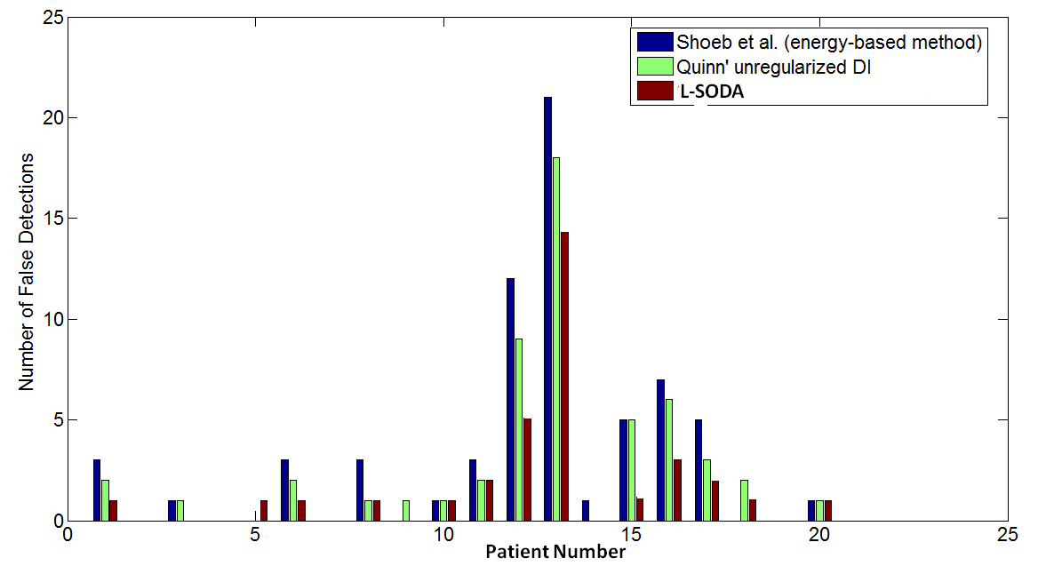
5. Moreover, by applying L-SODA with shrinkage logistic regression, we reduce the number of false positives for seizure detection by 3% compared to energy-based method and unregularized DI.

The rest of the paper is organized as follows: In Section 2, we present the statistical framework of L-SODA. In Section 3, we subsequently propose the L-SODA-based interaction detection algorithm. In Section 4, we evaluate the proposed algorithm and compare its performance with the state-of-the-art approaches. We conclude with a brief summary in Section 5.

2 L-SODA Framework for EEG

The SODA framework for directed information estimation was introduced in [37] for audio-video indexing. SODA is not scalable to high dimensional feature space since it requires discretization over the feature space in order to apply the multinomial model of [37]. To overcome this problem, here we augment this approach with the use of logit shrinkage (i.e., L-SODA) for use within the high dimensional EEG context.

The EEG is an aggregate measure of neurological activity within the brain. Consider two EEG electrodes $E_{x}$ and $E_{y}$ placed at positions $x$ and $y$ with $M_{x}$ and $M_{y}$ time points respectively. We denote by $X_{m}$ and $Y_{m}$ the temporal feature variables extracted at time $m$ for $E_{x}$ and $E_{y}$, and define $X^{(m)}=\{X_{k}\}_{k=1}^{m}$ and $Y^{(m)}=\{Y_{k}\}_{k=1}^{m}$. The mutual information (MI) between $E_{x}$ and $E_{y}$ is given by ${\mathrm{MI}}(E_{x};E_{y})=\textbf{E}\left[\ln\frac{\textbf{f}(\textbf{X}^{(M_{x})},\textbf{Y}^{(M_{y})})}{\textbf{f}(\textbf{X}^{(M_{x})})\textbf{f}(\textbf{Y}^{(M_{y})})}\right],$ where $f(X^{(M_{x})},Y^{(M_{y})})$ is a joint distribution and $\textbf{f}(X^{(M_{x})})$ and $\textbf{f}(Y^{(M_{y})})$ are marginal distributions. The DI from electrode $E_{x}$ to electrode $E_{y}$ is a non-symmetric generalization of the MI defined as

$${\mathrm{DI}}(E_{x}\Rightarrow E_{y}) = \sum_{m=1}^{M}I(X^{(m)};Y_{m}|Y^{(m-1)})~{},$$ (1)

where $M=\min\{M_{x},M_{y}\}$, $I(X^{(m)};Y_{m}|Y^{(m-1)})$=$\textbf{E}[\ln\frac{\textbf{f}(X^{(m)};Y_{m}|Y^{(m-1)})}{\textbf{f}(X^{(m)})\textbf{f}(Y_{m}|Y^{(m-1)})}]$ is the conditional MI between $X^{(m)}$ and $Y_{m}$ given the past $Y^{(m-1)}$. An equivalent representation of DI is in terms of the conditional entropies

$$H(X^{(m)}|Y^{(m-1)})=\textbf{E}[\ln\textbf{f}(X^{(m)}|Y^{(m-1)})],H(X^{(m)}|Y^{(m)})=\textbf{E}[\ln\textbf{f}(X^{(m)}|Y^{(m)})]$$

$${\mathrm{DI}}(E_{x}\Rightarrow E_{y})=\sum_{m=1}^{M}\left(H(X^{(m)}|Y^{(m-1)})\right)-\sum_{m=1}^{M}\left(H(X^{(m)}|Y^{(m)})]\right),$$ (2)

which gives the intuition that the DI is the cumulative reduction in uncertainty of time sample $Y_{m}$ when the past time samples $Y^{(m-1)}$ of $E_{y}$ are supplemented by information about the past and present segments $X^{(m)}$ of $E_{x}$. In the case that the feature sequences $X^{(M)}$ and $Y^{(M)}$ are jointly Gaussian, it is easily shown that the DI reduces to a monotonic function of Granger’s linear causality measure.

2.1 Previous SODA approach

SODA quantizes the feature variables to $p$ levels denoted as $\{z_{1},\ldots,z_{p^{m}}\}$. If the feature realizations are i.i.d. then $Z$ is multinomial distributed with probability mass function

$$P_{\theta}(Z_{1}=n_{1},\ldots,Z_{p^{m}}=n_{p^{m}})=\frac{n!}{\prod_{k=1}^{p^{m}}n_{k}!}\prod_{k=1}^{p^{m}}\theta_{k}^{n_{k}},$$

where $\theta=E[Z]/n=[\theta_{1},\ldots,\theta_{p^{m}}]$ is a vector of class probabilities and $\sum_{k=1}^{p^{m}}n_{k}=n$, where $n$ is defined as the number of experimental trials, $\sum_{k=1}^{p^{m}}\theta_{k}=1$. Since the number of quantization cells $p^{m}$ is larger than the number of trials $n$, a brute force plug-in estimation approach, e.g., using maximum likelihood (ML) estimates in place of $\theta$, is prone to overfitting error. Specifically, given $n$ independent samples $\{W_{i}\}_{i=1}^{n}$ of the EEG feature vector $W=[X^{(M_{x})},Y^{(M_{y})}]$ the ML estimator of the $k$-th class probability $\theta_{k}$ is $\hat{\theta}_{k}=n^{-1}\sum_{i=1}^{n}I(W_{i}\in C_{k})$, $k=1,\ldots,p^{M_{x}+M_{y}}$ where $I$ here is the indicator function. In [37], SODA shrinkage regularization was applied to reduce overfitting error.

2.2 L-SODA extension

To address the problem of high dimensionality of quantized feature space, in this work we use multinomial logistic regression for approximation of the conditional distribution [41] which obviates the need to perform joint discretization of $X$ and $Y$. In multinomial logistic regression, the logits,

$$\log\frac{P(X=k|y)}{1+\sum_{x\neq k}P(X=x|y)}=y^{T}\beta_{k}~{},$$ (3)

where $x$ and $y$ are discrete and continuous variables and $\beta_{k}$ is determined by a goodness of fit criterion [41], are modeled as a linear function. Using multinomial logistic regression approximation (3), the conditional probabilities required for computation of (2) become,

$$P(X^{(m)}=k|Y^{(m-1)})=\frac{\exp([Y^{(m-1)}]^{T}\beta_{k}(m-1))}{\sum_{j=1}^{p^{(m-1)}}\exp([Y^{(m-1)}]^{T}\beta_{j}(m-1))}~{},P(X^{(m)}=k|Y^{(m)})=\frac{\exp([Y^{(m)}]^{T}\beta_{k}(m))}{\sum_{j=1}^{p^{m}}\exp([Y^{(m)}]^{T}\beta_{j}(m))}~{}.$$ (4)

As compared to SODA, where both of $X^{(m)}$ and $Y^{(m)}$ are discrete and there are ($|\mathcal{C}|^{M_{x}+M_{y}}$) of multinomial parameters $\theta_{k}$. Here, in the L-SODA logistic regression approach only $X^{(m)}$ is quantized. This results in a reduction of multinomial dimensions from $|\mathcal{C}|^{M_{x}+M_{y}}$ to $|\mathcal{C}|^{M_{x}}$, which is significant in EEG applications considered in this paper. The regression coefficients $\beta=[\beta_{1},\ldots,\beta_{p^{m}}]$ are determined by maximum likelihood, with $\beta_{k}(m)$ denoting the weight vector corresponding to class $k$ for $P(X^{(m)}|Y^{(m)})$. Thus, the estimated directed information with multinomial logistic regression is:

$$\widehat{DI}_{\beta}=\sum_{m=1}^{M}\left[\frac{\exp([Y^{(m-1)}]^{T}\hat{\beta}_{k}(m-1))}{\sum_{j=1}^{p^{m-1}}\exp([Y^{(m-1)}]^{T}\hat{\beta}_{j}(m-1))}\log\frac{\exp([Y^{(m-1)}]^{T}\hat{\beta}_{k}(m-1))}{\sum_{j=1}^{p^{m-1}}\exp([Y^{(m-1)}]^{T}\hat{\beta}_{j}(m-1))}\right]$$

$$-\left[\frac{\exp([Y^{(m)}]^{T}\hat{\beta}_{k}(m))}{\sum_{j=1}^{p^{m}}\exp([Y^{(m)}]^{T}\hat{\beta}_{j}(m))}\log\frac{\exp([Y^{(m)}]^{T}\hat{\beta}_{k}(m))}{\sum_{j=1}^{p^{m}}\exp([Y^{(m)}]^{T}\hat{\beta}_{j}(m))}\right]~{},$$ (5)

Since $n\ll p^{\max\{|\mathcal{C}|^{M_{x}}\}}$, we propose to use James-Stein shrinkage regularization to reduce the MSE of the DI estimator. The resultant shrinkage optimized DI estimator, $\widehat{DI}^{\lambda_{\circ}}(X^{M}\Longrightarrow Y^{M})$ shrinks the maximum likelihood estimator $\hat{\beta}_{k}^{ML}$ towards a target coefficient vector.

$$\hat{\beta}_{k}^{\lambda}=\lambda t_{k}+(1-\lambda)\hat{\beta}_{k}^{ML}~{},$$ (6)

It is customary in James-Stein shrinkage to select targets that are minimally informative, e.g. uniform density [5][37]. Correspondingly, we select $t_{k}$ so that $t_{k,l}=\sqrt{\frac{1}{Var(y_{l})}}$, namely, $t_{k,l}$ is inversely proportional to the standard deviation of $y_{l}$, where $k$ is the index of class and $t_{k,l}$ represents the $l$th element in the target coefficient vector $t_{k}$. The James-Stein plug-in estimator for directed information with logistic regression is:

$$\widehat{DI}^{\lambda}_{\beta}=\sum_{m=1}^{M}[\frac{\exp([Y^{(m-1)}]^{T}\hat{\beta}_{k}^{\lambda}(m-1))}{\sum_{j=1}^{p^{m-1}}\exp([Y^{(m-1)}]^{T}\hat{\beta}_{j}^{\lambda}(m-1))}\log\frac{\exp([Y^{(m-1)}]^{T}\hat{\beta}_{k}^{\lambda}(m-1))}{\sum_{j=1}^{p^{m-1}}\exp([Y^{(m-1)}]^{T}\hat{\beta}_{j}^{\lambda}(m-1))}$$

$$-\frac{\exp([Y^{(m)}]^{T}\hat{\beta}_{k}^{\lambda}(m))}{\sum_{k=1}^{p^{m}}\exp([Y^{(m)}]^{T}\hat{\beta}_{k}^{\lambda}(m))}\log\frac{\exp([Y^{(m)}]^{T}\hat{\beta}_{k}^{\lambda}(m))}{\sum_{j=1}^{p^{m}}\exp([Y^{(m)}]^{T}\hat{\beta}_{j}^{\lambda}(m))}]~{},$$ (7)

The corresponding plug-in estimator for DI is simply $\widehat{{\mathrm{DI}}}^{\lambda}_{\beta}={\mathrm{DI}}_{\hat{\beta}^{\lambda}}(E_{x}\rightarrow E_{y})$. We specify the optimal value of $\lambda$ that minimizes estimator MSE: $\lambda^{\circ}=\arg\min_{\lambda}E(\widehat{DI}^{\lambda}_{\beta}-DI)^{2}~{}$. The MSE can be decomposed into the square of bias and variance and the optimal value of $\lambda_{\beta}$ can be obtained by minimizing MSE over $\lambda_{\beta}$ using a gradient descent algorithm.

3 L-SODA-based Interaction Detection Algorithm

In [37], a local version of DI was introduced for temporal localization of interactions. This is an important step for studying physiological signals such as the EEG, due to issues related to time warping inherent in these data. Here we describe the L-SODA algorithm in the context of EEG. Once the DI optimal shrinkage parameter has been determined, the local DI is defined similarly to the DI except that, for a pair of EEG signals $X$ and $Y$, the signals are time shifted and windowed prior to DI computation. Specifically, let $\tau_{x}\in[0,M_{x}-T]$, $\tau_{y}\in[0,M_{y}-T]$ be the respective time shift parameters, where $T\ll\min\{M_{x},M_{y}\}$ is the sliding window width, and denote by $X_{\tau_{x}}^{M_{x}}$, $Y_{\tau_{y}}^{M_{y}}$ the time shifted sequences. Then the local DI, $\mathrm{DI}(X^{M_{x}}_{\tau_{x}}\rightarrow Y^{M_{y}}_{\tau_{y}})$, computed using (1), defines a surface over $\tau_{x},\tau_{y}$. We use the peaks of the local DI surface to detect and localize the interactions in the pair of EEG signals. We implement L-SODA for EEG interaction detection using the following procedure:

1. Temporal Alignment: Align the EEG signals temporally by segmenting the EEG signals according to local DI peak locations to capture the beginning and ending times.

2. Pairwise DI and p-value computation: After alignment, calculate the $K$ $\times$ $K$ matrices of SODA estimated DI’s and p-values $1-\Phi\left(\frac{\hat{D}_{ij}-\mu_{ij}}{\sigma_{ij}}\right)$ on these DI estimates here $K$ equals 19, the number of electrodes.

3. False Discovery Rate Control: Threshold the DI and $p$-value matrices to find interaction regions exhibiting large and statistically significant DI. The bootstrap is used to estimate the mean and variance in the p-value matrix. The construction of the interaction graph over the $K$ EEG electrodes is performed by testing the $K\times(K-1)$ hypotheses that there is a significant interaction (both directions) between pairs of electrodes. Since there are $K(K-1)$ different DI pairs, this is a multiple hypothesis testing problem and we control false discovery rates using the corrected Benjamini- Hochberg (BH) procedure [35]. It tolerates more false positives, and allows fewer false negatives. The corrected BH procedure is implemented as follows:

   • The p-values of the $M=K(K-1)$ edges $(1,2,\ldots,M)$ are ranked from lowest to highest, all satisfying the original significance cut-off $p=0.05$. The ranked p-values are designated as $p_{(1)}$, $p_{(2)}$, $\ldots$ , $p_{(M)}$.

   • For $j=1,2,\ldots,M$, the null hypothesis (no edge) $H_{j}$ is rejected at level $\alpha$ if $p_{(j)}\leq(j/m)/\left(\sum_{n=1}^{M}n^{-1}\right)\alpha$, where $\alpha$ is the chosen acceptable p-value.

   • All the edges with p-value$\leq p_{(j)}$ are retained in the final network.

4 Experimental Results

4.1 BCI Project Database

The L-SODA algorithm was applied to the public BCI dataset consisting of EEG signals associated with motor activity [17]. The EEG consists of random movements of the left and right hand recorded with eyes closed. The data consisted of multiple data matrices corresponding to multiple activities, where each column of a data matrix represented one electrode and there are a total of 19 electrodes. Each row of a data matrix presented the temporal sample of electrical potential from one electrode and there were a total of 3008 samples in each row. The motor activity lasted about 6 seconds. The sampling rate of the recording was 500Hz. The data in BCI project consisted of EEG signals. The subject executed 10 classes of movements where each class contained different trials of the same movement including three trials left hand forward movement, three trials of left hand backward movement, three trials of right hand forward movement, three trials of right hand backward movement, 1 trial of imagined left hand forward movement, 1 trial of imagined right hand forward movement, 1 trial of imagined left hand backward movement, 1 trial of imagined right hand backward movement, 1 trial of left leg movement and 1 trial of right leg movement. The application of L-SODA on these data was not trivial due to the time misalignment, artifacts and noise variations. The time sequences were first divided into segments of 200ms length for feature extraction. There was 100ms overlap between neighboring segments. We estimated the joint probability density functions for each segment of EEG signal by first mapping the features to the codebook by quantization. Then we applied the proposed shrinkage method to the maximum likelihood estimator using. Here the number of samples $n$ was the total number of trials for all the subjects performing the same task, and the codebook was learned in the training phase using Lloyd-max quantization where the number of quantization levels in the scalar quantizer was selected to be 10.

4.1.1 Competing algorithms investigated

The performance of L-SODA-based interaction detection was compared to four state-of-the art approaches: Granger’s measure [2][27][31], coherency measure [1], MI [3][4][21] and unregularized DI of Quinn et al.[26]. In [1], coherency is defined as normalized cross-spectrum between two EEG signals, where only the imaginary part of the signal was employed. In [4][21], mutual information was applied to feature selection for EEG signal classification. In [26], Quinn et al. utilized unregularized directed information to capture the non-linear and non-Guassian dependency structure of spike train recordings, where they estimated the DI with point process theory and impose the assumptions that the random processes are stationary and ergodic. The DI estimator proposed by Quinn et al. was estimated as described in [26]:

1. Find the parameters in generalized linear models (GLM) for point processes [40] according to minimum description length (MDL) procedure.

2. Calculate $\hat{H}(Y\parallel X)$ using generalized linear models.

3. Compute an estimator for unconditional entropy rate $\hat{H}(Y)$ using a well-established entropy estimator (such as Lempel-Ziv’s estimator [39] or the Burroughs-Wheeler Transform (BWT) based estimator [38]).

4. Calculate the directed information rate $\widehat{DI}(X\rightarrow Y)=\hat{H}(Y)-\hat{H}(Y\parallel X)$.

We implemented the generalized linear models for point process relying on the code which is available at $http://pillowlab.cps.utexas.edu/code\_GLM.html$. The classification performance of L-SODA with kNN classifier was compared to the other state-of-the-art approaches using MI [4] and Hidden Markov Models [6], Granger’s measure [23] and coherence measure [1]. The authors of [14] proposed to address the signal classification problem by combining hidden Markov model and maximum margin principle in a unified kernel based framework called kernel based hidden Markov model (KHMM). In addition to the KHMM implementation, we implemented the HMM by estimating the emission probability of the distribution of EEG signals with Gaussian mixture models (GMM). Specifically, for the GMM given 300 training trials and 300 test trials, we implement the Baum-Welch algorithm with 50 iterations to estimate the parameters of the GMM model governing EEG signals in each activity class. A test EEG signal is classified using maximum likelihood detected implemented by Viterbi’s algorithm. For the classification tasks, ground truths correspond to the labels for 10 different types of activities. All data were divided into 2 sets of 50% training and 50% test samples each.

4.1.2 Interaction Detection and Comparison

Interaction Detection: We evaluated the localization performance using L-SODA. Fig. 1 was a visual illustration of the DI matrix, expressed as a heatmap for left hand forward movement, left hand backward movement and right hand forward movement, respectively, where colors indicated the magnitudes for different strengths of interactions between the 19 electrodes. In the interest of space, we discuss the results for left hand forward movement in more detail below (these results are representative of other movements).

Figure 1: Visual illustration of L-SODA and MI heatmaps with Project BCI dataset for left hand forward movement, left hand backward movement and right hand forward movement, where colors indicate the magnitudes for different strengths of interactions calculated by L-SODA and MI respectively between 19 electrodes in human brain. L-SODA is more informative than MI for localization because L-SODA is able to detect more interactions than MI, such as the interactions between $FP1$ and $F_{7}$, $FP1$ and $FZ$. The red number indicates the localization accuracy is computed by mapping the detection results using SODA on different replicates of the same class of activity. The order of the electrodes by clustering are $T_{3}$, $T_{5}$, $C_{3}$, $C_{4}$, $T_{4}$, $F_{8}$, $CZ$, $F_{7}$, $F_{3}$, $T_{6}$, $PZ$, $P_{3}$, $P_{4}$, $O_{1}$, $O_{2}$, $FZ$, $F_{4}$, $FP_{1}$, $FP_{2}$ from left to right and from top to bottom.

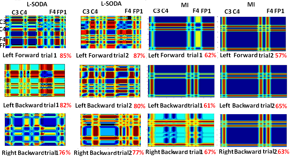
We used a heat kernel to transform (symmetrized) pairwise DI matrix into the distance matrix and applied K-means clustering to the distance matrix with the number of cluster (3) chosen by setting a threshold to within-cluster sums of point-to-centroid distances. For left hand forward movement, the three clusters were $(C_{3},C_{4},T_{3},T_{5})$, $(F_{4},FP1,FP2)$ and the rest of the electrodes. Mapping the EEG channels into Brodmann areas [25], we identified cluster $(C_{3},C_{4},T_{3},T_{5})$ as reflecting auditory processing such as that associated with detecting a cue to start motion (Brodmann area 21) and the execution of motor function (Brodmann area 4). Similarly, we identified cluster $(F_{4},FP1,FP2)$ as corresponding to the planning of complex movements (Brodmann area 8) and cognitive branching (Brodmann area 10). The third cluster corresponded to electrodes that were not very active. The localization accuracy was highlighted for each heatmap with red numbers in Fig. 1. In Fig. 1, the order of the electrodes by clustering were $T_{3}$, $T_{5}$, $C_{3}$, $C_{4}$, $T_{4}$, $F_{8}$, $CZ$, $F_{7}$, $F_{3}$, $T_{6}$, $PZ$, $P_{3}$, $P_{4}$, $O_{1}$, $O_{2}$, $FZ$, $F_{4}$, $FP_{1}$, $FP_{2}$ from left to right and from top to bottom. Compared to MI, L-SODA was more informative for localization with 10% improvement on average and is able to detect more accurate interactions when the same threshold of p-values was applied, where the localization accuracy has been highlighted along with the heatmap using red numbers. While MI and coherence measure [1][4] were not able to detect such interactions due to lower sensitivity to directional information flow.

Figure 2: Visual illustration of the dependencies between different electrodes for the activity ”left hand forward movement” reconstructed using Granger’s measure, unregularized DI by Quinn et al.[26], SODA and L-SODA averaged over the total 6 seconds, where the threshold for declaring an edge present corresponds to a p-value of level 0.05 which corresponds to the best localization accuracy shown in Table 1. The False Discovery Rate (FDR) is controlled below 0.1 using corrected BH procedure to resolve the multiple comparison problem and the sliding window width is $T=7$. Again, L-SODA detects more interactions compared to MI, Granger’s measure and unregularized DI. For instance, the edges between $(FP_{1}\rightarrow F_{4})$ and $(FP1\rightarrow FZ)$ corresponding to p-values of level 0.027 and 0.035 respectively using L-SODA. These interactions cannot be discovered by other approaches. The red dot arrows are false positives with unregularized DI by Quinn et al.[26] validated by neural pathway locations and Brodmann area, where the channels denoted as false positives do not have motor-related functions.

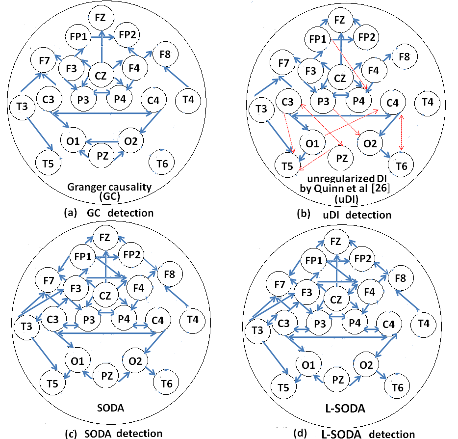
Comparison: Fig. 2 compared interaction graph discovery obtained through SODA with other state-of-the-art approaches using the activity ”Left Hand Forward Movement”. These results were representative but, due to space limitations, the interaction graphs for other motor activities are not discussed here. The regions in the brain for Fig. 1 that exhibit the highest activity match perfectly with the regions in Fig. 2 that have densest number of links. Fig. 2 indicated that L-SODA discovered significantly more interactions where the sliding window size is $T=7$. These new interactions can be validated by the fact that p-values are significant. For instance, the edges between $(FP1\rightarrow F_{4})$ and $(FP1\rightarrow F_{7})$ corresponded to p-values of level 0.027 and 0.035 respectively. The results of applying SODA on the replicates of EEG signals also indicated that during these periods, the electrodes $FP1$, $F_{4}$ and $F_{7}$ were highly interactive and therefore can serve as strong evidence that the activity was indeed being localized to these electrodes in the brain associated with motor control. Compared to the unregularized DI [26], L-SODA has the advantage that it can control false positive rate more accurately and its predictions are validated by neural pathway locations as determined by Brodmann areas. The main reason that L-SODA has the superior performance compared to the unregularized DI [26] is because the unregularized DI may underestimate the DI in the presence of small number of samples and high dimensional signals.

Figure 3: Illustration of DI as compared to MI for capturing similarities between activities for six pairs of EEG signals from different sources of electrodes in BCI project dataset such as $(C_{3},O_{1})$, $(FP_{1},FP_{2})$. As it is a directional measure, DI is more sensitive than MI to the emergence of the mental task and this can be seen from the fact that the peak of red $\Delta$DI trajectory is sharper than the peak of the blue $\Delta$MI trajectory over time. ($\Delta$DI is the temporal change of the DI similarity measure over successive temporal segments and similarly for $\Delta$MI). The dashed vertical lines correspond to the beginnings of the activities.

Figure 4: Visual illustration of electrodes by applying multidimensional scaling on the heatmaps and reducing the dimensions into 2 with L-SODA and MI for different activities, where the blue and red curves represent the first dimension and the second dimension. The horizontal axis in the figure represents the electrodes and the vertical axis represents the amplitudes. By comparing these dependency scatterplots to the spatial organization of the electrodes, interesting patterns are identified for different activities. For instance, the electrodes $C_{3}$ and $C_{4}$, $T_{3}$ and $T_{5}$ have strong interactions for left hand forward movement. Some of the representative traces are shown in Fig. 3.

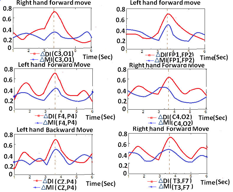
In Fig. 3 we plot the local DI and local MI as time trajectories. These trajectories can be interpreted as scan statistics for localizing interactions in the two EEG signals. Fig. 3 illustrated of the advantages of DI as compared to MI for capturing similarities between six pairs of EEG signals from BCI dataset. As shown in Fig. 3, DI is more sensitive than MI to the emergence of the mental task due to the fact that DI is a directional measure. The results show that DI can successfully detect highly interactive periods between pairs of electrodes corresponding to the temporal annotations in BCI dataset. Similar performance can be shown for the rest pairs of interactions in the total 19$\times$ 18=342 pairs of possible interactions.
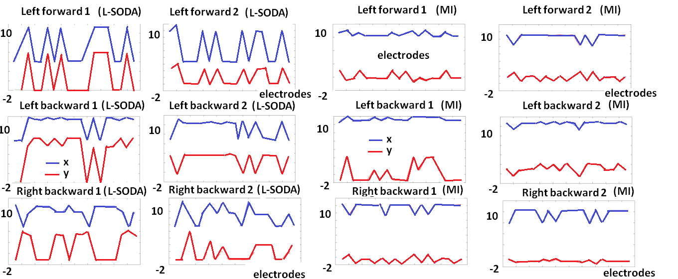
Spatial Pattern: To further reveal the spatial patterns of the electrodes, in Fig. 4, we show visual illustration of 2D scatter plots of electrodes by applying multidimensional scaling on the heatmaps and reducing the dimensions into 2 with L-SODA and MI for different activities, where the blue curve represented the first dimension and the red curve represents the second dimension. By comparing these dependency scatterplots to the spatial organization of the electrodes, interesting patterns were identified for different activities. For instance, the electrodes $C_{3}$ and $C_{4}$, $T_{3}$ and $T_{5}$ had strong interactions for left hand forward movement.

Figure 5: Visual illustration of the dependencies between different electrodes for the activity ”left hand forward movement” reconstructed using L-SODA dynamically with 1 second interval, where the results demonstrate that the interactions first start from the regions close to C3 and C4 which is Somatosensory and Motor region, and then transmit to other regions in the human brain.

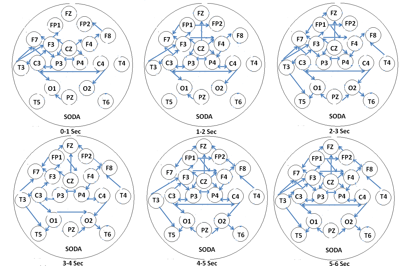
Dynamical Analysis: Besides the average localization and interaction detection performance, it was more desirable to reveal the dynamical process of the interaction between the EEG channels. To demonstrate the interactions among electrodes dynamically, Fig. 5 plots visual illustration of the dependencies between different electrodes for the activity ”left hand forward movement” reconstructed using L-SODA with 1 second interval, where the results demonstrated that the interactions first start from the regions close to C3 and C4 which is Somatosensory and Motor region, and then transmit to other regions in the human brain.

4.1.3 Consistency Measure

To study the ability of SODA to uncover interactions that were consistently observed during the same class of activity, we randomly divided the data into equal sized training and test sets. SODA was applied to the training set and the localization consistency was computed by mapping the detected interactions to the testing set. Table 1 demonstrated the comparison of the EEG localization accuracy of different algorithms using different levels of false discovery rates (FDR) including MI, Granger’s measure where the covariance matrix is regularized with Ledoit Wolf shrinkage method, coherence measure, unregularized DI of Quinn et al. and L-SODA. A localization consistency of 100% means that all interactions discovered on the training set were observed in the test set. As shown in Table 1, when the level of FDR was large, the five methods have comparable performance. When the threshold was lowered, L-SODA significantly outperforms other methods in localization accuracy. Since the weak dependencies were filtered out and strong dependencies remains with a lower threshold, false positives are reduced for all the five methods. Meanwhile, the hit using L-SODA remained to be high due to its non-symmetric measure. This explains the fundamental reason that L-SODA achieved the best performance with the threshold for declaring an edge present corresponding to a p-value of level 0.05. Compared to Granger’s measure and unregularized DI which were non-symmetric measures, L-SODA improved the accuracy by about 8% and 3% due to the fact that L-SODA was a shrinkage optimized version of directed information estimator for non-Gaussian distribution of the signals.

We also assessed localization consistency in terms of interactions within regions of the brain coordinating similar task related behavior (i.e., as opposed to between all EEG electrode sites). Using the corrected BH procedure [35] for L-SODA, 39 interactions were detected when FDR is equal to 0.1, while 24, 27 and 32 interactions were detected using MI, CM and unregularized DI. In Table 2, we identified electrodes that are either sources, recipients, or both sources and recipients of information flow from the second-by-second plots of the 19$\times$19 matrices. Table 3 demonstrated the Brodmann areas and the corresponding functions for the channels that are either sources, recipients, or both sources and recipients of information flow, where we identified that the directed information graph discovered by L-SODA is consistent with activation of the known Brodmann areas of the brain associated with motor functions. The comparison of the average running time for directed information between pairs of channels is reported in Table 4, where we demonstrate that L-SODA has the same order of computational complexity compared to the unregularized DI by Quinn et al.[26].

4.1.4 Classification

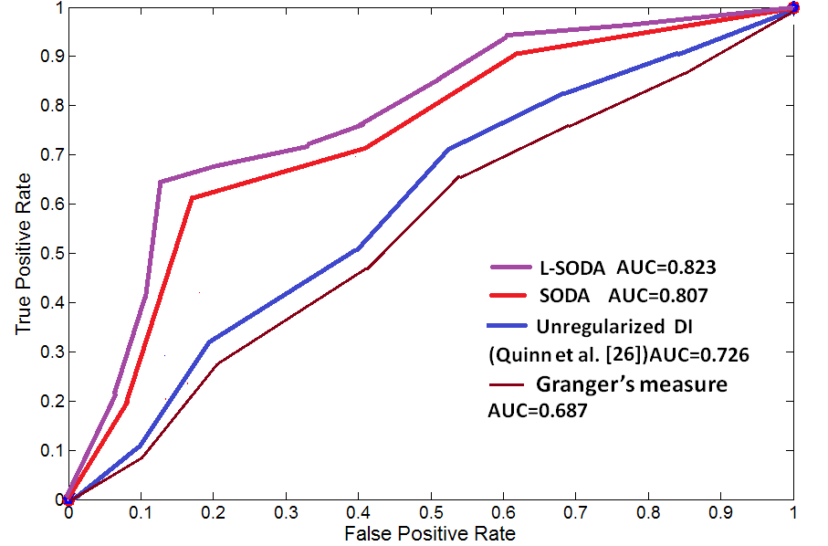
We next evaluated the classification performance of EEG signals using L-SODA as compared to MI and Hidden Markov Model (HMM) where the objective was to classify among the 10 classes of activities from the EEG data. The L-SODA classification task was conducted by applying the $k$ nearest neighbor classifier on the pair-wise distances computed using L-SODA. In Table 5 we compared the classification performance of L-SODA to that of the unregularized DI, the HMM implemented with GMM and Kernel-based Hidden Markov Model (HMM) where Gaussian radial basis function was utilized evaluated using EEG signals in the BCI project dataset. Table 5 indicated L-SODA outperforms HMM and unregularized DI in terms of EEG signal classification. This improvement may be attributed to the presence of model mismatch and bias in the HMM model as contrasted to the more robust behavior of the proposed model-free shrinkage DI approach. A more comprehensive quantitative comparison was shown in Table 6 with the mean and standard deviations for different activities. The superior performance of L-SODA compared to coherence measure and MI can be attributed to the fact that coherence measure and MI were symmetric measures and less sensitive in capturing the directional information flow between EEG signals such as the directed dependencies between ($T3\rightarrow F7$), ($T4\rightarrow F8$). Granger’s measure was based on a strong Gaussian model assumption, which may account for its inferior performance. In Fig. 6, we demonstrated the comparisons of ROC curves for classification performance with all the 10 classes of activities using L-SODA, SODA, Granger’s measure and unregularized DI by Quinn et al.[26], where L-SODA significantly outperformed Granger’s measure and the unregularized DI by Quinn et al.[26] in terms of area under the curve (AUC). L-SODA achieved the AUC 0.823, Granger’s measure achieved the AUC 0.687 and the unregularized DI achieves the AUC 0.726. L-SODA has 8% lower false negative rate (namely 8% higher in true positive rate) in detecting significant information flow at given level of false positives in terms of ROC curves, which can be mainly attributed to the fact that the use of optimized shrinkage regularization estimator in L-SODA.

Figure 6: Comparisons of ROC curves of classification performance for BCI dataset with all the 10 classes of activities using L-SODA, SODA, Granger’s measure and unregularized DI by Quinn et al.[26], where L-SODA significantly outperforms Granger’s measure and the unregularized DI by Quinn et al.[26] in terms of area of the curve (AUC).

FDR	0.1	0.07	0.05
MI	0.641	0.657	0.676
GC	0.653	0.705	0.728
CM	0.657	0.694	0.726
uDI	0.669	0.721	0.743
SODA	0.698	0.755	0.809
L-SODA	0.715	0.767	0.823

Table 1: Comparison of the EEG localization accuracy for different level of significance (false discovery rate), where the accuracy is computed by mapping the detection results using L-SODA on different replicates and the number of these electrodes that are connected in the MI, GC, CM, uDI, SODA and L-SODA interaction graphs, determined by thresholding these quantities at the same FDR level. uDI, CM and GC represents unregularized DI, coherence measure and Granger causality.

	0-1s	1-3s	3-4s	4-5s	5-6s
Send	FP2	FP2	$T_{4},F_{8}$	Null	Null
Send and Receive	$F_{8},T_{4},T_{5}$	$F_{8},T_{4}$	FP2	FP1,FP2,CZ	$T_{4},T_{5},F_{8},FP2,CZ$
Receive	FZ	$P_{3},T_{6}$	$P_{3},T_{6}$	$F_{3},F_{4},T_{3},T_{4},T_{5},F_{8}$	$T_{3}$

Table 2: Identification of the electrodes that are either sources, recipients, or both sources and recipients of information flow from the second-by-second plots in Fig. 5.

Channel	Brodmann Area	Function
FP2	right 10	executive function; tertiary motor (E)
$F_{8}$	right 44,45,46,47	grasping/manipulation; tertiary motor (G)
$T_{4}$	right 21	contemplating distance (C)
$T_{3}$	left 21	contemplating distance (C)
$CZ$	middle 5	maintain spatial reference for goal oriented behavior (MA)
$FP1$	left 10	executive function; tertiary motor (E)
$T_{5}$	left 19,37	motion sensitive visual processing; contemplating distance (MO)
$F_{3}$	left 8	planning of complex movements (P)
$F_{4}$	right 8	planning of complex movements (P)
$T_{6}$	right 19,37	motion sensitive visual processing; contemplating distance (MO)

Table 3: The Brodmann areas and the corresponding functions for the channels that are either sources, recipients, or both sources and recipients of information flow from the second-by-second plots in Fig. 5.

	unregularized DI by Quinn et al.[26]	L-SODA
CPU time (sec)	0.12	0.15

Table 4: Comparisons of the average running time for directed information between pairs of channels using L-SODA and unregularized DI by Quinn et al.[26] for BCI dataset, where L-SODA and unregularized DI have the same order of computational complexities.

	HMM(n=2)	HMM(n=5)	HMM(n=7)	KHMM [14]
AP	0.645	0.683	0.712	0.749
	MI	unregularized DI	SODA	L-SODA
AP	0.661	0.768	0.815	0.826

Table 5: Comparisons of Average Precision (AP) for EEG signal classification for logit shrinkage optimized directed information assessment (L-SODA), SODA, unregularized DI, Hidden Markov Model (HMM) with Gaussian mixture model (GMM) ($n$ is the number of components) and kernel-based Hidden Markov Model (KHMM), where the average precision is calculated by averaging the classification accuracy over all the activities. Ground truths correspond to the labels for 10 different types of activities.

Task	Left Hand Forward [%]	Right Hand Forward [%]	Left Leg [%]	Right Leg [%]
Granger’s measure	69.3$\pm$ 5.3	72.5$\pm$ 3.6	67.6$\pm$ 2.1	63.5$\pm$ 2.6
Coherence Measure[1]	73.5$\pm$ 2.7	74.1$\pm$ 4.2	68.1$\pm$ 8.3	65.8$\pm$ 5.1
Mutual Information	65.1$\pm$ 2.9	65.9$\pm$ 3.0	63.0$\pm$ 11.3	62.5$\pm$ 3.8
Quinn et al’s DI [26]	72.1$\pm$ 4.0	75.6$\pm$ 2.3	70.3$\pm$ 8.5	67.9$\pm$ 6.9
SODA	81.3$\pm$ 4.6	81.7$\pm$ 2.5	76.1$\pm$5.8	77.5$\pm$ 4.3
L-SODA	82.5$\pm$ 5.1	83.1$\pm$ 4.5	78.2$\pm$ 4.7	79.5$\pm$ 3.3

Table 6: Percentages (mean and standard deviations) of correctly recognized single trials for the different activities for Project BCI dataset. L-SODA gives at least 6% improvement in average precision over the best alternative Quinn et al’s regularized DI and L-SODA has roughly similar performance compared to SODA. The $k$ nearest neighbor classifier is implemented for classification.

4.2 CHB-MIT Scalp EEG Database

The CHB-MIT Scalp EEG Database, collected at the Children’s Hospital Boston, consists of EEG recordings from pediatric subjects with intractable seizures. Subjects were monitored for up to several days following withdrawal of anti-seizure medication in order to characterize their seizures and assess their candidacy for surgical intervention. All signals were sampled at 256 samples per second with 16-bit resolution. The recordings, grouped into 23 cases, were collected from 22 subjects. Different from BCI dataset, the CHB-MIT Scalp EEG Database has the annotations of the beginning and the ending time of the onset of seizure. The main task associated with the database is seizure detection. There are three performance metrics of interest. The electrographic seizure onset detection latency $EO_{latency}$ corresponds to the delay between electrographic onset and detector recognition of seizure activity. The sensitivity represents to the percentage of test seizure identified by a detector. The false alarm per hour is the number of times, over the course of an hour, that a detector declares the onset of seizure activity in the absence of an actual seizure. Generally, the goal of seizure detection is to signal an alert within 10 seconds of seizure onset. The non-seizure vectors are computed from at least 24 hours of nonseizure EEG, where both of awake and sleep status for non-seizure EEG are included. In our work, we compared the use of L-SODA to the best known seizure detector based on Shoeb et al. [42]. The approach of Shoeb et al. uses energy-based features obtained by passing the EEG signals through $M$-band filterbank $(M=8)$ through 0.5-24Hz and measuring the energy in the subband signals. In our experiments, detection was formulated as a binary classification problem (seizure vs. non-seizure) and implemented with support vector machine (SVM) classification. In order to formulate the L-SODA feature vector, we pre-processed the data by using a bandpass filter from 0.5 to 70 Hz, with a notch filter at 59-61 Hz to remove line noise. Subsequently, we applied multidimensional scaling (MDS) on the distance matrices estimated by L-SODA to reduce them to 2 dimensions. The SVM used by the detector is trained using the LibSVM software package with a cost factor $J=1$, RBF kernel parameter of $\gamma=0.1$ and trade-off between classification margin and error $C=1$ with 2-fold cross-validation.

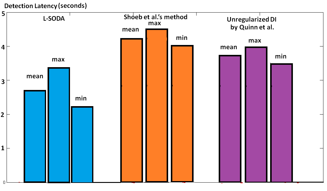
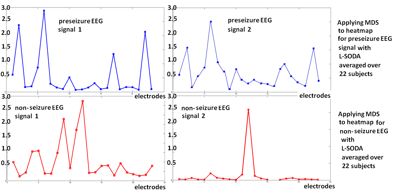
Overall, 97.1% out of the 173 test seizures were detected using L-SODA, which was slightly better than the energy-based method by Shoeb et al. with 96%. The mean latency with which the L-SODA detector declared seizure onset was 2.8 seconds. We demonstrate in Fig. 7 the comparison of the mean, minimum and maximum detection latency for pre-seizure data using L-SODA, the method by Shoeb et al. [42] and unregularized DI by Quinn et al. [26], where L-SODA had the shortest detection latency due to its sensitivity for temporal changes of EEG signals. In Fig. 8 we demonstrated the comparison of the results for applying MDS to heatmaps for pre-seizure and non-seizure EEG signals where the result was averaged over 22 subjects and the pre-seizure data represents the scalp EEG signal within 10 seconds before the onset of seizure where the vertical axis represented the amplitude and the horizontal axis represents the electrodes. As shown in Fig. 8, the patterns identified by L-SODA for pre-seizure and non-seizure EEG signals were significantly different, which resulted in accurate prediction when SVM is implemented. In Fig. 9, we demonstrated that comparison of false detections for the patient-specific detector using L-SODA, unregularized DI by Quinn et al. and energy-based method by Shoeb et al. where $x$ axis represented the patient number and $y$ axis represents the number of false detections. While we found that all of the three methods can achieve high positive rates, as shown in Fig. 9, the proposed L-SODA with logistic regression have reduced the number of false detections compared to unregularized DI by Quinn et al. [26] and Shoeb et al.’s energy feature-based method especially for the patients 1, 6, 12, 13, 15, 16 and 17. The superior performance can be mainly attributed the fact that the L-SODA is more sensitive in capturing the patterns of directional information flow while the energy feature-based feature described by Shoeb et al. does not account for the temporal dependency of the EEG signals. Therefore, their method misses or has a large detection latency when a test seizure differs significantly in spatial or spectral character from all of the seizures in the training set.

Figure 7: Comparison of the mean, minimum and maximum of detection latency (seconds) for pre-seizure data using L-SODA, the method by Shoeb et al. [42] and unregularized DI by Quinn et al. [26].

Figure 8: Comparison of the results for applying multi-dimensional scaling (MDS) to heatmaps for pre-seizure and non-seizure EEG signals, where the result is averaged over 22 subjects and the pre-seizure data represents the scalp EEG signal within 10 seconds before the onset of seizure. The vertical axis represents the amplitude and the horizontal axis represents the electrodes.

Figure 9: Comparison of false detections for seizure data using the patient-specific detector with L-SODA, unregularized DI by Quinn et al. [26] and energy-based method by Shoeb et al. [42] where $x$ axis represents the patient number and $y$ axis represents the number of false detections.

Conclusion

We proposed a novel non-parametric model-free framework called L-SODA for EEG signal interaction detection and classification based on directed information. L-SODA uses a new James-Stein shrinkage approach to logistic regression of directed information estimation resulting in minimum mean squared error. A central limit theorem for the L-SODA estimator specifies p-values that can be used to filter out false positive peaks of the estimated L-SODA. We illustrated the L-SODA estimator for EEG signals interaction detection/localization and classification using BCI databases. L-SODA provides interaction estimated that are consistent with neural pathway locations as determined by Brodmann areas. Our results indicate that L-SODA is able to detect interaction regions in human brains that involve strong directional information flow without imposing strong model assumptions. Since L-SODA captures the directional information that EEG signals naturally possess and successfully controls the overfitting error with optimized shrinkage regularization, L-SODA demonstrates better performance as compared to unregularized DI and undirected methods such as MI or coherence measure methods. Moreover, we evaluated the L-SODA on CHB-MIT Scalp EEG database for seizure detection. We demonstrated that compared to the state-of-the-art approaches, the proposed method provides better performance in detecting the epileptic seizure.

Reference

[1] G. Nolte, O. Bai, L. Wheaton, Z. Mari, S. Vorbach and M. Hallett, Identifying true brain interaction from EEG data using the imaginary part of coherency, Clinical Neurophysiology, Vol 115, Issue 10, 2004.

[2] Baccala LA and Sameshima K. Partial directed coherence: a new concept in neural structure determination. Biological Cybernetics, Vol 84, No 6, 2001.

[3] L. Wu, P. Neskovic, E. Reyes, E. Festa, and W. Heindel, Classifying n-back EEG data using entropy and mutual information features, European Symposium on Artificial Neural Networks, 2007.

[4] L. Tian, D. Erdogmus, A. Adama, and M. Pavel, Feature selection by independent component analysis and mutual information maximization in EEG signal classification, IEEE International Joint Conference on Neural Network, 2005.

[5] J. Hausser and K. Strimmer, Entropy inference and the James-Stein estimator, with application to nonlinear gene association networks, Journal of Machine Learning Research, Vol 10, No 12, 2009.

[6] T. Yan, J. Tang, A. Gong and W. Wang , Classifying EEG Signals Based HMM-AR, International Conference on Bioinformatics and Biomedical Engineering, 2008.

[7] P. Ferrez and J.  Millan, EEG-Based Brain-Computer Interaction: Improved Accuracy by Automatic Single-Trial Error Detection, Advances in Neural Information Processing System, 2007.

[8] L. Wu and P. Neskovic, Feature extraction for EEG classification: representing electrode outputs as a Markov stochastic process, European Symposium on Artificial Neural Networks, 2007.

[9] W. Xu, C. Guan, C. Siong, S. Ranganatha, M. Thulasidas and J. Wu, High Accuracy Classification of EEG Signal, in International Conference on Pattern Recognition, 2004.

[10] A. Rao, A. Hero, D. States, and J .Engel, Using Directed Information to Build Biologically Relevant Influence Networks, in Journal on Bioinformatics and Computational Biology, Vol. 6, No.3, June 2008.

[11] B. Blankertz, G. Curio, and K .Muller, Classifying single trial EEG: Towards brain computer interfacing, Advances in Neural Information Processing System, 2002.

[12] G. W. Oelhert, A note on the Delta method, The American Statistician, Vol. 46, No 1, 1992.

[13] D. Garrett, D. Peterson, C. Anderson and M. Thaut, Comparison of linear, nonlinear, and feature selection methods for EEG signal classification, Vol 11, No 2, IEEE Transactions on Neural Systems and Rehabilitation Engineering, 2003.

[14] W. Xu, J. Wu, Z. Huang and C. Guan, Kernel Based Hidden Markov Model With Applications to EEG Signal Classification, The IASTED Int. Conf. on Biomedical Engineering, 2005.

[15] M. Krumin and S. Shoham. Multivariate autoregress modeling and granger causality analysis of multiple spike trains. Computational Intelligence and Neuroscience, 2010.

[16] J. Massey. Causality, feedback and directed information. Symp Information Theory and Its Applications (ISITA), 1990.

[17] Project BCI - EEG motor activity dataset, http://sites.google.com/site/projectbci/, Brain Computer Interface research at NUST Pakistan.

[18] J. Cohen, W. Peristein, T. Braver, L. Nystrom, D. Noll, J. Jonldes and E. Smith, Temporal dynamics of brain activation during a memory task, Nature, Vol 386, 1997.

[19] H. Meleis1, S. Takashima1 and R. Harner, Analysis of inphase interaction pattern in EEG, Bioelectromagnetics, Volume 3, Issue 1, 1982.

[20] H. Hui, D. Pantazis, S. Bressler, and R. Leahy, Identifying True Cortical Interactions in MEG using the Nulling Beamformer, Neuroimage, 49(4), 2010.

[21] K. Ang, Z. Chin, H. Zhang, and C. Guan, Mutual information-based selection of optimal spatial-temporal patterns for single-trial EEG-based BCIs, Pattern Recognition, 2011.

[22] L. Almeida, MISEP - Linear and nonlinear ICA based on mutual information, Journal of Machine Learning Research, 4, 2004.

[23] W. Hesse, E. Moller, M. Arnold and B. Schack, The use of time-variant EEG Granger causality for inspecting directed interdependencies of neural assemblies, Journal of Neuroscience Methods, 124(1), 2003.

[24] A. Delorme, Makeig and S. EEGLAB, an open source toolbox for analysis of single-trial EEG dynamics, Journal of Neuroscience Methods, 134:9-21, 2004.

[25] http://start.eegspectrum.com/Newsletter/.

[26] Quinn, C.J. and Coleman, T.P. and Kiyavash, N. and Hatsopoulos, N.G, Estimating the directed information to infer causal relationships in ensemble neural spike train recordings, Journal of computational neuroscience, 30(1), 2011, Springer.

[27] Supp, G.G. and Schlogl, A. and Trujillo-Barreto, N. and Muller, M.M. and Gruber, T., Directed cortical information flow during human object recognition: analyzing induced EEG gamma-band responses in brain’s source space, PLoS One, 2(8), 2007.

[28] Hinrichs, H. and Noesselt, T. and Heinze, H.J., Directed information flow-A model free measure to analyze causal interactions in event related EEG-MEG-experiments, Human brain mapping, 29(2), 2008.

[29] Babiloni, F. and Cincotti, F. and Babiloni, C. and Carducci, F. and Mattia, D. and Astolfi, L. and Basilisco, A. and Rossini, PM and others, Estimation of the cortical functional connectivity with the multimodal integration of high-resolution EEG and fMRI data by directed transfer function, Neuroimage, 24(1), 2005.

[30] Astolfi, L. and Cincotti, F. and Mattia, D. and Marciani, M.G. and Baccala, L.A. and de Vico Fallani, F. and Salinari, S. and Ursino, M. and Zavaglia, M. and Ding, L. and others, Comparison of different cortical connectivity estimators for high-resolution EEG recordings, Human brain mapping, 28(2), Wiley Online Library, 2007.

[31] Korzeniewska, A. and Maczak, M. and Kamiski, M. and Blinowska, K.J. and Kasicki, S., Determination of information flow direction among brain structures by a modified directed transfer function (dDTF) method, Journal of neuroscience methods, 125(1-2), Elsevier, 2003.

[32] Lotte, F. and Congedo, M. and Lécuyer, A. and Lamarche, F. and Arnaldi, B., A review of classification algorithms for EEG-based brain–computer interfaces, Journal of neural engineering, 4, IOP Publishing, 2007.

[33] Benjamini, Y. and Hochberg, Y., Controlling the false discovery rate: A practical and powerful approach to multiple testing, J. Roy. Statist. Soc. Ser. B. 1995; 57:289-300.

[34] Schfer, J., and K. Strimmer, An empirical Bayes approach to inferring large-scale gene association net- works, Bioinformatics,Oct 2004.

[35] Y.  Benjamini and D.  Yekutieli, The control of the false discovery rate in multiple testing under dependency, The Annals of Statistics, Vol. 29, No. 4, 1165-1188, 2001.

[36] J.P. Romano, A.M. Shaikh and M. Wolf, Control of the false discovery rate under dependence using the bootstrap and subsampling, TEST, 17, 2008.

[37] X. Chen, A. Hero and S. Savarese, Multimodal Video Indexing and Retrieval using directed information, IEEE Transactions on Multimedia Special Issue on Object and Event Classification in Large-Scale Video Collections, to appear, Aug, 2011.

[38] H. Cai, S. Kulkarni, and S. Verd u, Universal entropy estimation via block sorting. IEEE Transactions on Information Theory, 50(7):1551-1561, 2004.

[39] J. Ziv, and A. Lempel, A Universal Algorithm for Sequential Data Compression. IEEE Transactions on Information Theory, 23(3):337-343, 1977.

[40] J. Pillow, J. Shlens, L. Paninski, A. Sher, A. Litke, E. Chichilnisky and E. Simoncelli. Spatio-temporal correlations and visual signaling in a complete neuronal population. Nature 454: 995-999, 2008

[41] B. Krishnapuram, L. Carin, M. Figueiredo and A. Hartemink, Sparse Multinomial Logistic Regression: Fast Algorithms and Generalization Bounds, IEEE Transactions on Pattern Analysis and Machine Intelligence, 2005.

[42] A. H.Shoeb, Application of Machine Learning to Epileptic Seizure Onset Detection and Treatment, MIT, PhD Thesis, 2009.

[43] Brodmann K. Vergleichende Lokalisationslehre der Grosshirnrinde. Leipzig : Johann Ambrosius Bart, 1909.