Zipf-Mandelbrot-Pareto model
for co-authorship popularity

Abstract

Each co-author (CA) of any scientist can be given a rank ($r$) of importance according to the number ($J$) of joint publications which the authors have together. In this paper, the Zipf-Mandelbrot-Pareto law, i.e. $J\propto 1/(\nu+r)^{\zeta}$ is shown to reproduce the empirical relationship between $J$ and $r$ and shown to be preferable to a mere power law, $J\propto 1/r^{\alpha}$. The CA core value, i.e. the core number of CAs, is unaffected, of course. The demonstration is made on data for two authors, with a high number of joint publications, recently considered by Bougrine (2014) and for 7 authors, distinguishing between their ”journal” and ”proceedings” publications as suggested by Miskiewicz (2013). The rank-size statistics is discussed and the $\alpha$ and $\zeta$ exponents are compared. The correlation coefficient is much improved ($\sim$ 0.99, instead of 0.92). There are marked deviations of such a co-authorship popularity law depending on sub-fields. On one hand, this suggests an interpretation of the parameter $\nu$. On the other hand, it suggests a novel model on the (likely time dependent) structural and publishing properties of research teams.

Thus, one can propose a scenario for how a research team is formed and grows. This is based on a hierarchy utility concept, justifying the empirical Zipf-Mandelbrot-Pareto law, assuming a simple form for the CA publication/cost ratio, $c_{r}=c_{0}\>log_{2}(\nu+r)$. In conclusion, such a law and model can suggest practical applications on measures of research teams.

In Appendices, the frequency-size cumulative distribution function is discussed for two sub-fields, with other technicalities

Keywords : ranking; Zipf-Mandelbrot-Pareto law; power laws; co-authorship; research topics; peer review journals; proceedings; co-author core

1 Introduction

One basic question in scientometrics concerns the number of relevant co-authors (CA) for the set of publications of some principal investigator (PI). This leads to examine the CA core index (Ausloos 2013), $m_{a}$, introduced on several grounds, including a statistical framework. Recall that the $m_{a}$-index is deduced from a plot of the number ($J$) of joint publications (NJP) of a PI with CAs ranked according to their rank ($r$) of importance; $r=1$ being the most prolific CA with the PI. It has been found (Ausloos 2013) that

$$J(r)=a/r^{\alpha},$$ (1)

which holds best when there are enough $J$ and CA. It holds as well if the publication list is broken into specific types of publications, i.e. in sub-fields (Bougrine 2014) or peer-review journals and proceedings (Miskiewicz 2013). Miskiewicz (2013) has much discussed the exponent $\alpha$ value which turns out to be scientist dependent, whence is a valid criterion for team work assessment. However, neither Miskiewicz nor Ausloos have provided a statistical physics-like model or any argument for the findings.

In the present paper, such a model is presented as an adaptation of Mandelbrot model for text appraisal. In order to present arguments in such a favor, the Bougrine (2014) data is first reexamined along the 3-parameter Zipf-Mandelbrot-Pareto (ZMP) law (Zipf 1949, Mandelbrot 1960, Pareto 1896, West & Deering 1995)

$$J(r)=b/(\nu+r)^{\zeta}.$$ (2)

Next, several other co-authorships are examined distinguishing between their publications in (peer review) journals or proceedings and in a few cases the research sub-fields.

Obviously, the ZMP distribution is a natural generalization of an inverse power law. The ZMP law leads to a curvature at low $r$ in a log-log plot (if $\nu$ is positive) and presents an asymptotic power law behavior at large $r$. Both $\alpha$ and $\zeta$ exponents must be greater than 1 for the distributions to be well-defined, greater than 2 for the mean to be finite, and greater than 3 for the variance to be finite. Note that the ZMP distribution has been applied in many contexts, e.g., in studies of scientific citations (Tsallis & Albuquerque 2000). In fact, another important aspect of the ZMP distribution is that it arises in the context of generalized statistical physics (Tsallis 1988).

Fitting the ZMP law is much more troublesome than fitting the Zipf hyperbolic law (Fairthorne 1969, Haitun 1982, Iszak 2006). Thus, a variant of the ZMP law, i.e. the 4-parameter relation

$$J(r)=c/(\eta+\lambda r)^{\mu}$$ (3)

has been also examined, for comparing the resulting precisions of the respective fits. Since nothing drastic has been found in the present case, some data and analysis is left in Appendix A for completeness.

In order to argue in favor of a ZMP model for co-authorship popularity,

• two PI cases are here below examined: one is H.E. Stanley (HES): he has more than 1400 publications, is a guru of statistical mechanics; his group website distinguishes between activities in several research sub-fields. HES lists more than 500 CA. The other is M. Ausloos (MRA); he has published a little bit less than 600 papers in international journals or proceedings with reviewers; MRA has more than 300 CA. Both PIs have worked in different research fields, sometimes overlapping. Remarkable fits to the hyperbolic law, Eq.(1), are available (Miskiewicz 2013, Bougrine 2014) for both PIs, - at least in the central $J(r)$ region. Deviations mainly exist in the extreme regions. Thus, it seems of interest to reexamine the data in a more parametrized way, along the ZMP law;

• several other authors (7) CA lists are also examined, beside HES and MRA, - distinguishing between their publications in journals or proceedings;

• finally, the largest publication lists, i.e. those of HES and MRA, can be broken into several research sub-fields; the ZMP law validity and fit parameter values are examined in such cases.

After this brief introduction serving as basic arguments, the $J(r)$ data of the co-authorship features is rank-size analysed, in Sect. 2, for both MRA and HES, and for 7 other authors in Sect.2.1 and in Sect.2.2 along the above the simple empirical laws, Eqs.(1)-(2), distinguishing between the different types of publications mentioned here above.

In Sect. 3, some discussion on the statistical aspects of these illustrative cases are presented, stressing the parameter $\nu$, beside the characteristic exponents, either for co-authored papers in journals or proceedings, Sect. 3.1 or according to envisaged sub-fields, Sect. 3.2. It is argued that the ZMP law should be further considered from a theoretical point of view., when examining so called king, vice-roy, queen and harem effects, in Sect. 3.3. Therefore, a novel model is presented on the structural and publishing properties of research teams, in Sect. 4. Thus, one can propose a (rather common sense, $\sim$ Ockam’s razor mode) scenario for how a research team is formed around a PI and grows with preferred CAs. This is based on a hierarchy utility concept assuming a simple form for the CA publication/cost ratio.

Some summary and a short conclusion are found in Sect. 5.

As mentioned, practical considerations on fit precision through either Eq.(2) or Eq.(3) are found in Appendix A. A thorough discussion on generalizing the main text considerations to ”sub-cores” of co-authors is found in Appendix B.

In fine, another type of display that the rank-size plots is of interest in order to remain in line with somewhat more conventional plots in bibliometrics, i.e. frequency-size plots. For a brief comparison with other types of displays, and for some completeness, the cumulative distribution function (CDF) of the number of co-authors as a function of NJP, is reported as examples and commented upon, for the case of two sub-fields of MRA, in Appendix C.

2 The data, fits, and statistical analysis

Figure 1: Log-log scale display of the rank-size relationship between the total number of joint publications either with HES or with MRA, for co-authors ranked by ”decreasing importance”; best fits (color lines) are shown for the power law and ZMP law. Note that black dash lines are fits correspond to ZMP taking into account a king and vice-roy effect, i.e. removing 2 data points at low rank as outliers

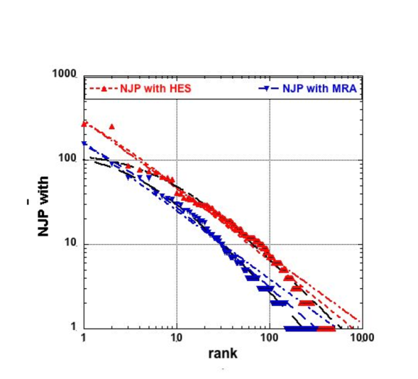
The $whole$ ($w$) joint publication list for the two prolific PIs with many CAs, i.e. HES and MRA, has been first studied, - the data being fitted with the best power law and best ZMP fits. The parameter values are reported in Table 1. The fits are rather remarkably good, both for the power law and the ZMP laws, with an R² above 0.94. The exponents are close to 1.0, as expected. The parameter values and the regression fit coefficient R² as given for the different cases have been rounded up to significant decimals.

Note that it is not surprising that all the numerical results slightly differ from those of Bougrine (2014). This is likely due to the type of algorithm used in these non linear fits. Bougrine (private communication) used a classical Least Squares curve fit, on log-log plots. In the present study, the fit is a non-linear one that uses the Levenberg-Marquardt algorithm. However, there is no disagreement on the qualitative conclusions. In fact, as mentioned, fitting the ZMP law is much more troublesome than fitting the Zipf hyperbolic law (Fairthorne 1969, Haitun 1982, Iszak 2006). However, the error bars on the parameter values, calculated from several simulations with different initial conditions, are less than 10%, - usually less 5%. For completeness, note that the quality of the fits were examined through the statistics of the errors (Jarqe & Bera 1980), i.e. whether the error distributions were relatively small and randomly distributed on the both side of the means. The worse cases occur when king and/or queen effects, see details below, are superposed to a power law tail, or when a strong exponential cut-off is present on the tail. Note also that fits in such cases necessarily imply large error bars on the amplitudes $a$, $b$, and $c$, since the number of CA having a given NJP can be large itself, the more so at high rank, when the number of publications with the PI, usually 1 or 2, is the same for many CAs.

It is well seen, on Fig.1, that a plot of the (whole) NJP data reveals a marked king effect both for MRA and HES, - even a king and vice-roy effect for HES. Thus, to emphasize the latter effect, the two lowest rank data points, the king and the vice-roy, have been removed before new fit attempts. The results are shown in Table 1 also, in HES* and MRA* lines. Observe that the major changes occur in the amplitudes, $\nu$ and $b$, - not in the fit exponents which rather indicate the asymptotic regime; note that $R^{2}$ goes from 0.92 to 0.99 for HES.

2.1 Peer-review journals and proceedings

A reviewer of the first submitted version of this report pointed out that (I quote) ”picking such singular authors allow a better statistic, …”. Indeed that is a relevant point. In fact, one tends in physics to look for large numbers, in view of finding some ”universality”, - but not many authors have so many papers as HES or MRA. For analysis consistency, I had taken the data in Bougrine (2014) publication. Nevertheless, it is of interest to look for less prolific authors, as pointed out by the reviewer. Thus, I have requested from reliable colleagues, having worked in statistical and/or condensed matter physics, some pertinent data. However, as an additional ”constraint”, I have asked such colleagues not to break their publication list into sub-fields, as Bougrine (2024) did, but rather to break their publication list into ”peer-review journals” and ”peer-review (or not) proceedings”, as Miskiewicz (2013) has investigated. No need to say that proceedings papers are often peer reviewed as well, but the distinction, as the one Miskiewicz proposed, is surely obvious to or acceptable by many.

Therefore, this leads to Table 1 and to many possible plots, - only a few are shown such that some emphasis is placed on major features or findings, Figs. 2, 3, and 4. Note that PIs are ranked according to NDCA rather than NJP, for better emphasis of PI popularity hierarchy than productivity, in Table 1.

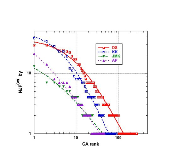
In Fig. 2, a log-log scale display of the whole set of joint publications (NJP^(w)) number by various (3) authors (see insert: DS, KK, JMK, AP) with different production outputs and is shown with co-authors (CA) ranked by decreasing importance”. Note that $R^{2}\simeq 0.98$, except for JMK (seeTable 1). Observe also a king effect for JMK, but the data has not been further analyzed, as for HES and MRA; if done, i.e. removing the king, it should surely markedly improve the $R^{2}$ coefficient, actually 0.95.

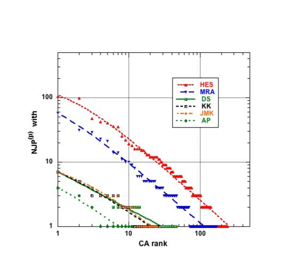
In Fig. 3, co-authors are ranked on the x-axis in decreasing order of their number of publications, in proceedings, with the 2 two ”main” PIs and 5 other PIs in statistical physics. It is seen that the ZMP law holds for such a type of publications, as well, - with marked king and queen effects.

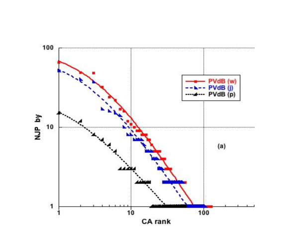
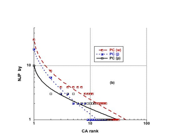
In contrast, the display of Fig. 4 shows a comparison of various types of publications by one author (PC), pointing out to a marked king effect, whatever the publication type, and another comparison of publication types with co-authors (PVdB) where marked queen effect is seen. At this point, it is sufficient to know that PVdB is an experimentalist working in condensed matter.

Thus, the various types of behaviors have been illustrated for various types of publications, indicating the ZMP framework interest. The values of the fit parameters, reported inTable 1, can be discussed in Sect. 3.

2.2 Sub-field effects

Next, let it be recalled that the NJP analysis was suggested by Bougrine (2014) to be breakable into sub-fields: e.g., into 12 appropriate sub-fields, for HES, here called $s_{i}$, and into 8 sub-fields, in the case of MRA, here called $a_{i}$, - according to the web site of such authors. For coherence, the same set of sub-fields has been used here. Let it be recalled that for justified statistical purposes, Bougrine has also merged some $s_{3}$ and $s_{6}$ into some $s_{63}$ and some $a_{4}$ and $a_{5}$ into some $a_{54}$. The same is done here; names of sub-fields are presently irrelevant. Two specific cases, i.e. $a_{2}$ and $a_{7}$ (they refer to work on Magnetic Materials and Superconductivity, respectively) will be examined in Appendix B and in Appendix C, as mentioned in the Introduction, i.e. for comparing the size-rank method with the size-frequency method.

The hyperbolic law, Eq. (1) has been studied on all $s_{i}$ and $a_{i}$ data; numerical results reported in Table 2. The law is often well obeyed, since R² $\in\sim[0.88,0.99]$, - except for $s_{4}$, in which case R${}^{2}\sim 0.787$. Observe that the cases with the ”worse” exponent, i.e. $\alpha$ rather away from +1 in $s_{9}$ and $a_{6}$, correspond to the $oldest$ sub-fields of investigations both for HES, i.e. phase transitions and critical phenomena, and for MRA, i.e., kinetic growth and spin models, - in fact, two closely related sub-fields! An open question is whether such a variation is due to time effects or to sub-field distinctions.

The 3 parameter ZMP (3-ZMP) law necessarily leads to a better R², except for $s_{3}$ and $a_{5}$ which are almost unchanged with respect to the hyperbolic law. Recall that they belong to data sets with very low numbers of CAs and NJP. All other R² values move close to 0.98 or above from $\sim$ 0.92 on average for the power law.

The values of the fit parameters will be discussed in Sect. 3.

				3 param. ZMP, Eq.(2)					power law, Eq.(1)
PI	NJP	NDCA	$<$NCA$>$	$b$	$\nu$	$\zeta$	R2		$a$	$\alpha$	R2
HES (w)	1148	592	6.57	335.0	0.10	0.83	0.92	-	314.	0.81	0.92
HES∗ (w)	*	*	*	1128.0	7.384	1.098	0.987	-	246.9	0.765	0.96
HES (j)	791	568	4.67	186.0	-0.10!	0.78	0.94	-	200	0.80	0.94
HES (p)	296	242	5.15	255.4	1.34	1.0	0.97	-	119.	0.76	0.95
MRA (w)	599	319	4.87	276.25	0.88	0.97	0.99	-	161.9	0.81	0.98
MRA∗ (w)	*	*	*	723.3	4.149	1.203	0.988	-	207.2	0.894	0.96
MRA (j)	359	273	3.86	183.4	1.02	0.95	0.99	-	101.7	0.78	0.98
MRA (p)	164	128	3.04	87.78	0.58	0.94	0.99	-	59.67	0.81	0.98
DS (w)	612	280	2.72	953.1	10.56	1.38	0.98	-	43.18	0.62	0.85
DS (j)	374	268	2.58	637.0	9.52	1.31	0.98	-	38.74	0.62	0.86
DS (p)	59	46	1.57	7.04	-0.01!	0.58	0.96	-	7.08	0.58	0.96
PVdB (w)	99	129	4.25	529.2	3.15	1.44	0.99	-	76.4	0.82	0.94
PVdB (j)	73	105	3.82	296.8	2.485	1.38	0.975	-	58.3	0.83	0.94
PVdB (p)	26	56	2.14	40.7	1.47	1.07	0.98	-	16.6	0.75	0.96
KK (w)	172	93	6.01	1085.1	6.21	1.67	0.985	-	47.02	0.735	0.90
KK (j)	144	85	5.66	1191.4	6.77	1.72	0.986	-	41.79	0.732	0.90
KK (p)	28	28	2.79	10.20	0.65	0.765	0.946	-	7.21	0.635	0.94
AP (w)	111	47	2.87	35.61	0.72	0.98	0.98	-	21.81	0.80	0.98
AP (j)	79	45	2.62	42.21	1.27	1.07	0.98	-	18.50	0.78	0.96
AP (p)	9	11	1.55	4.74	0.21	0.78	0.93	-	4.11	0.71	0.93
JMK (w)	60	41	2.71	27.45	1.57	0.87	0.95	-	13.17	0.63	0.94
JMK (j)	28	35	1.71	23.50	2.54	1.00	0.93	-	7.165	0.60	0.89
JMK (p)	19	25	2.04	15.47	1.50	0.88	0.97	-	7.34	0.61	0.95
PC (w)	33	32	3.09	8.18	-0.90!	0.56	0.99	-	28.32	1.25	0.94
PC (j)	22	19	2.68	6.59	-0.78!	0.74	0.99	-	19.53	1.41	0.98
PC (p)	10	24	2.0	3.89	-0.91!	0.40	0.96	-	8.93	0.78	0.89
JM (w)	27	15	1.80	2.24	-0.97!	0.49	0.99	-	11.75	1.87	0.92
JM (j)	15	13	1.77	2.23	-0.95!	0.515	0.99	-	9.70	1.63	0.92
JM (p)	3	3	1.33	(-)	(-)	(-)	(-)	-	1.96	0.75	0.93

Table 1: Summary of fit parameters to NJP data corresponding to Figs.2-4 for various PIs, distinguishing between their whole (w) publication list and their papers published in journals (j) or in proceedings (p); the parameter values correspond to the various formulae discussed in the text, Eqs.(1)-(2); the regression fit coefficient R² is given for the different cases; data has been rounded up to significant decimals; error bars $\leq$ 10%; NDCA : number of different CAs; $<$NCA$>$: number of co-authors on average on a paper by the ”main” author (PI); for HES* and MRA*, see text

	3 param. ZMP, Eq.(2)				2 param. law, Eq.(1)
NJP	$\nu$	$b$	$\zeta$	R2	$a$	$\alpha$	R2
$s_{1}$	0.674	27.493	0.838	0.988	18.71	0.707	0.983
$s_{2}$	7.441	2434	2.074	0.978	33.05	0.740	0.885
$s_{4}$	12.12	4.6 105	$q.pw.t$	0.940	49.935	0.841	0.787
$s_{9}$	3.813	35.13	0.859	0.961	10.801	0.522	0.930
$s_{11}$	0.956	25.692	0.989	0.974	13.801	0.754	0.964
$s_{5}$	6.77	2003.9	$1.68$	0.979	76.78	0.737	0.886
$s_{7}$	0.196	74.116	1.054	0.994	61.99	0.982	0.994
$s_{8}$	1.172	90.31	1.128	0.982	40.13	0.844	0.972
$s_{10}$	4.221	579.37	1.427	0.982	63.09	0.756	0.920
$s_{12}$	3.157	357.47	$1.19$	0.987	77.70	0.731	0.928
$a_{1}$	2.59	28.478	1.088	0.939	7.694	0.637	0.908
$a_{2}$	20.77	2.9 104	$q.pw.t$	0.980	22.755	0.59	0.823
$a_{3}$	0.365	17.029	0.893	0.971	13.164	0.793	0.969
$a_{6}$	-0.438	19.771	1.199	0.988	39.324	1.62	0.980
$a_{7}$	0.274	144.34	0.925	0.981	118.2	0.859	0.980
$a_{8}$	5.446	665.2	1.852	0.971	23.348	0.744	0.900
$s_{3}$	0.665	9.726	0.989	0.911	5.967	0.755	0.910
$s_{6}$	5.821	$exp.t$	$exp.t$	$0.970$	14.12	0.914	0.908
$s_{63}$	8.09	$exp.t$	$exp.t$	$0.970$	14.37	0.764	0.890
$a_{4}$	2.51	61.69	1.427	0.969	10.932	0.781	0.940
$a_{5}$	-0.594	2.708	0.425	0.895	3.860	0.612	0.888
$a_{54}$	-0.022	13.764	0.844	0.989	14.00	0.852	0.989

Table 2: Summary of fit parameters to NJP data grouped as for Figs. 5-8; the parameters correspond to the various formulae discussed in the text, Eqs. (1)-(2); $q.pw.t$ indicates a strong queen plus power law tail effect and $exp.t$ indicates a strong exponential tail cut-off, i.e. cases for which the scaling parameters have large error bars; the regression fit coefficient R² is given for the different cases; data has been rounded up to significant decimals; error bars much below 10%

Figure 2: Log-log scale display of the number of all joint publications (NJP^(w)) by various authors (see insert: DS, KK, JMK, AP) with co-authors (CA) ranked by decreasing ”importance”; best fits (color lines) are shown for the ZMP law, Eq.(2)

Figure 3: Log-log scale display of the number of joint publications (NJP^(p)) in ”proceedings”, by various authors (see insert) with co-authors ranked by decreasing ”importance”; best fits (color lines) are shown for the ZMP law, Eq.(2)

Figure 4: Log-log scale display of the number of (various types of) joint publications (NJP) by (a) PVdB and (b) PC, with co-authors (CA) ranked by decreasing ”importance”; best fits (color lines) are shown for the ZMP law, Eq.(2); note the ”queen effect” in (a) and the ”king effect” in (b)

3 Amplitudes and exponents. A discussion

After the statistical analysis based on the correlation coefficient, $R^{2}$, let the exponent and amplitudes of the empirical laws be examined. first, reconsider the $whole$ data for the two PIs, HES and MRA, displayed with the best power law and best ZMP fits on Fig. 1. The ZMP is visually much better performing, - the more so if the two lowest ranked data points are removed before a fit to Eqs. (1)-(2). The display emphasizes that both HES and MRA have at least two privileged CAs. This is also going to be emphasized through the display in Figs. 2-4, irrespective of the ”very” or ”less” plowed research sub-fields.

Observe that such a removal of two outliers, induce a huge change (almost a factor of 3) in the amplitude $b$ and in $\nu$, thereby strongly stressing a queen affect , - due tot he king and vice-roy of HES, and the king of MRA. These effects on $\zeta$ are mild, though in both cases increase $\zeta$, indicating a faster decay of the empirical law at high rank, - in other words, a weakening of the role of the rare CAs.

3.1 Journals

From Table 1, it appears that the range of amplitude can be large and exponents rather narrow. The former is due to the wide range in the number of publications of various PIs, but the latter indicates some stability thus a reasonable guess of the empirical law, - in fact, as should be stressed, whatever the type of publication. Most of the values of $zeta$ are close to 1. The notable exceptions, pointing to non-universality in contrast indicate the interest of using such an exponent as a measure of the PI relationship with his/her team of CAs. Obviously, the greater the exponent $\zeta$ the shorter is the team size. The popularity is influenced by the number of rare CAs, thus by a widening of the NJP distribution,thus by a flattening of the tail, whence by a smaller $\zeta$ exponent.

Nevertheless, one should disregard the PIs who are in fact ”not quite PIs”, as exemplified by their small number of publications, and the value of $\nu$ being negative, i.e. PC and JM.

In so doing, the most popular PIs in the presently examined set are (in terms of the $\zeta$ exponent for the whole set of joint publications) : HES (0.83), JMK (0.87), MRA (0.97) and AP (0.98). It is thus very interesting to notice that neither DS (1.38) and KK (1.67) nor PVdB (1.44) are ”popular”. However, they have large ”harem”, - $\nu$ being quite large. This seems quite understandable due to the activities of the researchers.

Practically, it can be observed that HES presents a king and a vice-roy effect in NPJ^(j). Indeed the list of publications of HES shows the high relevance of such two preferred CAS. However, HES presents rather a queen effect for NJP^(p). Again, this is understandable on the same scientific and popularity ground. He is indeed one of the top masters and most popular in his field. QED.

3.2 Proceedings

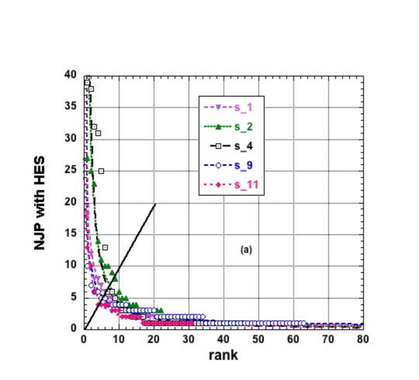
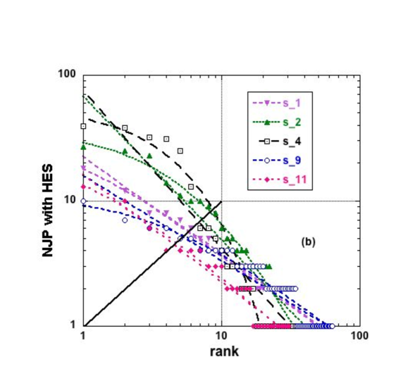
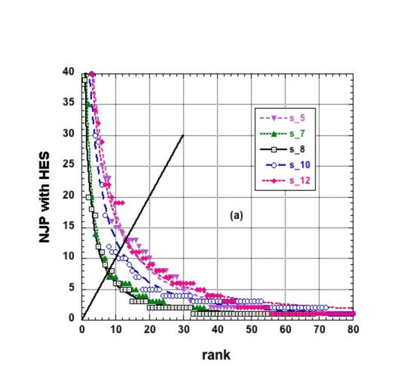
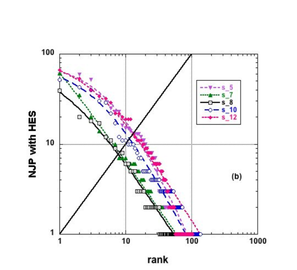
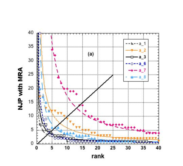
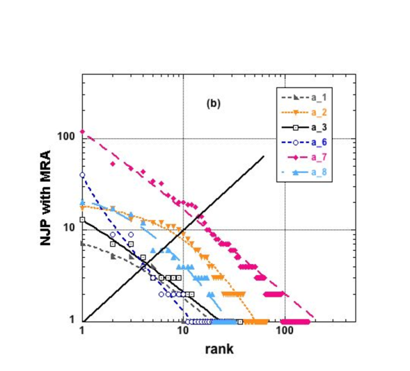
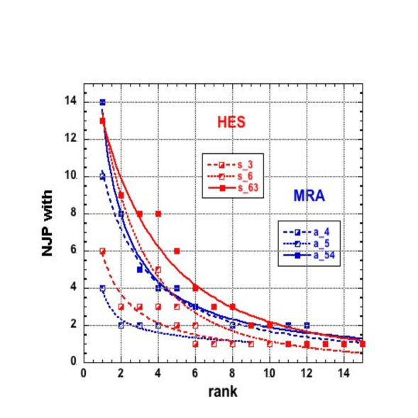
Next, observe the data when broken into sub-fields as displayed and numerically fitted on Figs. 5-8, for these two PIs. The displayed data has been grouped both according to the size of NJP and the rank range for better visibility; thus in Fig. 5, one finds the $i=$ 1, 2, 4; 9, 11 (”less prolific”) sub-fields, and in Fig. 6, the $i=$ 5, 7, 8, 10, 12 (”more prolific”) sub-fields for HES. The case of sub-fields $i=$ 4 and 5, for MRA, and of sub-fields $i=$ 3 and 6, for HES, are treated in the Appendix B, and displayed on Fig. 8, and compared to the regrouped data into $a_{54}$ and $s_{63}$.

For better visibility, the classical linear axes plots are limited to the region of interest, NJP $\leq$ 40, and NDCA $\leq$ 80 or less when convenient, i.e., where the $m_{a}$ index can be measured (Ausloos 2013), as suggested by the diagonal line indicating the core threshold. On such linear-linear axes the power law fits do not much indicate deviations. However, on the log-log plots, the ZMP fits are $ll$ obviously better reproducing the empirical data. The queen and king effects are often well seen.

It is interesting to observe that $\nu$ is negative in the $a_{6}$ and $a_{5}$ cases, and $a_{54}$, though the latter case is one of merged fields. This implies a $strong$ king effect for one CA of these sub-fields of MRA.

3.3 Remarks on the king, vice-roy, queen and harem effects

It is easily understood that the king and queen effects are at once seen on plots. Moreover, it has been observed that sometimes the low ranks contain more than one ”equivalent (in terms of NJP) CA”, thus one may propose the existence (or definition) of vice-roy(s), on one hand, and of a harem, on the other hand, effect. Numerically, this occurs respectively when

• $\nu\rightarrow$ 0, and more drastically when $\nu\leq 0$, $\rightarrow$ -1;

• when $\nu$ is large.

Concerning the queen effect, it is best measured through the ratio $\zeta/\nu$, as seen by taking the derivative of $d\;ln(J)/d\;ln(r)$, i.e.

$$\frac{dln(J)}{dln(r)}=-\frac{\zeta\;r}{\nu+r}$$ (4)

which should be $\preceq$ 0, at small $r$. The harem effect is quite obvious for DS (w) and DS (j), KK (w) and KK (j), and PVdB (all types). This is also remarkably true for the largest $\nu$ cases, i.e. $a_{2}$ (see also Fig.7), $s_{4}$ and $s_{2}$. Those large $\nu$ values indicate that both PIs have published many joint papers with a short set of CAs, - often the same ones on a large number of publications, and have thus ”many queens”. In fact, according to the sub-field definitions (Bougrine 2014), these sub-fields with many queens pertain to medical topics, for HES, and experimental work on materials, for MRA. It is understandable that a team effect, with kings and queens, are to be expected in such (transdisciplinary) domains, thereby stressing the intrinsic interest of the ZMP law, whence leading to suggest the following model.

Concerning the king and vice-roy effect, it has been discussed through a comparison of HES with HES* and MRA with MRA* in Table 3; the effect is highly remarkable for JMK (j), and PC and JM, on all types of publications: they have all a few team co-leaders. It seems that such effects are strongly constraining the fits, when $\nu\leq 0.2$..

Figure 5: Number of joint publications (NJP) for HES, with co-authors ranked by decreasing importance for his 5 ”less prolific” sub-fields $s_{i}$; (see text for $i=$ 1, 2, 4, 9, 11 definition): (a) in the vicinity of the co-author core measure; (b) log-log display of (a); best fits, i.e. power law in (a) and ZMP in (b), are given for the overall range; the co-author core can be easily deduced from the diagonal line position

Figure 6: Number of joint publications (NJP) for HES, with co-authors ranked by decreasing importance for the 5 ”most prolific” sub-fields $s_{i}$; see text for $i=$ 5, 7, 8, 10, 12 definition; (a) in the vicinity of the co-author core measure (the co-author core can be easily deduced from the diagonal line position); (b) log-log display of (a); best fits, i.e. power law in (a) and ZMP in (b), are given for the overall range

Figure 7: Number of joint publications (NJP) for MRA, with co-authors ranked by decreasing importance for 6 different sub-fields $a_{i}$; see text for $i=$ 1, …, 8 definition; (a) in the vicinity of the co-author core measure; (b) log-log scale display of (a); the co-author core can be easily deduced from the diagonal line position; the best fits, i.e. power law in (a) and ZMP in (b), are given for the overall range

Figure 8: Number of joint publications (NJP) with co-authors ranked by decreasing importance, in the case of sub-fields 4 and 5 (for MRA) and 3 and 6 (for HES), and their merging into a sub-field, i.e. $54$ and $63$ respectively; the best ZMP law fits are given

4 Model

In so doing, it seems reasonable to suggest a model of team publications, i.e. for a popular PI and his/her CAs, along the line of Mandelbrot’s model for quantitative linguistics (Mandelbrot 1960, Amati et al. 2002, Manin 2009), in fact similar to that of city formation (Madden 1956, Rosen & Resnick 1980, Glaeser 2008). Recall that Mandelbrot has first derived the Zipf’s law assuming that the optimization of the information/cost ratio is resulting from random character sequences, i.e. the ”random typing model”. Mandelbrot’s model of texts assumes that the optimal language is one where each sequence of $n$ letters is as frequent as any other (all characters are equiprobable). Thus, the probability of any given word is exponential in length. Whence, each word’s frequency rank is asymptotically given by a power law. Nevertheless, note that it has been observed that the number of distinct words of the same length in a real language, is far from being exponential in length (Manin 2009).

In fact, Mandelbrot proposed that the language is optimal if it minimizes the average ratio of production cost to information content. This leads to Eq.(2). To do so, Mandelbrot defined the information content of a word to be the Shannon entropy, i.e. the negative logarithm of the word frequency in the text or language.

In the same spirit, one can assume to derive Eq.(1), in the present case, that the choice of CAs by a PI is at first a stochastic process, - as proposed by Hsu & Huang (2009). However, as ties developed or not with the PI, either the CAs become $quasi$ happaxes, or maintain a strong tie. Moreover the CAs attract other CAs (or reject them, for whatever reason), whence organizing a CA utility network, with the PI as hub.

One can also imagine that the choice of CAs, as time and research activity progress, has some cost or utility for the PI. He/she recognizes some interest in being associated, and publishing with one or another CA, - whatever the profound reasons. Such an optimization principle allows to demonstrate how the ”optimal state” can be achieved as a result of research evolution. The $\alpha$ exponent is close to 1, as in the case of language and of city population size optimization, i.e. a desirable situation in which the forces of concentration of coworkers balance those of competition by other external teams, called ”decentralization” in city formation (Zipf 1949, Madden 1958, Glaeser 2008). In co-authorship popularity measures, as well, the exponent $\alpha$ (and $\mu$ or $\zeta$) can be interpreted as being close to 1, because of the ”same” type of balance between attraction and rejection of coworkers by the PI his/her king and queens. Thus, one considers detachment, beside preferential attachment, which by itself would lead to a much heavier tail exponent $\zeta$.

Thus, by similarity, along such a line of reasoning, consider the joint publication cost per CA to be

$$C=\sum p_{r}\;c_{r}$$ (5)

such that the ”cost of a publication” with the CA at rank $r$ is $c_{r}$, and $p_{r}$ is the normalized value of $J_{r}$, - normalization with respect to the whole histogram surface $J(r)$. Let the average information entropy per CA be also assumed to read

$$H=-\sum p_{r}\;log_{2}(p_{r}).$$ (6)

It is easy, e.g. by the Lagrange multiplier method (Manin 2009), to show that the rank-frequency distribution $p_{r}$ will minimize the cost ratio $\hat{C}\equiv C/H$ and will have a ZMP law form if one assumes the individual cost function to be

$$c_{r}=c_{0}\>log_{2}(\nu+r),$$ (7)

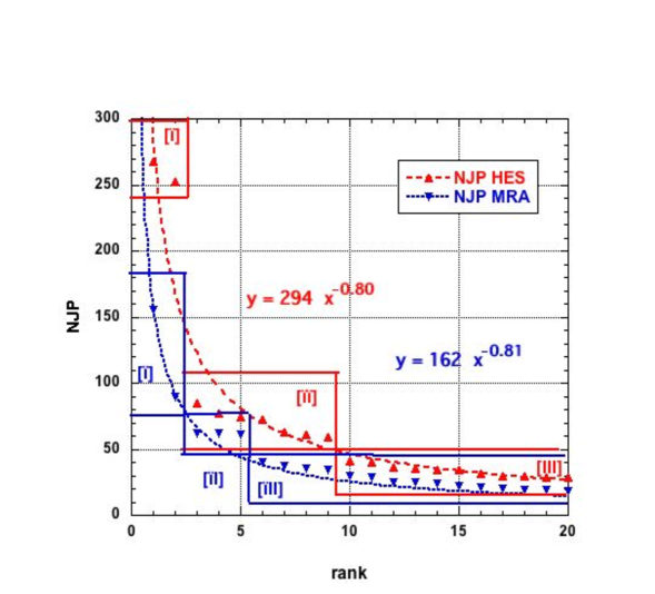
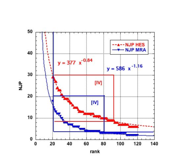
which can be negative or positive. The cost is of course high when $r$ is large. Note that if $\nu=0$, one recovers the Eq.(1) power law. Eq.(6) assumption (or ansatz) can be accepted if one considers that any research team has some hierarchical structure with a set of CA at different levels, the set increasing with the ”distance” ($\sim\;r$) from the PI. For example, the CAs can be grouped according to a visual rule, based on the behavior of $J(r)$ examined on linear or log-log plots, Fig.9. Practically, this is supplemented by trial and errors of $local$ fits in moving windows of different sizes; the groups are deduced and confirmed, choosing them from the best R² among various realistic attempts. More complicated functions (Popescu et al. 2010, Voloshynovska 2011) could be used, but a detailed parameter interpretation for such function combinations is a challenging task and requests further study, much outside this report.

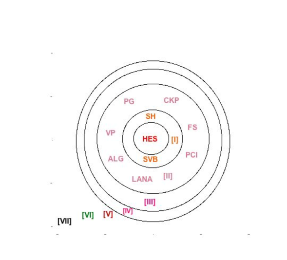
Nevertheless, the CAs can be seen as forming ”circles” around the PI, as in e.g. the HES case, Fig. 10. Note that this can be considered as the true PI community, - a visible college, since the CAs of CAs not involving the PI, have been removed from the start, by data construction. In this cluster, the PI has necessarily at least one link with some CA.

The cost of retrieving the CA at the $r$-th level can be, in a first approximation, assumed to be related to the NJP $J(r)$ of the CA, or to the rank, i.e. $log_{2}(r)$. Therefore, the parameter $\nu$ can be understood to indicate that several ”far ranked” CAs have to deal with some other ”preferred CAs” of the PI in the joint publication process.

Figure 9: Total number of joint publications (NJP) for HES and MRA, with co-authors ranked by decreasing importance allowing some vizualization of major groups of CAs; (a) for low ranks, groups I, II, and III) and (b) for group IV; the best $local$ power law fits are given as a guide to the eye

Figure 10: CAs of HES distributed in the I, II, III, and IV group according to their NJP

5 Conclusions

Most prolific scientists have joint publications on different subjects. Thus, co-authors might be specific to some research sub-field of a PI. It is thus if interest to examine, for such teams and leaders, whether the $j(r)$ relationship (Ausloos 2013) is obeyed when the research publications pertain to different sub-fields. Bougrine (2014) has broken the publication list of two such authors into sub-fields.

Observed irregularities have been thought to be due to different causes: publication inflation, proceedings counting, co-authorship inflation, and/or promotion of team size visibility. Other ”intrinsic causes” might have arisen from the large productivity of the group based on a high turnover of young researchers, with $r>>1$, as well as a steady contribution from stable partners, with $r\simeq 1$.

Here, deviations have been searched through sub-field considerations. By using the Zip-Mandelbrot-Pareto function for the distribution $J(r)$, thus having one more parameter ($\nu)$, it has been observed that the statistics on one hand is much improved. On the other hand, the introduction of the extra parameter, and the observation of its range of values, has suggested a model based on a co-author cost scheme, similar to the models of language usage and city population size distributions. One must admit that the model is a rather common sense model to anyone having worked with co-authors, in large or small teams.

However, the analysis has indicated the sensitivity of the sub-field notion, on one hand, and of the co-author distribution, on the other hand. Moreover the notion of cost and utility of co-authorship are introduced, but demand further elaboration; some work will be useful along such lines, for better quantification also.

Notice that the cost can be positive or negative according to the value of $\nu$; see Eq. (7). This observation can be considered to be already useful in order to imagine that one can be introducing selection and rewarding policies in the career of members of teams, along the co-author core measure. Technically, one could thus measure the relevant strength of a research group centered on some leader by combining the $h$-index and the $m_{a}$ measure in a three dimensional ($J$, $q$, $r$) space taking into account the quotations $q$ of co-authored papers.

Acknowledgements Thanks to J. Miskiewicz and H. Bougrine for private communications on their respective work, comments prior to manuscript submission and making available the relevant publication list data mentioned in the text. I warmly thank all colleagues who have kindly provided relevant data. This paper is part of scientific activities in COST Action TD1210.

	4 param. ZMP, Eq.(3)			3 param. ZMP, Eq.(2)
NJP	$\eta$	$\lambda$	$c$	$\nu$	$b$	$\mu\equiv\zeta$	R2
HES (w)	0.177	0.376	165.9	0.10	335.0	0.835	0.916
HES∗ (w)	1.741	0.236	230.6	7.384	1128.0	1.098	0.987
MRA (w)	0.523	0.558	161.7	0.876	276.25	0.975	0.988
MRA∗ (w)	1.547	0.266	206.7	4.149	723.3	1.203	0.988

Table 3: Summary of fit parameters to NJP data corresponding to Fig.1; the parameters correspond to the various formulae discussed in the text, Eqs.(2)-(3); HES^∗ and MRA^∗ indicate that the two lowest rank data points corresponding to a strong king and vice-roy effect have been removed before fit attempts; the regression fit coefficient R² is given for the different cases; data has been rounded up to significant decimals

	4 param. ZMP, Eq.(3)
NJP	$\eta$	$\lambda$	$c$	$\mu$	R2
$s_{1}$	2.957	4.442	96.058	0.838	0.988
$s_{2}$	1.715	0.181	134.08	2.074	0.978
$s_{4}$	1.176	0.021	503.44	$q.pw.t$	0.940
$s_{9}$	246.4	64.59	1262.5	0.859	0.961
$s_{11}$	2.989	3.126	79.342	0.989	0.974
$s_{5}$	1.401	0.188	144.63	$1.68$	0.979
$s_{7}$	0.257	1.308	98.392	1.054	0.994
$s_{8}$	1.346	1.148	105.54	1.128	0.982
$s_{10}$	1.227	0.291	99.365	1.427	0.982
$s_{12}$	1.527	0.264	154.89	$1.19$	0.987
$a_{1}$	1.668	0.644	17.642	1.088	0.939
$a_{2}$	2.048	0.058	241.0	$q.pw.t$	0.980
$a_{3}$	1.868	5.118	73.331	0.893	0.971
$a_{6}$	-2.013	2.769	31.154	1.199	0.988
$a_{7}$	0.219	0.797	117.1	0.925	0.981
$a_{8}$	1.96	0.292	113.9	1.852	0.971
$s_{3}$	0.734	1.098	10.69	0.989	0.911
$s_{6}$	0.964	$exp.t$	15.39	$exp.t$	$0.970$
$s_{63}$	1.016	0.056	17.68	$exp.t$	$0.970$
$a_{4}$	2.137	0.851	49.00	1.427	0.969
$a_{5}$	-2.963	4.991	5.374	0.425	0.895
$a_{54}$	-0.075	3.479	39.44	0.844	0.989

Table 4: Summary of fit parameters to NJP data grouped as for Figs. 5-8, according to different sub-fields of HES ($s_{i}$) and MRA ($a_{i}$); the fit parameter values correspond to the 4-ZMP form, Eq. (3); $q.pw.t$ indicates the presence of both a strong queen and power law tail effect, while $exp.t$ indicates a strong exponential tail cut-off, i.e. cases for which the scaling parameters have large error bars; the regression fit coefficient R² is given for the different cases; data has been rounded up to significant decimals; error bars $\leq$ 10%

Appendix A. ZMP fits with 3 or 4 free parameters

Using the 3-parameter free ZMP function, Eq.(3), for data fitting is much more troublesome than fitting with the Zipf hyperbolic law (Fairthorne 1969, Haitun 1982, Iszak 2006). Thus, a variant of the ZMP law, i.e. the 4-parameter relation Eq.(3) is sometimes proposed, since it allows for one more scaling parameter. It is often observed that the 4-ZMP has some advantage with respect to the 3-ZMP, from the point of view of the stability of the solutions of the non linear system of equations for the fit parameters. This is interpreted as due to the fact that the numerical values of the other parameters ($\mu$, $\eta$, $\lambda$, and the more so $c$) fall into more compact ranges. For examples, compare the amplitudes $c$ and $b$ for $s_{2}$ and $s_{4}$, respectively, in Tables 2 and Table 4 for the 4-ZMP and 3-ZMP fits.

However nothing drastic has been found in the present cases, as seen from Tables 3-5. Moreover, the meaning of $\nu$, in the 3-ZMP case seems more easily interpretable than the $\eta$ and $\lambda$ values in the 4-ZMP.

It should be emphasized that the R² values are identical, up to the third decimal, for the 3- and 4-ZMP parameter law fits, see Table 4, except for $s_{6}$ and subsequently $s_{63}$, nevertheless found close to each other, as likely due to an $exp.t$ behavior pointing to a strong exponential tail cut-off, - in which cases the empirical laws can be hardly expected to hold. Thus, it is observed that $\mu\equiv\zeta$ in all cases, - i.e. the relevant conclusion.

Appendix B. On merging sub-fields

In order to investigate the effect of reduced size of data in considering sub-fields, Bougrine (2014) merged 2 sub-fields into a single one, both in the case of MRA and HES. For comparison, and completeness, ZMP and power law fits have been made on $a_{4}$ and $a_{5}$ merged into $a_{54}$ on one hand, and on $s_{3}$ and $s_{6}$ merged into $s_{65}$ on the other hand. The parameters resulting from the fits are given in Table 2. The fits are displayed in Fig. 8. In such cases, with not many data points, the co-author core is low, and the effect of many CAs at rank $r\geq 4$ or 6 respectively is rather important. Thus, the instability of the fits with respect to initial conditions is due to the presence of a strong exponential cut-off superposed on the power law tail.

These features indicate the sensitivity of the sub-field definition, on one hand, and of the co-author distribution, on the other hand.

	4 param. ZMP				3 param. ZMP					power law
CDF	$\eta$	$\lambda$	$c$		$\nu$	$b$	$\mu\equiv\zeta$	R2		$a$	$\alpha$	R2
$a_{2}$	1.117	0.735	1.154		1.515	1.626	1.120	0.970		0.603	0.943	0.960
$a_{7}$	7.127	4.408	7.759		1.597	1.584	1.143	0.996		0.898	1.032	0.932

Table 5: Summary of fit parameter values to $a_{2}$ and $a_{7}$ frequency-size cumulative distribution function (CDF) data with notations explained in the text, - corresponding to Figs. 6 and 7??? respectively; the parameters correspond to the various formulae discussed in the text, Eqs.(1)-(3); the regression fit coefficient R² is given for the different cases

Figure 11: Log-log scale display of the number of joint publications (NJP) on magnetic materials, for MRA, with co-authors, ranked by decreasing importance, and of the corresponding frequency-size cumulative distribution function (CDF); best fits, over the whole data range are shown for the power law and ZMP law

Figure 12: Log-log scale display of the number of joint publications (NJP) on superconductivity, for MRA, with co-authors, ranked by decreasing importance, and of the corresponding frequency-size cumulative distribution function (CDF); best fits, over the whole data range are shown for the power law and ZMP law

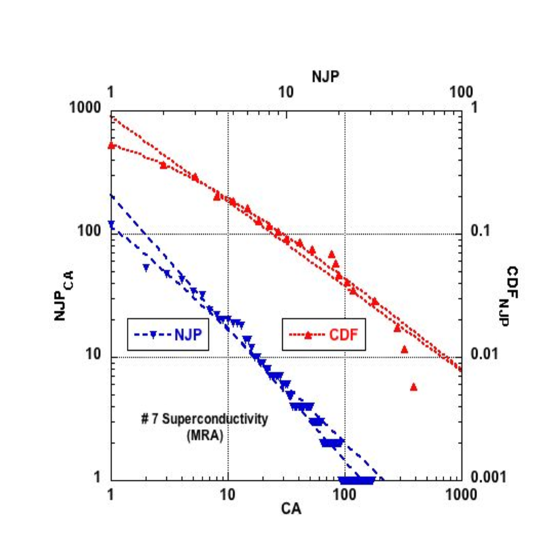
Appendix C. On cumulative distribution functions (CDF)

In Informetrics, one prefers to fit empirical data to some size-frequency functional form using a maximum likelihood fit, rather than making a least squares fit for the rank-frequency distribution. Indeed, one can also ask, as did Pareto (1896), how many times one can find an ”event” greater than some size $y$, i.e. study the size-frequency relationship. Pareto found out that the cumulative distribution function (CDF) of such events follows an inverse power of $y$, or in other words, $P\;[Y>y]\sim y^{-\kappa}$. Thus, the (number or) frequency $f$ of such events of size $y$, (also) follows an inverse power of $y$.

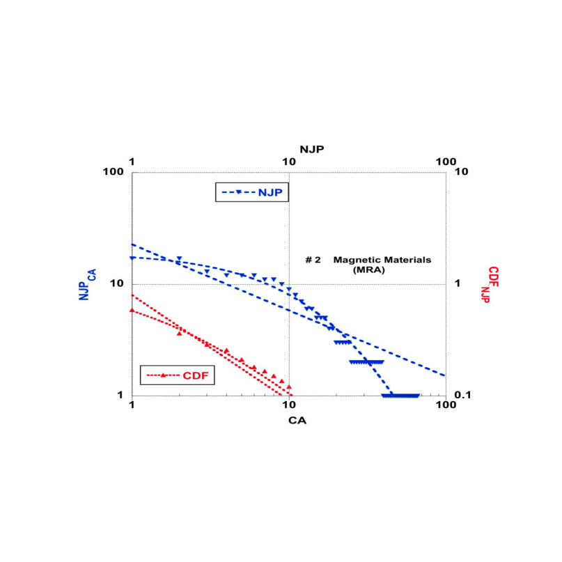
Thus, for illustration, ZMP and power law fits have been made on two of MRA major sub-fields, i.e. $a_{2}$ and $a_{7}$. A log-log scale display of the number of joint publications (NJP) with co-authors ranked by decreasing importance and the corresponding CDF are shown in Figs. 11-12. Both the power law and ZMP law fits are shown for the all $r$ range. Note that the NJP data and fits are those seen in Fig. 7, with numerical values in Table 1.

The ”queen effect” is well seen on the NJP data and fits, on Fig. 11, but not so much on the CDF. The ”king effect” is well seen on the NJP data and fits, on Fig. 12, but the CDF shows a pronounced cut-off at high $r$. Therefore it would seem that the CDF is less pertinent to observe minute effects. This is understandable since the CDF results from an integration scheme. However, again understandably, the CDF fits are much more stable.

References

Amati, G. & van Rijsbergen, C. J. (2002). Term frequency normalization via Pareto distributions. Advances in Information Retrieval, F. Crestani, M. Girolami, C.J. van Rijsbergen (Eds.), LNCS 2294, pp. 183–192.

Ausloos, M. (2013). A scientometrics law about co-authors and their ranking. The co-author. Scientometrics, 95(3), 895-909.

Ausloos, M. (2014). Binary Scientific Star Coauthors Core Size. Scientometrics, in press

Bar-Ilan, J. (2008). Which h-index? - A comparison of WoS, Scopus and Google Scholar. Scientometrics, 74(2), 257-271.

Benguigui, L. & Blumenfeld-Lieberthal, E. (2011). The end of a paradigm is Zipf’s law universal?. Journal of Geographical Systems, 13(2), 87-100.

Bonitz, M., & Scharnhorst, A., (2011). Competition in science and the Matthew core journals. Scientometrics, 51(1), 37–54.

Bonitz, M., Bruckner, E., & Scharnhorst, A., (1999). The Matthew index-concentration patterns and Matthew core journals. Scientometrics, 44(3), 361-378.

Bornmann, L., Mutz, R., & Daniel, H. (2008). Are there better indices for evaluation purposes than the h-index? A comparison of nine different variants of the h-index using data from biomedicine. Journal of the American Society for Information Science and Technology, 59(5), 830-837.

Bougrine, H. (2014). Subfield Effects on the Core of Coauthors. Scientometrics, 98(2), 1047-1064.

Cole, J.R. & Cole, S. (1972). The Ortega Hypothesis Citation analysis suggest that only a few scientists contribute to scientific progress. Science, 178(4059), 368–375.

Egghe, L. (2005). Power Laws in the Information Production Process Lotkaian Informetrics. Amsterdam: Elsevier

Egghe, L., & Rousseau, R. (1990). Introduction to Informetrics. Quantitative Methods in Library, Documentation and Information Science. Amsterdam: Elsevier

Fairthorne, R.A. (1969). Empirical hyperbolic distributions (Bradford-Zipf-Mandelbrot) for bibliometric description and prediction. Journal of Documentation, 25(4), 319-343.

Garfield, E. (2006). Citation indexes for science. A new dimension in documentation through association of ideas. International journal of epidemiology, 35(5), 1123–1127.

Glaeser, E.L. (2008). Cities, agglomeration and spatial equilibrium. New York: Oxford University Press

Haitun, S. D. (1982). Stationary scientometric distributions. Part. 1. Different approximations. Scientometrics, 4(1), 5-25.

Hirsch, J. E. (2005). An index to quantify an individual’s scientific research output. Proceedings of the National Academy of Sciences USA, 102(46), 16569-16572.

Hirsch, J. E. (2010). An index to quantify an individual’s scientific research output that takes into account the effect of multiple co-authorship. Scientometrics, 85(3), 741-754.

Hsu, J. W. & Huang, D. W. (2009). Distribution for the number of co-authors. Physical Review E, 80(5), 057101.

Iszak, J. (2006). Some practical aspects of fitting and testing the Zipf-Mandelbrot model. Scientometrics, 67(1), 107–120.

Jarque, C. M., & Bera, A. K. (1980). Efficient tests for normality, homoscedasticity and serial independence of regression residuals. Economics Letters 6(3), 255-259.

Jefferson, M. (1939) The law of primate city. Geographical Review, 29(2), 226-232.

Laherrère, J. & Sornette, D. (1998). Stretched exponential distributions in nature and economy fat tails with characteristic scales. European Physics Journal B, 2(4), 525-539.

Madden C.H. (1958). Some Temporal Aspects of the Growth of Cities in the United States. Economic Development and Cultural Change, 6(2), 143-170.

Mandelbrot, B. (1960). The Pareto-Levy Law and the Distribution of Income. International Economics Review, 1(2), 79-106.

Manin, D. Yu. (2009). Mandelbrot’s Model for Zipf’s Law Can Mandelbrot’s Model Explain Zipf’s Law for Language?. Journal of Quantitative Linguistics, 16(3), 274–285.

Miskiewicz, J. (2013). Effects of Publications in Proceedings on the Measure of the Core Size of Coauthors. Physica A, 392(20), 5119-5131.

Newman, M.E.J. (2001). The structure of scientific collaboration networks. Proceedings of the National Academy of Sciences USA, 98(2), 404-409.

Pareto, V. (1896) Cours d’Economie Politique. Geneva, Switzerland: Droz.

Popescu, I. I., Altmann, G., Köhler, R. (2010). Zip’s law - another view. Quality and Quantity, 44(4), 713-731.

Price, D. J. de S. (1956). The exponential curve of science. Discovery, 17(6), 240-243.

Rosen, K.T & Resnick, M. (1980). The size distribution of cities an examination of the Pareto law and primacy. Journal of Urban Economics, 8(2), 165–186.

Rousseau, R. (2006). New developments related to the Hirsch index. Science Focus, 1(1), 23-25.

Schreiber, M. (2010). Twenty Hirsch index variants and other indicators giving more or less preference to highly cited papers. Annalen der Physik (Berlin), 522(8), 536-554.

Tsallis, C., & Albuquerque, M.P. (2000). Are citations of scientific papers a case of nonextensivity?. European Physics Journal B, 13(4), 777-780.

van Raan, A. F. J. (1996), Advanced bibliometric methods as quantitative core of peer review based evaluation and foresight exercises. Scientometrics, 36(3), 397-420.

Voloshynovska, I. A. (2011) Characteristic Features of Rank-Probability Word Distribution in Scientific and Belletristic Literature. Journal of Quantitative Linguistics, 18(3), 274-289.

West, B.J. & Deering, B. (1995) The Lure of Modern Science Fractal Thinking. Singapore: World Scient.

Zipf, G.K. (1949). Human Behavior and the Principle of Least Effort An Introduction to Human Ecology. Cambridge: Addison Wesley.