Powerful nonparametric checks for quantile regression

Abstract

We address the issue of lack-of-fit testing for a parametric quantile regression. We propose a simple test that involves one-dimensional kernel smoothing, so that the rate at which it detects local alternatives is independent of the number of covariates. The test has asymptotically gaussian critical values, and wild bootstrap can be applied to obtain more accurate ones in small samples. Our procedure appears to be competitive with existing ones in simulations. We illustrate the usefulness of our test on birthweight data.

Keywords: Quantile regression, Omnibus test, Smoothing.

MSC2000: Primary 62G10

1 Introduction

Quantile regression, as introduced by Koenker and Bassett (1978), has emerged as an alternative to mean regression. It allows for a richer data analysis by exploring the effect of covariates at different quantiles of the conditional distribution of the variable of interest. Parametric quantile regression generalizes usual regression are is particularly valuable if variables have asymmetric distributions or heavy tails. Koenker’s monograph (2005) and the review of Yu et al. (2003) detail the theory and practice of quantile regression.

As in any statistical modeling exercice, it is crucial to check the fit of a parametric quantile model. There has been a large effort devoted to testing of the fit of parametric mean regressions, however only few lack-of-fit tests of parametric quantile regressions. He and Zhu (2003) extend the approach of Stute (1997) and is based on a vector-weighted cumulative summed process of the residuals. Bierens and Ginther (2002) generalize the integrated conditional moment test of Bierens and Ploberger (1997) to quantile regression. In both cases, the limit distribution of the test statistic is a non-linear functional of a Gaussian process, so that implementation may require rather involved computations to obtain critical values. Zheng (1998) use kernel smoothing over the design space, to obtain an asymptotically pivotal test statistic. Horowitz and Spokoiny (2002) extend such an approach and propose an adaptive procedure to choose the smoothing parameter. As in any multidimensional nonparametric problem, the curse of dimensionality may be detrimental to the performances of the test, see e.g. Lavergne and Patilea (2012) for illustrations.

In this paper, we introduce a new testing methodology that avoids multidimensional smoothing, but still yield an omnibus test. Our test has three specific features. First, it does not require smoothing with respect to all covariates under test. This allows to mitigate the curse of dimensionality that appears with nonparametric smoothing, hence improving the power properties of the test. Second, the test statistic is asymptotically pivotal, while wild bootstrap can be used to obtain small samples critical values of the test. This yields a test whose level is well controlled by bootstrapping, as shown in simulations. Third, our test equally applies whether some of the covariates are discrete.

The paper is organized as follows. In Section 2, we present our testing procedure, we study its asymptotic behavior under the null hypothesis and under a sequence of local alternatives, and we establish the validity of wild bootstrap. In Section 3, we compare the small sample behavior of our test to some existing procedures, and we illustrate its use on birthweight data. Section 3 concludes. Section 4 gathers our technical proofs.

2 Lack-of-Fit Test for Quantile Regression

2.1 Principle and Test

Consider modeling the quantile of a real random variable $Y$ conditional upon covariates $Z\in\mathbb{R}^{q}$, $q\geq 1$. We assume that $Z=(W,X^{\prime})^{\prime}$, where $W$ is continuous and admits a density with respect to the Lebesgue measure, while $X$ may include both continuous and discrete variables. Formally, if $F(\cdot\mid z)$ denotes the conditional distribution of $Y$ given $Z=z$, the $\tau$-th conditional quantile is $Q_{\tau}(z)=\inf\{y:F(y\mid z)\geq\tau\}$. Assuming $F(\cdot\mid z)$ is absolutely continuous for almost all $z$, this is equivalent to $F(Q_{\tau}(z)\mid z)=\tau$. The parametric quantile regression model of interest posits that the conditional $\tau$-th quantile of $Y$ is given by $g(Z;\beta_{0})$, where $g(\cdot;\beta)$ is known up to the parameter vector $\beta\in B\subset\mathbb{R}^{p}$, that is,

$$Y=g(Z;\beta_{0})+\varepsilon,\qquad F\left(g(Z;\beta_{0})\mid Z\right)=\tau\,.$$ (2.1)

The validity of our parametric quantile regression is thus equivalent to

$${H}_{0}:\ \exists\,\beta_{0}\in B\ :\ F(g(Z;\beta_{0})\mid Z)-\tau=\mathbb{E}\left\{\mathbb{I}\{Y\leq g(Z;\beta_{0})\}-\tau\mid Z\right\}=0\,\text{a.s.}$$ (2.2)

Hence testing the the correct specification of our parametric quantile regression models reduces to testing a zero conditional mean hypothesis. The alternative hypothesis is then

$${H}_{1}:\ \mathbb{P}\left[\mathbb{E}\left\{\mathbb{I}\{Y\leq g(Z;\beta)\}-\tau\mid Z\right\}=0\right]<1\quad\text{for any }\beta\in B\,.$$

The key element of our testing approach is the following lemma. See also Lavergne et al. (2014) for a related result. First let us introduce some notation. Hereafter, if $g:\mathbb{R}^{k}\rightarrow\mathbb{R}$ is an integrable function, $\mathcal{F}[g]$ denotes its Fourier transform, that is

$$\mathcal{F}[g](t)=\int_{\mathbb{R}^{k}}\exp(-2\pi it^{\prime}u)g(u)du\,.$$

Lemma 2.1

Let $\left(W_{1},\,X_{1},\,U_{1}\right)$ and $\left(W_{2},\,X_{2},\,U_{2}\right)$ be two independent draws of $\left(W,\,X,\,u\right)$, and $K(\cdot)$ and $\psi(\cdot)$ even functions with (almost everywhere) positive Fourier integrable transforms. Define

$$I\left(h\right)=\mathbb{E}\left[U_{1}U_{2}h^{-p}K\left(\left(W_{1}-W_{2}\right)/h\right)\psi\left(X_{1}-X_{2}\right)\right]\,.$$

Then for any $h>0$, $\mathbb{E}\left[U\mid W,X\right]=0\,\;a.s.\Leftrightarrow I(h)=0$.

Proof.Let $\langle\cdot,\cdot\rangle$ denote the standard inner product and $\mathcal{F}\left[K\right]$ be the Fourier transform of $K(\cdot)$. Using Fourier Inversion Theorem, change of variables, and elementary properties of conditional expectation,

$$I(h) = \mathbb{E}\left[U_{1}U_{2}\int_{\mathbb{R}^{p}}e^{2\pi i\langle t,\;W_{1}-W_{2}\rangle}\mathcal{F}\left[K\right]\left(th\right)dt\int_{\mathbb{R}^{q}}e^{2\pi i\langle s,\;X_{1}-X_{2}\rangle}\mathcal{F}\left[\psi\right]\left(s\right)ds\right]$$

$$= \int_{\mathbb{R}^{q}}\int_{\mathbb{R}^{p}}\left|\mathbb{E}\left[\mathbb{E}\left[U\mid W,X\right]e^{2\pi i\left\{\langle t,W\rangle+\langle s,X\rangle\right\}}\right]\right|^{2}\mathcal{F}\left[K\right]\left(th\right)\mathcal{F}\left[\psi\right]\left(s\right)dtds\,.$$

Since the Fourier transforms $\mathcal{F}\left[K\right]$ and $\mathcal{F}\left[\psi\right]$ are strictly positive, $I(h)=0$ iff

$$\mathbb{E}\left[\mathbb{E}\left[U\mid W,X\right]e^{2\pi i\left\{\langle t,W\rangle+\langle s,X\rangle\right\}}\right]=0\quad\forall t,s\Leftrightarrow\mathbb{E}\left[U\mid W,X\right]=0\qquad\mbox{a.s.}\qquad\rule{5.0pt}{5.0pt}$$

From the above results, it is sufficient to test whether $I(h)=0$ for any arbitrary $h$. We chose to consider a sequence of $h$ decreasing to zero when the sample size increases, which is one of the ingredient that allows to obtain a tractable asymptotic distribution for the test statistic. Assume we have at hand a random sample $(Y_{i},W_{i},X_{i})$, $1\leq i\leq n$, from $(Y,W,X)$. Then we can estimate $I\left(h\right)$ by the second-order U-statistic

$$I_{n}\left(\beta_{0}\right)=I_{n}\left(\beta_{0};h\right)=\frac{1}{n(n-1)}\sum\limits_{1\leq j\neq i\leq n}U_{i}\left(\beta_{0}\right)U_{j}\left(\beta_{0}\right)\frac{1}{h}K_{h}\left(W_{i}-W_{j}\right)\psi(X_{i}-X_{j})$$

where $U_{i}(\beta)=\mathbb{I}\{Y_{i}\leq g(Z_{i};\beta)\}-\tau$ and $K_{h}(\cdot)=K(\cdot/h)$.

For estimating $\beta_{0}$, we follow Koenker and Bassett (1978), who showed that under (2.1) a consistent estimator of $\beta_{0}$ is obtained by minimizing

$$\arg\min_{\beta}\sum_{i=1}^{n}\rho_{\tau}\left(Y_{i}-g(Z_{i};\beta)\right)\,,$$ (2.3)

where $\rho_{\tau}(e)=\left(\tau-\mathbb{I}(e<0)\right)\,e$ is the so-called check function. While this is not a differentiable optimization problem, it is convex and tractable, see e.g. Koenker (2005) for some computational algorithms. Let us define

$$T_{n}=nh^{1/2}\frac{I_{n}(\widehat{\beta})}{v_{n}}\quad\mbox{where }\quad v_{n}^{2}=\frac{2\,\tau^{2}(1-\tau)^{2}}{n(n-1)}\sum\limits_{j\neq i}h^{-1}K_{h}^{2}\left(W_{i}-W_{j}\right)\psi^{2}(X_{i}-X_{j})\;.$$ (2.4)

An asymptotic $\alpha$-level test of ${H}_{0}$ is then

Reject $H_{0}$ if $T_{n}\geq z_{\alpha}$, where $z_{\alpha}$ is the $(1-\alpha)-$quantile of the standard normal distribution.

Our test statistic is very similar to the one proposed by Zheng (1998), but the latter uses smoothing on all components of $Z$ while we smooth only on the first component $W$.

The statistic $v_{n}^{2}$ is the variance of $nh^{1/2}I_{n}(\beta_{0})$ conditional on the $Z_{i}$ under ${H}_{0}$. In general, $v_{n}^{2}$ does not consistently estimate the conditional variance of $nh^{1/2}I_{n}(\beta)$ under the alternative hypothesis. In some cases $v_{n}^{2}$ overestimates this conditional variance (this is certainly the case for misspecified median regression model because $\tau(1-\tau)$ attains the maximum value at $\tau=1/2$), so that the test may suffer some power loss. In a mean regression context, Horowitz and Spokoiny (2001) and Guerre and Lavergne (2005) proposed to use a nonparametric estimator of the conditional variance. This might be adapted to quantile regression, but in simulations our test appears to be well-behaved and more powerful than competitors, so we decided in favor of the simplest estimator $v_{n}^{2}$.

2.2 Behavior Under the Null Hypothesis

To derive the asymptotic properties of our lack-of-fit test, we introduce our set of assumptions on the data-generating process, the parametric model (2.1), the functions $K(\cdot)$ and $\psi(\cdot)$, and the bandwidth $h$.

Assumption 2.1

(a) The random vectors $(\varepsilon_{1},Z_{1}^{\prime})^{\prime},\ldots,(\varepsilon_{n},Z_{n}^{\prime})^{\prime}$ are independent copies of the random vector $(\varepsilon,Z^{\prime})^{\prime}\in\mathbb{R}^{1+q}$. The conditional $\tau$th quantile of $\varepsilon$ given $Z=\left(W,X^{\prime}\right)^{\prime}$ is equal to zero.

(b) The variable $W$ admits an absolutely continuous density with the respect of the Lebesgue measure on the real line.

(c) The conditional density $f_{\varepsilon}(\cdot\mid z)$ of $\varepsilon$ given $Z=z$ is uniformly bounded. There exists $a>0$ such that $f_{\varepsilon}(\cdot\mid z)$ is differentiable on $(-a,a)$ for any $z$ with $\left|f_{\varepsilon}^{\,\prime}(0\mid z)\right|\leq C\infty$. Moreover, the derivatives $f_{\varepsilon}^{\,\prime}(\cdot\mid z)$ satisfy a uniform Hölder continuity condition, that is there exist positive constants $C_{2}$ and $c$ independent of $z$ such that $\forall\left|u_{1}\right|,\left|u_{2}\right|\leq a$, $\left|f_{\varepsilon}^{\,\prime}(u_{1}\mid z)-f_{\varepsilon}^{\,\prime}(u_{2}\mid z)\right|\leq C_{2}\left|u_{1}-u_{2}\right|^{c}$.

Assumption 2.2

(a) The parameter space $B$ is a compact convex subset of $\mathbb{R}^{p}$. $\beta_{0}$ is the unique solution of $\min_{B}\mathbb{E}\left[\rho_{\tau}\left(Y-g(Z,\beta)\right)\right]$ and is an interior point of $B$.

(b) The matrix

$$\mathbb{E}\left[f_{\varepsilon}(0\mid Z\,)\frac{\partial}{\partial\beta}{g}(Z;\beta_{0})\frac{\partial}{\partial\beta^{\prime}}{g}^{\prime}(Z;\beta_{0})\right]$$

is finite and nonsingular.

(c) There exists functions $A\left(\cdot\right)$, $B\left(\cdot\right)$, and $D\left(\cdot\right)$, with $\mathbb{E}[A^{4}(\,Z\,)]$, $\mathbb{E}[B^{2}(\,Z\,)]<\infty$, and $\mathbb{E}[D^{4}(\,Z\,)]$, such that

$$\left\|\frac{\partial}{\partial\beta}{g}(z;\beta)\right\|\leq A\left(z\right),\qquad\left\|\frac{\partial}{\partial\beta}{g}(z;\beta)\frac{\partial}{\partial\beta^{\prime}}{g}^{\prime}(z;\beta)\right\|\leq D(z)\qquad\text{for any }\beta\,,$$

$$\left\|\frac{\partial}{\partial\beta}{g}(z;\beta_{1})-\frac{\partial}{\partial\beta}{g}(z;\beta_{2})\right\|\leq B(z)\left\|\beta_{1}-\beta_{2}\right\|\qquad\text{for any }z,\beta_{1},\beta_{2}\,.$$

(d) The class of functions $\{g(Z;\beta):\beta\in B\}$ is a Vapnik-Červonenkis (VC) class.

Assumption 2.3

(a) The function $K(\cdot)$ is a bounded symmetric univariate density of bounded variation with positive Fourier transform.

(b) The function $\psi(\cdot)$ is a bounded symmetric multivariate function with positive Fourier transform.

(c) $h\rightarrow 0$ and $n^{\alpha}h^{2}\rightarrow\infty$ for some $\alpha\in(0,1)$ as $n\rightarrow\infty$.

Our assumptions combine standard assumptions for parametric quantile regression estimation and specific ones for our lack-of-fit test. Among the latter, the conditions on the error term $\varepsilon$ impose neither independence of $\varepsilon$ and $Z$, nor a specific form of dependence such as $\varepsilon=s\left(Z\right)e$ with $e$ independent of $Z$ as in He and Zhu (2003). Assumption 2.2(d) is a mild technical condition that guarantees suitable uniform rates of convergence for some $U-$processes appearing in the proofs. This condition is satisfied for many parametric models, for instance when $g(Z,\beta)=q(Z^{\prime}\beta)$ with $q:\mathbb{R}\rightarrow\mathbb{R}$ monotone or of bounded variation, see e.g. van der Vaart and Wellner (1996, Section 2.6). Also, if there is $\beta\in B$ such that $g(Z,\beta)$ is squared integrable, then Assumption 2.2(d) follows from 2.2(c). Assumptions on $K(\cdot)$ allows for the use of a triangular, normal, logistic, Student (including Cauchy), or Laplace densities. For $\psi(\cdot)$, one can choose e.g. $\psi(x)=\exp(-\|x\|^{2})$, or any multivariate extension of the aforementioned densities. Restrictions on the bandwidth are compatible with optimal choices for regression estimation, see e.g. Härdle and Marron (1985), and for regression checks, see Guerre and Lavergne (2002) and Horowitz and Spokoiny (2002). The following theorem states the asymptotic validity of our test.

Theorem 2.2

Under the Assumptions 2.1 to 2.3, the test based on $T_{n}$ has asymptotic level $\alpha$ under $H_{0}$.

2.3 Behavior under Local Alternatives

We now investigate the behavior of our test when $H_{0}$ does not hold, and specifically we consider a sequence of local alternatives of the form

$${H}_{1n}:\ Y=g(Z;\beta_{0})+r_{n}\delta(Z)+\varepsilon,\qquad F\left(g(Z;\beta_{0})\mid Z\right)=\tau\,,$$ (2.5)

where $r_{n}$, $n\geq 1$, is a sequence of real numbers tending to zero and $\delta(Z)$ is a real-valued function satisfying

$$\mathbb{E}\left[f_{\varepsilon}(0\mid Z\,)\delta(Z)\frac{\partial}{\partial\beta}{g}(Z;\beta_{0})\right]=0\quad\mbox{\rm and }\quad 0<\mathbb{E}[\delta^{4}(Z)]<\infty\,.$$ (2.6)

This condition ensures that our sequence of models (2.5) does not belong to the null hypothesis $H_{0}$. We do not impose any smoothness restriction on the function $\delta(\cdot)$ as is frequent in this kind of analysis, see e.g. Zheng (1998). As shown in Lemma 4.1 in the Proofs section, $\widehat{\beta}-\beta_{0}=O_{\mathbb{P}}(n^{-1/2}+r_{n}^{2})$ under ${H}_{1n}$. Our next result states that these local alternatives can be detected whenever $r_{n}^{2}nh^{1/2}\rightarrow\infty$. Hence our test does not suffer from the curse of dimensionality against local alternatives, since its power is unaffected by the number of regressors.

Theorem 2.3

Under Assumptions 2.1 to 2.3, the test based on $T_{n}$ is consistent against the sequence of alternatives ${H}_{1n}$ with $\delta(Z)$ satisfying (2.6) if $r_{n}^{2}nh^{1/2}\rightarrow\infty$.

2.4 Bootstrap Critical Values

The asymptotic approximation of the behavior of $T_{n}$ may not be satisfactory in small samples as is customary in smoothing-based lack-of-fit tests. This motivates the use of bootstrapping for obtaining critical values. The distribution of $T_{n}$ depends weakly on the distribution of the error term $\varepsilon$, because $\mathbb{I}\{Y\leq g(Z;\beta_{0})\}-\tau$ under $H_{0}$ is a Bernouilli random variable irrespective of the particular distribution of $\varepsilon$. The same phenomenon is noted by Horowitz and Spokoiny (2002) for their test statistic. Their proposal is thus to naively (or nonparametrically) bootstrap from the empirical distribution of the residuals. This is a valid bootstrap procedure when errors are identically distributed, and it remains asymptotically valid for non identically distributed errors. A first possibility is thus to adopt naive residual bootstrap for our test. Alternatively, He and Zhu (2003) note that one could use any continuous distribution with the $\tau$-th quantile equal to 0. This constitutes a second possibility. While asymptotically valid, these two methods do not account for potential heteroscedastic errors. Thus a third possibility is the wild bootstrap method for quantile regression introduced by Feng et al. (2011). The wild bootstrap procedure for our test works as follows.

1. Let $\widehat{\varepsilon}_{i}=Y_{i}-g(Z_{i};\widehat{\beta})$, $1\leq i\leq n$, and $w_{1},\cdots w_{n}$ be bootstrap weights generated independently from a two-point mass distribution with probabilities $1-\tau$ and $\tau$ at $2(1-\tau)$ and $-2\tau$. Compute $\varepsilon_{i}^{\ast}=w_{i}|\widehat{\varepsilon}_{i}|$ and $Y_{i}^{\ast}=g(Z_{i};\widehat{\beta})+\varepsilon_{i}^{\ast}$ for each $i=1,...,n$.

2. Use the bootstrap data set $\left\{Y_{i}^{\ast},Z_{i}:i=1,...,n\right\}$ to compute the estimator $\widehat{\beta}^{\ast}$, the new $U_{i}^{\ast}(\widehat{\beta}^{\ast})=\mathbb{I}\{Y_{i}^{\ast}\leq g(Z_{i};\widehat{\beta}^{\ast})\}-\tau$, and the new test statistic $T_{n}^{\ast}$.

3. Repeat Steps 1 et 2 many times, and estimate the $\alpha$-level critical value $z^{\ast}_{\alpha}$ by the $\left(1-\alpha\right)$-th quantile of the empirical distribution of $T_{n}^{\ast}$.

The bootstrap test then rejects $H_{0}$ if $T_{n}\geq z^{\ast}_{\alpha}$. Alternatively, one could resample residuals in Step 1 by naive bootstrap, or obtain $\varepsilon_{i}^{\ast}$ by random draws from e.g. a uniform law on the interval $[-\tau,1-\tau]$. The following theorem yields the asymptotic validity of the bootstrap test.

Theorem 2.4

Under the conditions of Theorem 2.2,

$$\sup_{t\in\mathbb{R}}\left|\mathbb{P}\left(T_{n}^{\ast}\leq t\mid Y_{1},Z_{1},...,Y_{n},Z_{n}\right)-\Phi(t)\right|\mbox{$\stackrel{{\scriptstyle p}}{{\longrightarrow}}$}0\,,$$

where $\Phi\left(\cdot\right)$ is the standard normal distribution function.

3 Numerical Evidence

3.1 Small Sample Performances

We investigated the performances of our procedure for testing lack-of-fit of a linear median regression for two setups considered by He and Zhu (2003), namely

$$Y = 1+W+X+\delta\,\left(W^{2}+WX+X^{2}\right)+\varepsilon\,,$$ (3.7)

$$Y = \delta\,\log\left(1+W^{2}+X^{2}\right)+\varepsilon\,,$$ (3.8)

where $W$ follows a standard normal, and $X$ independently follows a binomial of size $5$ and probability of success $0.5$. For the error term, we considered the three distributions $\mathcal{N}\left(0,\,1\right)$, $\log\mathcal{N}\left(0,\,1\right)-1$ and $\mathcal{N}\left(0,\,\left(1+W^{2}\right)/2\right)$.

For implementation, we chose $\psi(\cdot)$ as the standard normal density and $K(\cdot)$ as triangle density with variance one. We set $\delta=0$ in Model (3.7) to evaluate the comparative performances of the three possible bootstrapping procedures. Figure 1 reports ou results based on $5000$ replications for a sample size of $n=100$ at nominal level $10\%$, when the bandwidth is $h=cn^{-1/5}$ with $c$ varying. The three bootstrap methods yield accurate levels for any bandwidth choice when errors are identically distributed, while the use of asymptotic critical values yield large underrejection. In the heteroscedastic case, however, only the wild bootstrap yield an empirical level close to $10\%$, while the use of naive or uniform bootstrap results in a severely oversized test.

Next, we investigated the power of our test for Models (3.7) and (3.8) with either standard gaussian or heteroscedastic gaussian errors. We compared our test to the one proposed by He and Zhu (2003, hereafter HZ), based on

$$\max_{\left\|\mathbf{a}\right\|=1}n^{-1}\sum_{i=1}^{n}\left(\mathbf{a}^{\prime}\mathbf{R}_{n}\left(X_{i}\right)\right)^{2}\quad\mbox{where }\quad\mathbf{R}_{n}\left(\mathbf{t}\right)=n^{-1/2}\sum_{j=1}^{n}\left(\tau-\mathbb{I}\left[U_{j}\left(\widehat{\beta}\right)<0\right]\right)Z_{j}\mathbb{I}\left(Z_{j}\leq\mathbf{t}\right)\,.$$

We also computed the statistic proposed by Zheng (1998), which in our setup writes

$$\dfrac{h^{q/2}}{\widetilde{\sigma}(n-1)}\sum_{j\neq i}U_{i}\left(\widehat{\beta}\right)U_{j}\left(\widehat{\beta}\right)h^{-q}\tilde{K}\left(\dfrac{W_{i}-W_{j}}{h},\,\dfrac{X_{i}-X_{j}}{h}\right)$$

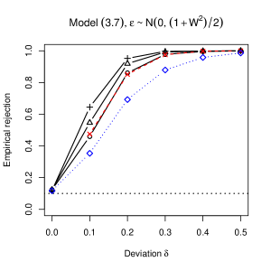
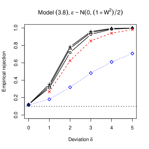
Figure 2: Power curves for models (3.7) and (3.8), $n=100$.

where $\widetilde{\sigma}^{2}=\frac{2\tau^{2}\left(1-\tau\right)^{2}}{n(n-1)}\sum_{j\neq i}h^{-q}\tilde{K}^{2}\left(\dfrac{W_{i}-W_{j}}{h},\,\dfrac{X_{i}-X_{j}}{h}\right)$, and $\tilde{K}$ is a triangle kernel applied to the norm of its argument. We apply the wild bootstrap procedure to compute the critical values of all tests. Figure 2 reports power curves of the different tests as a function of $\delta$ based on $2500$ replications. For the linear Model (3.7), all tests perform almost similarly. Our test is a bit more powerful, especially for a larger bandwidth, which was expected given our theoretical analysis. For the nonlinear Model (3.8), the power advantage of our test is more pronounced. Its power can be as large as twice the power of the test by He and Zhu (2003).

3.2 Empirical Illustration

We studied some parametric quantile models for children birthweight using data analyzed by Abrevaya (2001) and Koenker and Hallock (2001), who gave a detailed data description. We focused on median regression and the 10th percentile quantile regression. Models are estimated and tested on a subsample of 1168 smoking college graduate mothers. We first analyzed the simple model considered by He and Zhu (2003), which is linear in weight gain during pregnancy (WTGAIN), average number of cigarettes per day (CIGAR), and age (AGE). When implementing our test, we chose age as the $W$ variable, and we standardize all explanatory variables. Other details are identical to what was done in simulations. For both quantiles, HZ test does not reject this specification. Our test does not reject the linear median regression at 10% level, but detects misspecification for the lower decile regression when $c=2$.

Since the more detailed analysis of Abrevaya (2001) and Koenker and Hallock (2001) suggests that birthweight is quadratic in age, we then considered this variation. None of the tests detects a misspecified model. Finally, we considered a more complete model similar to Abrevaya (2001), where we added the explanatory binary variables BOY (1 if child is male), BLACK (1 if mother is black), MARRIED (1 if married), and NOVISIT (1 if no prenatal visit during the pregnancy). HZ test does not reject the model at either quantiles. Our test however indicates a misspecified median regression model at 10% level, while it does not reject the model for the lower decile. Our limited empirical exercice suggests that our new test, beside existing procedures such as the test by He and Zhu (2003), is a valuable addition to the practitioner toolbox.

4 Proofs

We first recall some definitions. For the definition of a VC-class, we refer to Section 2.6.2 of van der Vaart and Wellner (1996). Next, let $\mathcal{G}$ be a class of real-valued functions on a set $\mathcal{S}$. We call $\mathcal{G}$ an Euclidean(c,d) family of functions, or simply Euclidean, for the envelope $G$ if there exists positive constants $c$ and $d$ with the following properties: if $0<\epsilon\leq 1$ and $\lambda$ is a measure for which $\int G^{2}d\lambda<\infty$, then there are functions $g_{1},\dots,g_{j}$ in $\mathcal{G}$ such that (i) $j\leq c\epsilon^{-d}$; and (ii) for each $g$ in $\mathcal{G}$ there is an $g_{i}$ with $\int|g-g_{i}|^{2}d\lambda\leq\epsilon^{2}\int G^{2}d\lambda$. The constants $c$ and $d$ must not depend on $\lambda$. See e.g. Nolan and Pollard (1987) or Sherman (1994). Recall that if $\mathcal{F}$ is a VC-class of functions then the class $\{\mathbb{I}\{f\geq 0\}:f\in\mathcal{F}\}$ is Euclidean for the envelope $F\equiv 1$, see van der Vaart and Wellner (1996) Lemma 2.6.18(iii) and Theorem 2.6.7 or Pakes and Pollard (1989). Bellow, we shall use this property with the VC-classes of functions of $\{\varepsilon+g(Z,\beta_{0})-g(Z,\beta):\beta\in B\}$ and $\{\varepsilon+g(Z,\beta_{0})+r_{n}\delta(Z)-g(Z,\beta):\beta\in B\}$.

In the following, $F_{\varepsilon}\left(\cdot\mid x\right)$ is the conditional distribution function of $\varepsilon$ given $Z=z;$ that means $F_{\varepsilon}\left(0\mid\cdot\right)\equiv\tau$. Below $C$, $C_{1}$, $C_{2}$,… denote constants, not necessarily the same as before and possibly changing from line to line.

4.1 Proof of Theorem 2.2

Proof. First, we prove that if $\mathcal{H}_{0}$ holds

$$n\sqrt{h}\left\{W_{n}(\widehat{\beta})-W_{n}(\beta_{0})\right\}=o_{\mathbb{P}}\left(1\right).$$ (4.1)

Let us introduce some simplifying notation:

$$G_{i}\left(\beta,\beta_{0}\right)=g(Z_{i};\beta)-g(Z_{i};\beta_{0}),\,\,\,\psi_{ij}=\psi(X_{i}-X_{j}),\,\,\,K_{h,ij}=K_{h}\left(W_{i}-W_{j}\right).$$ (4.2)

Under $\mathcal{H}_{0}$

$$W_{n}(\beta) = \frac{h^{-1}}{n(n-1)}\sum\limits_{j\neq i}\left[\mathbb{I}\{Y_{i}\leq g(Z_{i};\beta)\}-\tau\right]\left[\mathbb{I}\{Y_{j}\leq g(Z_{j};\beta)\}-\tau\right]K_{h,ij}\psi_{ij}$$

$$= \frac{h^{-1}}{n(n-1)}\sum\limits_{j\neq i}\left[\mathbb{I}\{\varepsilon_{i}\leq G_{i}(\beta,\beta_{0})\}-F_{\varepsilon}\left(0\mid Z_{i}\right)\right]$$

$$\qquad\qquad\qquad\qquad\qquad\times\left[\mathbb{I}\{\varepsilon_{j}\leq G_{j}(\beta,\beta_{0})\}-F_{\varepsilon}\left(0\mid Z_{j}\right)\right]K_{h,ij}\psi_{ij}.$$

By a Taylor expansion, decompose

$$F_{\varepsilon}\left(0\mid Z_{i}\right)=F_{\varepsilon}\left(G_{i}(\beta,\beta_{0})\mid Z_{i}\right)-f_{\varepsilon}\left(0\mid Z_{i}\right)\dot{g}^{\prime}(Z_{i};\beta_{0})\left(\beta-\beta_{0}\right)+O_{\mathbb{P}}\left(\left\|\beta-\beta_{0}\right\|^{2}\right).$$

We can write $W_{n}(\beta)-W_{n}(\beta_{0})=\{W_{1n}^{0}(\beta)-W_{1n}^{0}(\beta_{0})\}+2W_{2n}^{0}(\beta)+W_{3n}^{0}(\beta)+R_{n}^{0}$ where

$$W_{1n}^{0}(\beta)=\frac{h^{-1}}{n(n-1)}\!\sum\limits_{j\neq i}\left[\mathbb{I}\{\varepsilon_{i}\leq G_{i}(\beta,\beta_{0})\}-F_{\varepsilon}\left(G_{i}(\beta,\beta_{0})\mid Z_{i}\right)\right]\\ \times\left[\mathbb{I}\{\varepsilon_{j}\leq G_{j}(\beta,\beta_{0})\}-F_{\varepsilon}\left(G_{j}(\beta,\beta_{0})\mid Z_{j}\right)\right]K_{h,ij}\psi_{ij}$$

$W_{2n}^{0}(\beta)=\left(\beta-\beta_{0}\right)^{\prime}\widetilde{W}_{2n}^{0}(\beta)$ with

$$\widetilde{W}_{2n}^{0}(\beta) = \frac{h^{-1}}{n(n-1)}\sum\limits_{j\neq i}\left[\mathbb{I}\{\varepsilon_{i}\leq G_{i}(\beta,\beta_{0})\}-F_{\varepsilon}\left(G_{i}(\beta,\beta_{0})\mid Z_{i}\right)\right]$$

$$\qquad\qquad\qquad\qquad\times f_{\varepsilon}\left(0\mid Z_{j}\right)\dot{g}(Z_{j};\beta_{0})K_{h,ij}\psi_{ij},$$

$W_{3n}^{0}(\beta)=\left(\beta-\beta_{0}\right)^{\prime}\widetilde{W}_{3n}^{0}\left(\beta-\beta_{0}\right)$ with

$$\widetilde{W}_{3n}^{0}=\frac{h^{-1}}{n(n-1)}\sum\limits_{j\neq i}f_{\varepsilon}\left(0\mid Z_{i}\right)\dot{g}(Z_{i};\beta_{0})\dot{g}^{\prime}(Z_{j};\beta_{0})f_{\varepsilon}\left(0\mid Z_{j}\right)K_{h,ij}\psi_{ij}=O_{\mathbb{P}}(1).\$$

The rate of $\widetilde{W}_{3n}^{0}$ follows simply by computing its mean and variance. By Assumption 2.1(c) and Assumption 2.2(c) it is easy to check that $\left|R_{n}^{0}\right|\leq\left\|\beta-\beta_{0}\right\|^{2}O_{\mathbb{P}}\left(1\right).$ For deriving the order of $\widetilde{W}_{2n}^{0},$ apply Hoeffding decomposition and write $h\widetilde{W}_{2n}^{0}(\beta)=V_{n}^{2}(\beta)+V_{n}^{1}(\beta)$ with $V_{n}^{1}$, $V_{n}^{2}$ degenerate $U-$processes or order 1 and 2, respectively. In view of Assumptions 2.2(d) and 2.3(a), apply Corollary 4 of Sherman (1994) and deduce that $V_{n}^{2}(\beta)=O_{\mathbb{P}}\left(n^{-1}\right)$ uniformly in $\beta$ (and $h$). Next, if $\dot{g}^{\left(l\right)}$ denotes the $l$th component of the vector of first-order derivatives $\dot{g},$ $1\leq l\leq p,$ and

$$\pi^{\left(l\right)}\left(Z_{i}\right)=\mathbb{E}\left[f_{\varepsilon}\left(0\mid Z_{j}\right)\dot{g}^{\left(l\right)}(Z_{j};\beta_{0})h^{-3/4}K_{h,ij}\psi_{ij}\mid Z_{i}\right]$$

we can rewrite the $l$th component of the vector $V_{n}^{1}(\beta)$ as

$$\frac{h^{3/4}}{n}\sum\limits_{i=1}^{n}\left[\mathbb{I}\{\varepsilon_{i}\leq G_{i}(\beta,\beta_{0})\}-F_{\varepsilon}\left(G_{i}(\beta,\beta_{0})\mid Z_{i}\right)\right]\pi^{\left(l\right)}\left(Z_{i}\right).$$

By Hölder inequality, Assumption 2.1(c), Assumption 2.2(c) and a change of variables,

$$\left|\pi^{\left(l\right)}\left(X_{i}\right)\right| \leq \mathbb{E}\left[f_{\varepsilon}\left(0\mid Z_{j}\right)\left|\dot{g}^{\left(l\right)}(Z_{j};\beta_{0})\right|h^{-3/4}K_{h,ij}\left|\psi_{ij}\right|\mid Z_{i}\right]$$

$$\leq C_{1}\mathbb{E}^{1/4}\left[A^{4}(Z_{j})\right]\mathbb{E}^{3/4}\left[h^{-1}K_{h,ij}^{4/3}\mid Z_{i}\right]$$

$$\leq C_{2},$$

for any $1\leq l\leq p.$ Now, by Corollary 4 of Sherman (1994), $h^{-3/4}V_{n}^{1}(\beta)=O_{\mathbb{P}}\left(n^{-1/2}\right)$ uniformly in $\beta.$ Deduce that

$$\sup_{\beta}|W_{2n}^{0}(\beta)|\leq\left\|\beta-\beta_{0}\right\|O_{\mathbb{P}}\left(h^{-1}n^{-1}+h^{-1/4}n^{-1/2}\right).$$

Finally, by Lemma 1 of Zheng (1998), for any $\alpha\in(0,1)$

$$\sup_{\beta}|W_{1n}^{0}(\beta)-W_{1n}^{0}(\beta_{0})|=O_{\mathbb{P}}\left(h^{-1}n^{-1-\alpha/4}\right)$$

uniformly over $O_{\mathbb{P}}\left(n^{-1/2}\right)$ neighborhoods of $\beta_{0}.$ Gathering the results and using Lemma 4.1 with $\delta(\cdot)\equiv 0$ we obtain (4.1). Now, it remains to check that $nh^{1/2}W_{n}(\beta_{0})/v_{n}$ converges in law to a standard normal distribution. This result easily follows as a particular case of Lemma 4.1 below.   

4.2 Proof of Theorem 2.3

First, we derive the behavior of $\widehat{\beta},$ the estimator of $\beta_{0}$ under the sequence of local alternatives $H_{\!1n}.$

Lemma 4.1

Suppose that Assumptions 2.1, 2.2 hold, let $\delta(\cdot)$ be a function such that Condition (2.6) holds, and let $r_{n}$, $n\geq 1$ be a sequence of real numbers such that $r_{n}\rightarrow 0$. If $\widehat{\beta}=\arg\min_{\beta\in B}\!\Gamma_{n}\left(\beta\right)$ with $\Gamma_{n}\left(\beta\right)=\!\!\sum_{i=1}^{n}\rho_{\tau}(Y_{i}-\!g(Z_{i};\beta))$, then under $\mathcal{H}_{0},$ $\widehat{\beta}-\!\beta_{0}\!=\!O_{\mathbb{P}}(n^{-1/2})$ and under $H_{\!1n}$ defined in (2.5), $\widehat{\beta}-\beta_{n}=O_{\mathbb{P}}(n^{-1/2})$ where

$$\beta_{n}=\beta_{0}-r_{n}^{2}\left[\mathbb{E}\left[f_{\varepsilon}(0\mid Z\,)\dot{g}(Z;\beta_{0})\dot{g}^{\prime}(Z;\beta_{0})\right]\right]^{-1}\mathbb{E}\left[f_{\varepsilon}^{\,\prime}(0\mid Z)\delta^{2}(Z)\dot{g}(Z;\beta_{0})\right].$$

Proof. It is easy to check that

$$\left|\rho_{\tau}\left(a-b\right)-\rho_{\tau}\left(a\right)\right|\leq\left|b\right|\max\left(\tau,1-\tau\right)\leq\left|b\right|.$$ (4.3)

Combine this with the Mean Value Theorem and Assumption 2.2(c) to check the conditions of Lemma 2.13 of Pakes and Pollard (1989) and to derive the Euclidean property for an integrable envelope for the family of functions $\left\{\left(y,z\right)\!\mapsto\!\rho_{\tau}(y-\!g(z;\beta))\!:\beta\in B\right\}.$

Next, we study the consistency of $\widehat{\beta}$ under $H_{0}$. By the uniform law of large numbers, $\sup_{\beta}\left|n^{-1}\Gamma_{n}\left(\beta\right)-\mathbb{E}\left[\rho_{\tau}(Y-g(Z;\beta))\right]\right|\rightarrow 0,$ in probability (use for instance Lemma 2.8 of Pakes and Pollard 1989). This uniform convergence, the identification condition in Assumption 2.2(a), the continuity of $g\left(z;\cdot\right)$ for any $z,$ and usual arguments used for proving consistency of argmax estimators, allow to deduce $\widehat{\beta}-\beta_{0}=o_{\mathbb{P}}(1).$ To obtain the consistency under the local alternatives approaching $H_{0}$, it suffices to prove $\sup_{\beta\in B}\left|\Delta_{n}\left(\beta\right)\right|\rightarrow 0$ in probability, where

$$\Delta_{n}\left(\beta\right)=\frac{1}{n}\sum_{i=1}^{n}\left\{\rho_{\tau}\left(l(\varepsilon_{i},Z_{i};\beta)+r_{n}\delta(Z_{i})\right)-\rho_{\tau}\left(l(\varepsilon_{i},Z_{i};\beta)\right)\right\}$$

and $l(u,z;\beta)=u+g(z;\beta_{0})-g(z;\beta).$ By inequality (4.3),

$$\left|\Delta_{n}\left(\beta\right)\right|\leq\frac{\left|r_{n}\right|}{n}\sum_{i=1}^{n}\left|\delta(Z_{i})\right|.$$

Consequently, $\Delta_{n}\left(\beta\right)=o_{\mathbb{P}}(1)$ uniformly over $\beta\in B$, and thus the consistency follows.

Define $\psi_{\tau}(e)=\tau-\mathbb{I}(e<0)$ as the derivative of $\rho_{\tau}.$ To obtain the rate of convergence of $\widehat{\beta}$ under $\mathcal{H}_{1n}$ (in particular under $H_{0}$ by taking $r_{n}\equiv 0$) consider the empirical process

$$\nu_{n}\left(\beta\right)=\frac{1}{\sqrt{n}}\sum_{i=1}^{n}\left\{\psi_{\tau}\left(Y_{i}-g(Z_{i};\beta)\right)-\mathbb{E}[\psi_{\tau}\left(Y_{i}-g(Z_{i};\beta)\right)\mid Z_{i}]\right\}\dot{g}(Z_{i};\beta)\\ =\frac{1}{\sqrt{n}}\sum_{i=1}^{n}\left\{\psi_{\tau}\left(l(\varepsilon_{i},Z_{i};\beta)+r_{n}\delta(Z_{i})\right)-\mathbb{E}\left[\psi_{\tau}\left(l(\varepsilon_{i},Z_{i};\beta)+r_{n}\delta(Z_{i})\right)\mid Z_{i}\right]\right\}\dot{g}(Z_{i};\beta)$$

indexed by $\beta.$ First, let us notice that

$$\nu_{n}\left(\beta\right)-\nu_{n}\left(\beta_{0}\right)=o_{\mathbb{P}}\left(1\right)$$ (4.4)

uniformly over $o_{\mathbb{P}}\left(1\right)$ neighborhoods of $\beta_{0},$ as a consequence of Corollary 8 of Sherman (1994). Indeed, by Lemma 2.13 of Pakes and Pollard (1989), the class of functions $\{\dot{g}(\cdot;\beta):\beta\in B\}$ is Euclidean for a squared integrable envelope. Next, by the VC-class property of the regression functions $\{g(\cdot;\beta)$, $\beta\in B\}$, the class of functions $\{(u,z)\mapsto\psi_{\tau}\left(l(u,z;\beta)+r_{n}\delta(z)\right):\beta\in B\}$ is Euclidean(c,d) for a constant envelope. See Lemma 2.12 of Pakes and Pollard (1989). Moreover, the constants $c$ and $d$ can be taken independent of $n$, see, for instance, the proof of Lemma 2.6.18(v) of van der Vaart and Wellner (1996). Finally, by repeated applications of the Mean Value Theorem and Assumptions 2.1(c) and 2.2(c), for any $z,\beta_{1},\beta_{2}$ we have

$$\hskip-28.45274pt\left|\,\mathbb{E}\left[\psi_{\tau}\left(l(\varepsilon,z;\beta_{1})+r_{n}\delta(z)\right)\right]-\mathbb{E}\left[\psi_{\tau}\left(l(\varepsilon,z;\beta_{2})+r_{n}\delta(z)\right)\right]\,\right|$$

$$\leq \left|F_{\varepsilon}\left(g(z;\beta_{1})-g(z;\beta_{0})-r_{n}\delta(z)\mid z\right)-F_{\varepsilon}\left(g(z;\beta_{2})-g(z;\beta_{0})-r_{n}\delta(z)\mid z\right)\right|$$

$$\leq f_{\varepsilon}(v_{n}\mid z)\left|g(z;\beta_{1})-g(z;\beta_{2})\right|$$

$$\leq CA\left(z\right)\left\|\beta_{1}-\beta_{2}\right\|$$

for some $v_{n}$ between $g(z;\beta_{1})-g(z;\beta_{0})-r_{n}\delta(z)$ and $g(z;\beta_{2})-g(z;\beta_{0})-r_{n}\delta(z).$ By Pakes and Pollard (1989, Lemma 2.13), the class of functions $\{z\mapsto\mathbb{E}\left[\psi_{\tau}\left(l(\varepsilon,z;\beta)+r_{n}\delta(z)\right)\right]:\beta\in B\}$ is Euclidean(c,d) for an envelope with a finite fourth moment, with $c$ and $d$ independent of $n$. Deduce that the empirical process $\nu_{n}\left(\beta\right)$, $\beta\in B$, is indexed by a class of functions that is Euclidean for a squared integrable envelope. Finally, condition (ii) of Corollary 8 of Sherman (1994), can be checked from inequalities like in (4.2) and conditions on $\left|\dot{g}(z;\beta)-\dot{g}(z;\beta_{0})\right|$.

On the other hand, because $\widehat{\beta}$ minimizes $\Gamma_{n}\left(\beta\right)$ defined in (2.3) over $\beta$, the directional derivative of $\Gamma_{n}\left(\beta\right)$ at $\widehat{\beta}$ along any direction $\gamma$ (with $\left\|\gamma\right\|=1$) is nonnegative. That is

$$0 \leq \lim_{t\rightarrow 0}t^{-1}\left[\Gamma_{n}(\widehat{\beta}+t\gamma)-\Gamma_{n}(\widehat{\beta})\right]$$

$$= -\sum_{\left\{Y_{i}\neq g(Z_{i};\widehat{\beta})\right\}}\psi_{\tau}\left(Y_{i}-g(Z_{i};\widehat{\beta})\right)\gamma\,^{\prime}\dot{g}(Z_{i};\widehat{\beta})$$

$$+\lim_{t\rightarrow 0}\sum_{\left\{Y_{i}=g(Z_{i};\widehat{\beta})\right\}}t^{-1}\rho_{\tau}\left(g(Z_{i};\widehat{\beta})-g(Z_{i};\widehat{\beta}+t\gamma)\right)$$

$$= -\sum_{\left\{Y_{i}\neq g(Z_{i};\widehat{\beta})\right\}}\psi_{\tau}\left(Y_{i}-g(Z_{i};\widehat{\beta})\right)\gamma\,^{\prime}\dot{g}(Z_{i};\widehat{\beta})$$

$$-\sum_{\left\{Y_{i}=g(Z_{i};\widehat{\beta})\right\}}\psi_{\tau}\left(-\gamma\,^{\prime}\dot{g}(Z_{i};\widehat{\beta})\right)\gamma\,^{\prime}\dot{g}(Z_{i};\widehat{\beta})$$

$$= -D_{1n}(\widehat{\beta})-D_{2n}(\widehat{\beta}).$$

By Assumption 2.2, $|D_{2n}(\widehat{\beta})|$ is bounded by $\sum_{\left\{Y_{i}=g(Z_{i};\widehat{\beta})\right\}}A(Z_{i}).$ As, for any $x$, the error term $u$ has a continuous law given $Z=z$, the number of observations with $Y_{i}=g(Z_{i};\widehat{\beta})$ is bounded in probability as the sample size tends to infinity. On the other hand, the moment condition on $A\left(\cdot\right)$ implies that $\max_{1\leq i\leq n}A(Z_{i})=o_{\mathbb{P}}\left(n^{1/2}\right).$ As $\gamma$ is an arbitrary direction, it follows that

$$\frac{1}{\sqrt{n}}\sum_{i=1}^{n}\psi_{\tau}\left(Y_{i}-g(Z_{i};\widehat{\beta})\right)\dot{g}(Z_{i};\widehat{\beta})=o_{\mathbb{P}}\left(1\right).$$ (4.7)

Finally, since $\widehat{\beta}-\beta_{0}=o_{\mathbb{P}}\left(1\right)$ and $\tau=F_{\varepsilon}(0\mid Z_{i})$, deduce that

$$\nu_{n}\left(\beta_{0}\right) = \nu_{n}(\widehat{\beta})+o_{\mathbb{P}}\left(1\right)\hskip 256.0748pt\text{[by (\ref{negli1})]}$$

$$= -\frac{1}{\sqrt{n}}\sum_{i=1}^{n}\mathbb{E}\left[\psi_{\tau}\left(Y_{i}-g(Z_{i};\widehat{\beta})\right)\mid Z_{i}\right]\dot{g}(Z_{i};\widehat{\beta})+o_{\mathbb{P}}\left(1\right)\hskip 51.21504pt\text{[by (\ref{negli2})]}$$

$$= \frac{1}{\sqrt{n}}\sum_{i=1}^{n}\left[F_{\varepsilon}\left(g(\,Z_{i};\widehat{\beta}\,)-g(Z_{i};\beta_{0})-r_{n}\delta(\,Z_{i}\,)\mid Z_{i}\right)-\tau\right]\dot{g}(Z_{i};\widehat{\beta})+o_{\mathbb{P}}\left(1\right)$$

$$= \left\{\frac{1}{n}\sum_{i=1}^{n}f_{\varepsilon}(0\mid Z_{i})\dot{g}(Z_{i};\beta_{0})\dot{g}^{\prime}(Z_{i};\beta_{0})\right\}\sqrt{n}\left(\widehat{\beta}-\beta_{0}\right)$$

$$-r_{n}\left\{\frac{1}{\sqrt{n}}\sum_{i=1}^{n}f_{\varepsilon}(0\mid Z_{i})\delta(\,Z_{i}\,)\dot{g}(Z_{i};\beta_{0})\right\}$$

$$+r_{n}^{2}\sqrt{n}\left\{\frac{1}{n}\sum_{i=1}^{n}f_{\varepsilon}^{\,\prime}(0\mid Z_{i})\delta^{2}(\,Z_{i}\,)\dot{g}(Z_{i};\beta_{0})\right\}$$

$$+o_{\mathbb{P}}\left(\sqrt{n}\|\widehat{\beta}-\beta_{0}\|\right)+o_{\mathbb{P}}\left(r_{n}^{2}\sqrt{n}\right),$$

where the last equality is based on a local expansions of $F_{\varepsilon}\left(\cdot\mid z\right)$ and $g(z;\cdot).$ By the law of large numbers, the central limit theorem and the fact that $\nu_{n}\left(\beta_{0}\right)=O_{\mathbb{P}}\left(1\right)$ and the random vector $f_{u}(0\mid Z)\delta(\,Z\,)\dot{g}(Z;\beta_{0})$ has zero mean, we obtain

$$\mathbb{E}[f_{\varepsilon}(0\mid Z)\dot{g}(Z;\beta_{0})\dot{g}^{\prime}(Z;\beta_{0})]\sqrt{n}\left(\widehat{\beta}-\beta_{0}\right)+r_{n}^{2}\sqrt{n}\mathbb{E}[f_{\varepsilon}^{\,\prime}(0\mid Z)\delta^{2}(Z)\dot{g}(Z;\beta_{0})]=O_{\mathbb{P}}(1)$$

from which the result follows.   

Lemma 4.1 shows in particular that under $\mathcal{H}_{1n},$ $\widehat{\beta}-\beta_{0}=O_{\mathbb{P}}(n^{-1/2}+r_{n}^{2}).$ To our best knowledge, this result on the behavior of $\widehat{\beta}$ under the local alternatives is new. He and Zhu (2003) only considered the case $r_{n}=n^{-1/2}$ while Zheng (1998) assumed $\widehat{\beta}-\beta^{\ast}=O_{\mathbb{P}}(n^{-1/2})$ under $\mathcal{H}_{1n}$, for some fixed $\beta^{\ast}$. Our Lemma 4.1 indicates that such $\sqrt{n}-$convergence assumptions on the local alternatives may be too restrictive. Below, we improve the point (C) in the Theorem of Zheng (1998) also because we can take into account the rates of convergence of $\widehat{\beta}$ under the alternatives slower than $O_{\mathbb{P}}(n^{-1/2})$.

In the case of a fixed deviation from the null hypothesis, that is $r_{n}\equiv 1,$ the tools used for proving Theorem 2.3 could be easily adapted to show the $\sqrt{n}-$convergence of $\widehat{\beta}$ to $\beta^{*}$ that minimizes the map $\beta\mapsto\mathbb{E}[\rho_{\tau}(Y-g(Z,\beta))]=\mathbb{E}[\rho_{\tau}(g(Z,\beta_{0})+\delta(Z)+\varepsilon-g(Z,\beta))].$ The consistency of the test is then a consequence of the fact that $nh^{1/2}I_{n}(\beta^{*})$ tends to infinity.

Let $\delta_{i}=\delta(Z_{i})$ and let $G_{i}\left(\beta,\beta_{0}\right)$ and $K_{h,ij}$ be defined as in equation (4.2). Under $\mathcal{H}_{1n}$

$$W_{n}(\beta) = \frac{h^{-1}}{n(n-1)}\sum\limits_{j\neq i}\left[\mathbb{I}\{Y_{i}\leq g(Z_{i};\beta)\}-\tau\right]\left[\mathbb{I}\{Y_{j}\leq g(Z_{j};\beta)\}-\tau\right]K_{h,ij}\psi_{ij}$$

$$= \frac{h^{-1}}{n(n-1)}\sum\limits_{j\neq i}\left[\mathbb{I}\{\varepsilon_{i}\leq G_{i}(\beta,\beta_{0})-r_{n}\delta_{i}\}-F_{\varepsilon}\left(0\mid Z_{i}\right)\right]$$

$$\qquad\qquad\qquad\times\left[\mathbb{I}\{\varepsilon_{j}\leq G_{j}(\beta,\beta_{0})-r_{n}\delta_{j}\}-F_{\varepsilon}\left(0\mid Z_{j}\right)\right]K_{h,ij}\psi_{ij}.$$

Let us decompose

$$F_{\varepsilon}\left(0\mid Z_{i}\right) = F_{\varepsilon}\left(G_{i}(\beta,\beta_{0})-r_{n}\delta_{i}\mid Z_{i}\right)-f_{\varepsilon}\left(0\mid Z_{i}\right)\left\{\dot{g}^{\prime}(Z_{i};\beta_{0})\left(\beta-\beta_{0}\right)-r_{n}\delta_{i}\right\}$$

$$\qquad-2^{-1}r_{n}^{2}f_{\varepsilon}^{\,\prime}\left(0\mid Z_{i}\right)\delta_{i}^{2}+O_{\mathbb{P}}\left(\left\|\beta-\beta_{0}\right\|^{2}+r_{n}\left\|\beta-\beta_{0}\right\|\right)+o_{\mathbb{P}}\left(r_{n}^{2}\right).$$

We can write

$$W_{n}(\beta)=W_{1n}(\beta)+2[W_{2n}(\beta)+W_{3n}(\beta)+W_{4n}(\beta)]+W_{5n}(\beta)+2W_{6n}(\beta)+W_{7n}+R_{n}$$

where

$$W_{1n}(\beta)=\frac{h^{-1}}{n(n-1)}\!\sum\limits_{j\neq i}\left[\mathbb{I}\{\varepsilon_{i}\leq G_{i}(\beta,\beta_{0})-r_{n}\delta_{i}\}-F_{\varepsilon}\left(G_{i}(\beta,\beta_{0})-r_{n}\delta_{i}\mid Z_{i}\right)\right]\\ \times\left[\mathbb{I}\{\varepsilon_{j}\leq G_{j}(\beta,\beta_{0})-r_{n}\delta_{j}\}-F_{\varepsilon}\left(G_{j}(\beta,\beta_{0})-r_{n}\delta_{j}\mid Z_{j}\right)\right]K_{h,ij}\psi_{ij}$$

$W_{2n}(\beta)=\left(\beta-\beta_{0}\right)^{\prime}\widetilde{W}_{2n}(\beta)$ with

$$\widetilde{W}_{2n}(\beta) = \frac{h^{-1}}{n(n-1)}\sum\limits_{j\neq i}\left[\mathbb{I}\{\varepsilon_{i}\leq G_{i}(\beta,\beta_{0})-r_{n}\delta_{i}\}-F_{\varepsilon}\left(G_{i}(\beta,\beta_{0})-r_{n}\delta_{i}\mid Z_{i}\right)\right]$$

$$\qquad\qquad\qquad\times f_{\varepsilon}\left(0\mid Z_{j}\right)\dot{g}(Z_{j};\beta_{0})K_{h,ij}\psi_{ij},$$

$$W_{3n}(\beta) = \frac{r_{n}h^{-1}}{n(n-1)}\sum\limits_{j\neq i}\left[\mathbb{I}\{\varepsilon_{i}\leq G_{i}(\beta,\beta_{0})-r_{n}\delta_{i}\}-F_{\varepsilon}\left(G_{i}(\beta,\beta_{0})-r_{n}\delta_{i}\mid Z_{i}\right)\right]$$

$$\qquad\qquad\qquad\times f_{\varepsilon}\left(0\mid Z_{j}\right)\delta_{j}K_{h,ij}\psi_{ij},$$

$$W_{4n}(\beta) = \frac{r_{n}^{2}h^{-1}}{2n(n-1)}\sum\limits_{j\neq i}\left[\mathbb{I}\{\varepsilon_{i}\leq G_{i}(\beta,\beta_{0})-r_{n}\delta_{i}\}-F_{\varepsilon}\left(G_{i}(\beta,\beta_{0})-r_{n}\delta_{i}\mid Z_{i}\right)\right]$$

$$\qquad\qquad\qquad\times f_{\varepsilon}^{\,\prime}\left(0\mid Z_{j}\right)\delta_{j}^{2}K_{h,ij}\psi_{ij},$$

$W_{5n}(\beta)=\left(\beta-\beta_{0}\right)^{\prime}\widetilde{W}_{5n}\left(\beta-\beta_{0}\right)$ with

$$\widetilde{W}_{5n}=\frac{h^{-1}}{n(n-1)}\sum\limits_{j\neq i}f_{\varepsilon}\left(0\mid Z_{i}\right)\dot{g}(Z_{i};\beta_{0})\dot{g}^{\prime}(Z_{j};\beta_{0})f_{\varepsilon}\left(0\mid Z_{j}\right)K_{h,ij}\psi_{ij}=O_{\mathbb{P}}(1),$$

$W_{6n}(\beta)=\left(\beta-\beta_{0}\right)^{\prime}\widetilde{W}_{6n}$ with

$$\widetilde{W}_{6n}=\frac{r_{n}h^{-1}}{n(n-1)}\sum\limits_{j\neq i}f_{\varepsilon}\left(0\mid Z_{i}\right)\delta_{i}f_{\varepsilon}\left(0\mid Z_{j}\right)\dot{g}(X_{j};\beta_{0})K_{h,ij}\psi_{ij}=O_{\mathbb{P}}(r_{n}),$$

$$W_{7n}=\frac{r_{n}^{2}h^{-1}}{n(n-1)}\sum\limits_{j\neq i}f_{\varepsilon}\left(0\mid Z_{i}\right)\delta(X_{i})f_{\varepsilon}\left(0\mid Z_{j}\right)\delta(Z_{j})K_{h,ij}\psi_{ij}=C_{1}r_{n}^{2}+o_{\mathbb{P}}(r_{n}^{2})$$

with $C_{1}>0$ and $R_{n}$ a reminder term that is negligible because of the properties of $f_{\varepsilon}^{\,\prime}$ and $\dot{g}$. Note that the $U-$statistics $\widetilde{W}_{5n}$, $\widetilde{W}_{6n}$ and $W_{7n}$ depend only on the $X_{i}.$ Their orders are obtained from elementary calculations of mean and variance.

Next, we can write $W_{1n}(\beta)=\left\{W_{1n}(\beta)-W_{1n}(\beta_{0})\right\}+W_{1n}(\beta_{0}).$ As $W_{1n}(\beta_{0})$ is centered, its order in probability is given by the variance. We have

$$\mbox{\rm Var}(W_{1n}(\beta_{0})\mid Z_{1},...,Z_{n}) = \frac{1}{n^{2}(n-1)^{2}}\sum_{i\neq j}F_{\varepsilon}\left(-r_{n}\delta_{i}\mid Z_{i}\right)[1-F_{\varepsilon}\left(-r_{n}\delta_{i}\mid Z_{i}\right)]$$

$$\,\,\,\,\,\times F_{\varepsilon}\left(-r_{n}\delta_{j}\mid Z_{j}\right)[1-F_{\varepsilon}\left(-r_{n}\delta_{j}\mid Z_{j}\right)]h^{-2}K_{h,ij}^{2}\psi_{ij}\left(\mu\right)$$

$$\leq \frac{h^{-1}}{16n(n-1)}\left[\frac{1}{n(n-1)}\sum_{i\neq j}h^{-1}K_{h,ij}^{2}\psi_{ij}\right]$$

The expectation of the last $U-$statistic in the display converges to a constant while the variance tends to zero. As $W_{1n}(\beta_{0})$ is of zero conditional mean given the $Z_{i}$, deduce that the variance of $W_{1n}(\beta_{0})$ is bounded by $Cn^{-2}h^{-1}$. By Chebyshev’s inequality, $W_{1n}(\beta_{0})=o_{\mathbb{P}}\left(r_{n}^{2}\right)$, provided that $r_{n}^{2}nh^{1/2}\rightarrow\infty.$ Next, let

$$H_{1n}(Z_{i},Z_{j},\beta)=\left[\mathbb{I}\{\varepsilon_{i}\leq G_{i}(\beta,\beta_{0})-r_{n}\delta_{i}\}-F_{\varepsilon}\left(G_{i}(\beta,\beta_{0})-r_{n}\delta_{i}\mid Z_{i}\right)\right]\\ \times\left[\mathbb{I}\{\varepsilon_{j}\leq G_{j}(\beta,\beta_{0})-r_{n}\delta_{j}\}-F_{\varepsilon}\left(G_{j}(\beta,\beta_{0})-r_{n}\delta_{j}\mid Z_{j}\right)\right]K_{h,ij}\psi_{ij},\qquad\beta\in B.$$

By the arguments used for Lemma 4.1 above, the class of functions $\{H_{1n}(\cdot,\cdot,\beta):\beta\in B\}$ is Euclidean(c,d) for an envelope with a finite fourth moment, with $c$ and $d$ independent of $n$. Now, we can use equation (A.11) of Zheng (1998) and his Lemma 1 with the condition (ii) replaced by $\mathbb{E}[H_{1n}(\cdot,\beta)-H_{1n}(\cdot,\beta_{0})]^{2}\leq\Lambda\left\|\beta-\beta_{0}\right\|$. By a close inspection of the proof of Zheng’s Lemma 1, see his equations (A.2) to (A.5), it is obvious to adapt his conclusion and to deduce that in our setup for any $0<\alpha<1$

$$W_{1n}(\beta)-W_{1n}(\beta_{0})=O_{\mathbb{P}}\left(n^{-1}h^{-1}\left\|\beta-\beta_{0}\right\|^{\alpha/2}\right)=O_{\mathbb{P}}\left(n^{-1}h^{-1}\left\{r_{n}+n^{-1/4}\right\}^{\alpha}\right)$$

uniformly over $O_{\mathbb{P}}(r_{n}^{2}+n^{-1/2})$ neighborhoods of $\beta_{0}.$ Thus, when $n^{1/2}r_{n}^{2}\rightarrow\infty,$ we have

$$W_{1n}(\widehat{\beta})-W_{1n}(\beta_{0})=O_{\mathbb{P}}\left(n^{-1}h^{-1}r_{n}^{\alpha}\right)=O_{\mathbb{P}}\left(n^{-1/2}\right)=o_{\mathbb{P}}\left(r_{n}^{2}\right),$$

whereas in the case where $n^{1/2}r_{n}^{2}$ is bounded, use $nh^{1/2}r_{n}^{2}\rightarrow\infty$ and take $\alpha$ sufficiently close to one to obtain

$$W_{1n}(\widehat{\beta})-W_{1n}(\beta_{0})=O_{\mathbb{P}}\left(n^{-1-\alpha/4}h^{-1}\right)=o_{\mathbb{P}}\left(r_{n}^{2}\right).$$

The remaining terms $W_{2n}$, $W_{3n}$ and $W_{4n}$ can be treated in the following way. By Hoeffding’s decomposition

$$r_{n}^{-1}hW_{3n}(\beta)=U_{n}^{2}(\beta)+U_{n}^{1}(\beta)$$

with $U_{n}^{1}$, $U_{n}^{2}$ degenerate $U-$processes or order 1 and 2, respectively. In view of Assumption 2.2(d) and the fact that $K\left(\cdot\right)$ is bounded, apply Corollary 4 of Sherman (1994) to deduce that $U_{n}^{2}(\beta)=O_{\mathbb{P}}\left(n^{-1}\right)$ uniformly in $\beta.$ If $K_{h,ij}\left(\theta\right)=K_{h}((X_{i}-X_{j})^{\prime}\theta)$ and

$$\xi\left(Z_{i}\right)=\mathbb{E}\left[\mathbb{E}\left\{f_{\varepsilon}\left(0\mid Z_{j}\right)\delta\left(Z_{j}\right)\mid Z_{j}^{\prime}\theta\right\}h^{-3/4}K_{h,ij}\psi_{ij}\mid Z_{i}\right]$$

we can write

$$U_{n}^{1}(\beta)=\frac{h^{3/4}}{n}\!\sum\limits_{i}\left[\mathbb{I}\{\varepsilon_{i}\leq G_{i}(\beta,\beta_{0})-r_{n}\delta_{i}\}-F_{\varepsilon}\left(G_{i}(\beta,\beta_{0})\!-\!r_{n}\delta_{i}\mid Z_{i}\right)\right]\xi\left(Z_{i}\right).$$

By Hölder inequality, Assumption 2.1(c) and a change of variables,

$$\left|\xi\left(Z_{i}\right)\right|\leq\mathbb{E}^{1/4}\left[\delta^{4}(Z_{j})\right]\mathbb{E}^{3/4}\left[h^{-1}K_{h,ij}^{4/3}\mid Z_{i}\right]\leq C,$$

for some $C>0.$ Now, by Corollary 4 of Sherman (1994), $h^{-3/4}U_{n}^{1}(\beta)=O_{\mathbb{P}}\left(n^{-1/2}\right)$ uniformly in $\beta.$ As $nh^{1/2}r_{n}^{2}\rightarrow\infty,$ deduce that

$$\sup_{\beta}|W_{3n}(\beta)|=O_{\mathbb{P}}\left(r_{n}h^{-1}n^{-1}+r_{n}h^{-1/4}n^{-1/2}\right)=o_{\mathbb{P}}(r_{n}^{2}).$$

By similar arguments, $\sup_{\beta}\left|W_{4n}(\beta)\right|=o_{\mathbb{P}}(r_{n}^{2})$ (here apply Hölder inequality with $p=q=2$) and $W_{3n}$, $\sup_{\beta}|\widetilde{W}_{2n}(\beta)|=O_{\mathbb{P}}\left(h^{-1}n^{-1}+h^{-1/4}n^{-1/2}\right)$, and thus

$$\sup_{\beta}|W_{2n}(\beta)|=O_{\mathbb{P}}(r_{n}^{2}+n^{-1/2})O_{\mathbb{P}}\left(h^{-1}n^{-1}+h^{-1/4}n^{-1/2}\right)=o_{\mathbb{P}}(r_{n}^{2}).$$

Collecting results, under $\mathcal{H}_{1n}$, $T_{n}\geq Cnh^{1/2}r_{n}^{2}\{1+o_{\mathbb{P}}(1)\}$ or some constants $C>0$. Now, the proof is complete.

4.3 Proof of Theorem 2.4

Let $W_{n}^{\ast}(\beta)$ be the statistic obtained after replacing $U_{i}\left(\beta\right)$ with $U_{i}^{*}\left(\beta\right)=\mathbb{I}\{Y_{i}^{\ast}\leq g(Z_{i};\beta)\}-\tau$ in the formula of $W_{n}(\beta).$ The proof of the bootstrap procedure consistency follows the steps of the proof of Theorem 2.2, but requires several specific ingredients: (a) the convergence in law of $nh^{1/2}W_{n}^{\ast}(\widehat{\beta})/v_{n}$ conditionally upon the original sample; and (b) the $O_{\mathbb{P}}\left(n^{-1/2}\right)$ rate for $\widehat{\beta}^{\ast}-\widehat{\beta}$, and the negligibility of $W_{n}^{\ast}(\widehat{\beta}^{\ast})-W_{n}^{\ast}(\widehat{\beta})$ given the original sample. If $S_{1n}^{*}$ and $S_{2n}^{*}$ denote bootstrapped statistics, $S_{1n}^{*}$ is bounded in probability given the sample if

$$\lim_{M\rightarrow\infty}\mathbb{P}[|S_{1n}^{*}|>M\mid Y_{1},Z_{1},\cdots,Y_{n},Z_{n}]=o_{p}(1).$$

while $S_{2n}^{*}$ is asymptotically negligible given the sample if

$$\forall\epsilon>0,\qquad\mathbb{P}[|S_{2n}^{*}|>\epsilon\mid Y_{1},Z_{1},\cdots,Y_{n},Z_{n}]=o_{p}(1).$$

The asymptotic normality of $nh^{1/2}W_{n}^{\ast}(\widehat{\beta})/v_{n}$ given the sample is obtained below from a martingale central limit theorem as stated in Hall and Heyde (1980).

Lemma 4.1

Under the assumptions of Theorem 2.4,

$$\sup_{t\in\mathbb{R}}\left|\mathbb{P}\left(nh^{1/2}W_{n}^{\ast}(\widehat{\beta})/v_{n}\leq t\mid Y_{1},Z_{1},...,Y_{n},Z_{n}\right)-\Phi(t)\right|\rightarrow 0,\qquad\text{in probability}.$$

Proof. The proof is based on the Central limit Theorem (CLT) for martingale arrays, see Corollary 3.1 of Hall and Heyde (1980). Recall that $U_{i}^{\ast}(\widehat{\beta})=\mathbb{I}\{Y_{i}^{\ast}\leq g(Z_{i};\widehat{\beta}^{\ast})\}-\tau$. Define the martingale array $\left\{S_{n,m}^{*},\,\mathcal{F}_{n,m}^{*},\,1\leq m\leq n,\,n\geq 1\right\}$ where $S_{n,1}^{*}=0$ and $S_{n,m}^{*}=\sum_{i=2}^{m}G_{n,i}^{*}$ with

$$G_{n,i}^{*}=\dfrac{2h^{-1/2}}{n-1}U_{i}^{*}(\widehat{\beta})\sum_{j=1}^{i-1}U_{j}^{*}(\widehat{\beta})K_{h,ij}\psi_{ij},$$

and $\mathcal{F}_{n,m}^{*}$ is the $\sigma$-field generated by $\left\{\overline{Z},\eta_{1},\dots,\eta_{m}\right\}$ where $\overline{Z}=\left\{Y_{1},\dots,Y_{n},Z_{1},\dots,Z_{n}\right\}$. Thus $nh^{1/2}W_{n}^{*}(\widehat{\beta})=S_{n,n}^{*}$. Next define

$$V_{n}^{2*} = \sum_{i=2}^{n}\mathbb{E}\left[G_{n,i}^{2*}\mid\mathcal{F}_{n,i-1}^{*}\right]$$

$$= \dfrac{4h^{-1}\tau(1-\tau)}{(n-1)^{2}}\sum_{i=2}^{n}\sum_{j=1}^{i-1}\sum_{k=1}^{i-1}U_{j}^{*}(\widehat{\beta})U_{k}^{*}(\widehat{\beta})K_{h,ij}K_{h,ik}\psi_{ij}\psi_{ik}$$

$$= \dfrac{4h^{-1}\tau(1-\tau)}{(n-1)^{2}}\sum_{i=2}^{n}\sum_{j=1}^{i-1}U_{j}^{*2}(\widehat{\beta})K_{h,ij}^{2}\psi_{ij}^{2}$$

$$+\dfrac{8h^{-1}\tau(1-\tau)}{(n-1)^{2}}\sum_{i=3}^{n}\sum_{j=2}^{i-1}\sum_{k=1}^{j-1}U_{j}^{*}(\widehat{\beta})U_{k}^{*}(\widehat{\beta})K_{h,ij}K_{h,ik}\psi_{ij}\psi_{ik}$$

$$= A_{n}^{*}+B_{n}^{*}.$$

Recall that

$$v_{n}^{2}=\frac{2h^{-1}\,\tau^{2}(1-\tau)^{2}}{n(n-1)}\sum\limits_{j\neq i}K_{h,ij}^{2}\psi^{2}_{ij}$$

and by standard calculations of the means and variance it could be shown to tend to a positive constant. Next, note that

$$\mathbb{E}\left[A_{n}^{*}\mid\overline{Z}\right]=\dfrac{4h^{-1}\tau(1-\tau)}{(n-1)^{2}}\sum_{i=2}^{n}\sum_{j=1}^{i-1}\mathbb{E}\left[U_{j}^{*2}(\widehat{\beta})\mid\overline{Z}\right]K_{h,ij}^{2}\psi_{ij}^{2}=\dfrac{n}{n-1}\;v_{n}^{2}.$$

Moreover,

$$\mathbb{E}\left[\mbox{Var}\left(A_{n}^{*}\mid\overline{Z}\right)\right] = \dfrac{16\tau^{2}(1-\tau)^{2}}{h^{2}(n-1)^{4}}$$

$$\;\;\times\sum_{i=2}^{n}\sum_{i^{\prime}=2}^{n}\sum_{j=1}^{i\wedge i^{\prime}-1}\mathbb{E}\left[\mathbb{E}\left[U_{j}^{*4}(\widehat{\beta})-\tau^{2}(1-\tau)^{2}|\overline{Z}\right]K_{h,ij}^{2}K_{h,i^{\prime}j}^{2}\psi_{ij}^{2}\psi_{i^{\prime}j}^{2}\right]$$

$$= \dfrac{16\tau^{4}(1-\tau)^{4}\{\tau(1-\tau)(1-3\tau(1-\tau))-1\}}{h^{2}(n-1)^{4}}$$

$$\qquad\qquad\qquad\qquad\qquad\qquad\;\;\times\sum_{i=2}^{n}\sum_{i^{\prime}=2}^{n}\sum_{j=1}^{i\wedge i^{\prime}-1}\mathbb{E}\left[K_{h,ij}^{2}K_{h,i^{\prime}j}^{2}\psi_{ij}^{2}\psi_{i^{\prime}j}^{2}\right]$$

$$= \dfrac{32\tau^{4}(1-\tau)^{4}(\tau(1-\tau)(1-3\tau(1-\tau))-1)}{h^{2}(n-1)^{4}}$$

$$\qquad\qquad\qquad\qquad\qquad\qquad\;\;\times\sum_{i=3}^{n}\sum_{i^{\prime}=2}^{i-1}\sum_{j=1}^{i^{\prime}-1}\mathbb{E}\left[K_{h,ij}^{2}K_{h,i^{\prime}j}^{2}\psi_{ij}^{2}\psi_{i^{\prime}j}^{2}\right]$$

$$+\dfrac{16\tau^{4}(1-\tau)^{4}(\tau(1-\tau)(1-3\tau(1-\tau))-1)}{h^{2}(n-1)^{4}}\sum_{i=2}^{n}\sum_{j=1}^{i-1}\mathbb{E}\left[K_{h,ij}^{4}\psi_{ij}^{4}\right]$$

$$= O(n^{-1})+O(n^{-2}h^{-1})$$

because $\psi_{ij}$, $\mathbb{E}\left[h^{-1}K_{h,ij}^{4}\right]$ and $\mathbb{E}\left[h^{-2}K_{h,ij}^{2}K_{h,i^{\prime}j}^{2}\right]$ are bounded for all pairwise distinct indexes $i$, $i^{\prime}$ and $j$. Deduce that $A_{n}^{*}/v_{n}^{2}\rightarrow 1$ in probability. On the other hand,

$$\mathbb{E}\left[B_{n}^{*2}\right]=\dfrac{8\tau^{4}(1-\tau)^{4}}{h^{2}(n-1)^{4}}\sum_{i=3}^{n}\sum_{j=2}^{i-1}\sum_{k=1}^{j-1}\mathbb{E}\left[K_{h,ij}^{2}K_{h,ik}^{2}\psi_{ij}^{2}\psi_{ik}^{2}\right]=O(n^{-1})$$

so that $V_{n}^{2*}/v_{n}^{2}\rightarrow 1$ in probability. To use the CLT it remains to check the Lindeberg condition. For any $\epsilon>0$,

$$\mathbb{E}\left[\sum_{i=2}^{n}\mathbb{E}\left[G_{n,i}^{*2}\mathbb{I}(G_{n,i}^{*2}>\epsilon)\mid\mathcal{F}_{n,i-1}^{*}\right]\right]\leq\epsilon^{-4}\mathbb{E}\left[\sum_{i=2}^{n}\mathbb{E}\left[G_{n,i}^{*4}\mid\mathcal{F}_{n,i-1}^{*}\right]\right]\\ \leq\dfrac{16\tau^{3}(1-\tau)^{3}\{1-3\tau(1-\tau)\}}{\epsilon^{4}h^{2}(n-1)^{4}}\sum_{i=2}^{n}\sum_{j=1}^{i-1}\sum_{k=1}^{i-1}\mathbb{E}\left[K_{h,ij}^{2}K_{h,ik}^{2}\psi_{ij}^{2}\psi_{ik}^{2}\right]\\ \leq\dfrac{32\tau^{3}(1-\tau)^{3}\{1-3\tau(1-\tau)\}}{\epsilon^{4}h^{2}(n-1)^{4}}\sum_{i=2}^{n}\sum_{j=1}^{i-1}\sum_{k=1}^{j-1}\mathbb{E}\left[K_{h,ij}^{2}K_{h,ik}^{2}\psi_{ij}^{2}\psi_{ik}^{2}\right]\\ +\dfrac{16\tau^{3}(1-\tau)^{3}\{1-3\tau(1-\tau)\}}{\epsilon^{4}h^{2}(n-1)^{4}}\sum_{i=2}^{n}\sum_{j=1}^{i-1}\mathbb{E}\left[K_{h,ij}^{4}\psi_{ij}^{4}\right]\\ =O(n^{-1})+O(n^{-2}h).$$

Eventually, applying the CLT for martingale arrays along the subsequences of $V_{n}^{2*}$ that converge almost surely to the limit of $v_{n}^{2}$ and subsequences for which the Lindeberg condition is satisfied almost surely, the result follows.   

To obtain the $O_{\mathbb{P}}\left(n^{-1/2}\right)$ rate for $\widehat{\beta}^{\ast}-\widehat{\beta}$, and the negligibility of $W_{n}^{\ast}(\widehat{\beta}^{\ast})-W_{n}^{\ast}(\widehat{\beta})$ given the original sample, we use a conditional version of the moment inequality for $U-$processes proved by Sherman (1994). Before stating this new result that has its own interest let us introduce some more notation: for $k$ a positive integer let $(n)_{k}=n(n-1)...(n-k+1)$ and let $\mathbf{i_{k}^{n}}=(i_{1},...,i_{k})$ be a $k-$tuple of distinct integers from the set $\{1,...,n\}$. Similarly, $\mathbf{i_{k}^{2n}}=(i_{1},...,i_{k})$ denotes a $k-$tuples of distinct integers from $\{1,...,2n\}$. Moreover, a function $g$ on $\mathcal{S}^{k}$ is called degenerate if for each $i=1,...,k$, and all $s_{1},...,s_{i-1},s_{i+1},...,s_{k}\in\mathcal{S}$, $\mathbb{E}[g(s_{1},...,s_{i-1},S,s_{i+1},...,s_{k})]=0$.

Lemma 4.2

Let $k$ be a positive integer and $\mathcal{G}$ a degenerate class of real-valued functions on $\mathbb{R}^{1+q}\times...\times\mathbb{R}^{1+q}$. Suppose $\mathcal{G}$ is Euclidean(c,d) for a squared integrable envelope and some $c,d>0$. Fix $z_{1},...,z_{n}\in\mathbb{R}^{q}$ and let $u_{1},...,u_{n},u_{n+1},...,u_{2n}$ be independent copies of the random variable $u$. For $i=1,...,n$, let $v_{i}=(u_{i},z_{i})$ and $v_{n+i}=(u_{n+i},z_{i})$. Define $g_{\mathbf{i_{k}^{n}}}(u_{i_{1}},\ldots,u_{i_{k}})=g(v_{i_{1}},\ldots,v_{i_{k}})$ and define $g_{\mathbf{i_{k}^{2n}}}$ similarly. Suppose that for any $k-$tuple $\mathbf{i_{k}^{n}}$, the function $g_{\mathbf{i_{k}^{n}}}$ is degenerate as a function of $u_{i}$ variables (necessarily the same property holds also for any $k-$tuple $\mathbf{i_{k}^{2n}}$). Let

$$U^{k}_{n,z_{1},...,z_{n}}(g)=(n)_{k}^{-1}\sum_{\mathbf{i_{k}^{n}}}g_{\mathbf{i_{k}^{n}}}(u_{i_{1}},\ldots,u_{i_{k}}),\quad U^{k}_{2n,z_{1},...,z_{n}}(g)=(2n)_{k}^{-1}\sum_{\mathbf{i_{k}^{2n}}}g_{\mathbf{i_{k}^{2n}}}(u_{i_{1}},\ldots,u_{i_{k}}).$$

Then for any $\alpha\in(0,1)$, there exists a constant $\Lambda$ depending only on $\alpha$ and $k$ (and independent of $n$ and the sequence $z_{1},...,z_{n}$) such that

$$\mathbb{E}\left[\sup_{\mathcal{G}}|n^{k/2}U^{k}_{n,z_{1},...,z_{n}}(g)|\right]\leq\Lambda\mathbb{E}^{1/2}\left[\sup_{\mathcal{G}}\{U^{k}_{2n,z_{1},...,z_{n}}(g^{2})\}^{\alpha}\right].$$

Proof. We sketch the steps of the proof that follows the lines of the proof of the Main Corollary in Sherman (1994). For the sake of simplicity, we only consider the case of Euclidean families for a constant envelope. Fix $n$ and $z_{1},...,z_{n}$ arbitrarily.

i) Symmetrization inequality. For each $g\in\mathcal{G}$ define $\widetilde{g}(\mathbf{i_{k}^{n}})$ as a sum of $2^{k}$ terms, each having the form

$$(-1)^{r}g_{\mathbf{i_{k}^{n}}}(u_{i_{1}}^{\ast},\ldots,u_{i_{k}}^{\ast})$$

with $u_{i_{j}}^{\ast}$ equal to either $u_{i_{j}}$ or $u_{n+i_{j}}$ where $i_{j}$ ranges over the set $\{1,...,n\}$, and $r$ is the number of elements $u_{i_{1}}^{\ast},...,u_{i_{k}}^{\ast}$ belonging to $\{u_{n+1},...,u_{2n}\}$. Independently, take a sample $\sigma_{1},...,\sigma_{n}$ of Rademacher random variables, that is symmetric variables on the two points set $\{-1,1\}$. Let $\Phi$ be a convex function on $[0,\infty)$. Then

$$\mathbb{E}\Phi\left(\sup_{\mathcal{G}}\left|\sum_{\mathbf{i_{k}^{n}}}g_{\mathbf{i_{k}^{n}}}(u_{i_{1}},\ldots,u_{i_{k}})\right|\right)\leq\mathbb{E}\Phi\left(\sup_{\mathcal{G}}\left|\sum_{\mathbf{i_{k}^{n}}}\sigma_{i_{1}}\ldots\sigma_{i_{k}}\widetilde{g}(\mathbf{i_{k}^{n}})\right|\right).$$ (4.8)

The proof of this inequality is omitted as it can be derived with only formal changes from the proof of Sherman (1994)’s symmetrization inequality. It can be also be derived from the lines of de la Peña and Giné (1999), Theorem 3.5.3 (see also Remark 3.5.4 of de la Peña and Giné).

ii) Maximal inequality. The following arguments are similar to those in Sherman (1994), section 5. Define the stochastic process

$$Z(g)=n^{k/2}\sum_{\mathbf{i_{k}^{n}}}\sigma_{i_{1}}\ldots\sigma_{i_{k}}\widetilde{g}(\mathbf{i_{k}^{n}}),\quad g\in\mathcal{G}$$

and the pseudo-metric $d_{U_{2n}^{k}}(g_{1},g_{2})=[U_{2n,z_{1},...,z_{n}}^{k}(|g_{1}-g_{2}|^{2})]^{1/2}$. Finally, let us remark that for each $g$, by Cauchy-Schwarz inequality and the definitions of $\widetilde{g}(\mathbf{i_{k}^{n}})$ and $g_{\mathbf{i_{k}^{2n}}}$ we have

$$\sum_{\mathbf{i_{k}^{n}}}\widetilde{g}(\mathbf{i_{k}^{n}})^{2}\leq 2^{k}\sum_{\mathbf{i_{k}^{2n}}}g_{\mathbf{i_{k}^{2n}}}^{2}(u_{i_{1}},...,u_{i_{k}})=2^{k}(2n)_{k}U_{2n,z_{1},...,z_{n}}^{k}(g^{2})$$

which is the counterpart of inequality (5) of Sherman (1994). Now, we have all the ingredients to continue exactly as in the proof of Sherman’s maximal inequality and to deduce that for any positive integer $m$

$$\mathbb{E}\left[\sup_{\mathcal{G}}|n^{k/2}U_{n,z_{1},...,z_{n}}^{k}(g)|\right]\leq\Gamma\mathbb{E}\left[\int_{0}^{\delta_{n}^{k}}[D(x,d_{U_{2n}^{k}},\mathcal{G})]^{1/2m}dx\right]$$

where $D(\epsilon,d_{U_{2n}^{k}},\mathcal{G})$ are the packing numbers of the set $\mathcal{G}$ with respect to the pseudometric $d_{U_{2n}^{k}}$, $\delta_{n}^{k}=\sup_{\mathcal{G}}\sqrt{U_{2n,z_{1},...,z_{n}}^{k}(g^{2})}$ and $\Gamma$ is a constant depending only on $m$ and $k$.

iii) Moment inequality for Euclidean families. If $\mathcal{G}$ is Euclidean(c,d) for a constant envelope equal to one, then the packing number $D(\epsilon,d_{U_{2n}^{k}},\mathcal{G})$ is bounded by $c\epsilon^{-d}$. To check this, apply the definition of an Euclidean family for $\mathcal{G}$ with $\mu$ the measure that places mass $(2n)_{k}^{-1}$ at each of the $(2n)_{k}$ pairs $(v_{i},v_{j})$, $1\leq i\neq j\leq 2n$. Finally, our result follows using the arguments of the Main Corollary of Sherman (1994).   

To establish the rate of $\widehat{\beta}^{\ast}-\widehat{\beta}$ given the sample, it suffices to consider a simplified version of our Lemma 4.1. By Lemma 4.2, $\sup_{\beta}\left|n^{-1}\Gamma_{n}^{*}\left(\beta\right)-\mathbb{E}\left[\rho_{\tau}(Y-g(Z;\beta))\mid\overline{Z}\right]\right|$ is asymptotically negligible given the sample $\overline{Z}=\left\{Y_{1},\dots,Y_{n},Z_{1},\dots,Z_{n}\right\}$. Reconsidering the arguments for the consistency of argmax estimators along almost surely convergent subsequences depending on $\overline{Z}$, deduce that $\widehat{\beta}^{*}-\widehat{\beta}$ is a asymptotically negligible given the sample $\overline{Z}.$ Next, define the empirical process

$$\nu^{*}_{n}\left(\beta\right)=\frac{1}{\sqrt{n}}\sum_{i=1}^{n}\left\{\psi_{\tau}\left(Y_{i}^{*}-g(Z_{i};\beta)\right)-\mathbb{E}[\psi_{\tau}\left(Y_{i}-g(Z_{i};\beta)\right)\mid\overline{Z}]\right\}\dot{g}(Z_{i};\beta)$$

indexed by $\beta.$ Lemma 4.2 guarantees that $\sup_{\beta}|\nu^{*}_{n}\left(\beta\right)|,$ and in particular $\nu^{*}_{n}(\widehat{\beta}^{*})-\nu^{*}_{n}(\widehat{\beta})$, are bounded in probability given the sample. Proceeding like in (4.2), that is using the directional derivative of $\Gamma_{n}^{*}\left(\beta\right)$ at $\widehat{\beta}^{*}$ along any direction $\gamma,$ deduce

$$\frac{1}{\sqrt{n}}\sum_{i=1}^{n}\psi_{\tau}\left(Y_{i}^{*}-g(Z_{i};\widehat{\beta}^{*})\right)\dot{g}(Z_{i};\widehat{\beta}^{*})$$

is bounded in probability given the sample (conditional negligibility could be also derived but boundedness given the sample suffices for the present purpose). Since for all $i,$

$$\mathbb{E}\left[\psi_{\tau}\left(Y_{i}^{*}-g(Z_{i};\widehat{\beta}^{*})\right)\mid\overline{Z}\right]=F_{\varepsilon^{*}}\left(g(\,Z_{i};\widehat{\beta}^{*})-g(Z_{i};\widehat{\beta})\mid\overline{Z}\right)-\tau,$$

and for any sample $\overline{Z}$, the distribution function $F_{\varepsilon^{*}}(\cdot\mid\overline{Z})$ is that of the uniform law on $[-\tau,1-\tau],$ the boundedness of $\sqrt{n}(\widehat{\beta}^{*}-\widehat{\beta})$ follows by a Taylor expansion of $F_{\varepsilon^{*}}(\cdot\mid\overline{Z})$ around the origin, exactly like in the proof of Lemma 4.1 in the case $r_{n}=0$. The case of the wild bootstrap and linear quantile regression follows as a consequence of Theorem 1 of Feng et al. (2011). The arguments of Theorem 1 of Feng et al. (2011) could be adapted to nonlinear models using a linearization like in the proof of Lemma 4.1. The details are omitted.

Finally, using Lemma 4.2, derive conditional versions of Lemma 1 of Zheng (1998) and of Corollary 4 of Sherman in the case of constant envelopes. Combine these results with the fact that $\sqrt{n}(\widehat{\beta}^{*}-\widehat{\beta})$ is bounded in probability given the sample and follow the lines of the proof of Theorem 2.2 above to deduce that for any $\varepsilon>0$

$$\mathbb{P}\left(nh^{1/2}\left|W_{n}^{\ast}(\widehat{\beta}^{\ast})-W_{n}^{\ast}(\widehat{\beta})\right|>\varepsilon\mid Y_{1},Z_{1},...,Y_{n},Z_{n}\right)\rightarrow 0,\quad\text{in probability.}$$

Figure 1: Empirical rejections under $H_{0}$ with model (3.7) as a function of the bandwidth, $n=100$

Table 1: Application: estimation results and tests p-values

	$\tau=0.5$	$\tau=0.1$	$\tau=0.5$	$\tau=0.1$	$\tau=0.5$	$\tau=0.1$
CIGAR	-5.35	-7.53	-5.05	-8.36	-5.07	-8.07
	(2.28)	(4)	(2.3)	(3.53)	(2.36)	(3.25)
WTGAIN	8.09	14.73	7.69	14.96	8.31	15.91
	(1.33)	(0.75)	(1.32)	(1.2)	(1.31)	(1.4)
AGE	-9.34	-5.13	43.6	133.67	78.59	117.62
	(3.82)	(4.47)	(50.59)	(30.11)	(45.85)	(48.42)
AGESQ			-0.84	-2.23	-1.38	-1.94
			(0.81)	(0.5)	(0.72)	(0.82)
BOY					137.22	-5.22
					(34.35)	(47.33)
BLACK					-177.78	-124.18
					(75.09)	(69.17)
MARRIED					21.62	41.75
					(48.39)	(54.66)
NOVISIT					-211.62	-275.15
					(406.72)	(112.5)
HZ	0.347	0.227	0.266	0.356	0.272	0.135
Our test c=1	0.791	0.165	0.738	0.942	0.068	0.972
Our test c=2	0.704	0.044	0.741	0.968	0.078	0.796

References

• Abrevaya (2001) Abrevaya, J. (2001): “The effects of demographics and maternal behavior on the distribution of birth outcomes,” Empirical Economics, 26, 247–257.
• Bierens and Ginther (2002) Bierens, H. J. and D. K. Ginther (2002): “Integrated Conditional Moment testing of quantile regression models,” in Economic Applications of Quantile Regression, ed. by B. Fitzenberger, R. Koenker, and J. A. Machado, Physica-Verlag HD, Stud. Empir. Econom., 307–324.
• Bierens and Ploberger (1997) Bierens, H. J. and W. Ploberger (1997): “Asymptotic theory of integrated conditional moment tests,” Econometrica, 65, 1129–1151.
• de la Peña and Giné (1999) de la Peña, V. H. and E. Giné (1999): Decoupling, Probab. Appl. (N. Y.), Springer-Verlag, New York, from dependence to independence, Randomly stopped processes. $U$-statistics and processes. Martingales and beyond.
• Feng et al. (2011) Feng, X., X. He, and J. Hu (2011): “Wild bootstrap for quantile regression,” Biometrika, 98, 995–999.
• Guerre and Lavergne (2002) Guerre, E. and P. Lavergne (2002): “Optimal Minimax Rates for Nonparametric Specification Testing in Regression Models,” Econometric Theory, 18, 1139–1171.
• Guerre and Lavergne (2005) ——— (2005): “Data-Driven Rate-Optimal Specification Testing in Regression Models,” Ann. Statist., 33, pp. 840–870.
• Hall and Heyde (1980) Hall, P. and C. C. Heyde (1980): Martingale limit theory and its application, New York: Academic Press Inc. [Harcourt Brace Jovanovich Publishers], probab. Math. Statist.
• Härdle and Marron (1985) Härdle, W. and J. S. Marron (1985): “Optimal bandwidth selection in nonparametric regression function estimation,” Ann. Statist., 13, 1465–1481.
• He and Zhu (2003) He, X. and L.-X. Zhu (2003): “A lack-of-fit test for quantile regression,” J. Amer. Statist. Assoc., 98, 1013–1022.
• Horowitz and Spokoiny (2001) Horowitz, J. L. and V. G. Spokoiny (2001): “An Adaptive, Rate-Optimal Test of a Parametric Mean-Regression Model against a Nonparametric Alternative,” Econometrica, 69, 599–631.
• Horowitz and Spokoiny (2002) ——— (2002): “An adaptive, rate-optimal test of linearity for median regression models,” J. Amer. Statist. Assoc., 97, 822–835.
• Koenker (2005) Koenker, R. (2005): Quantile regression, vol. 38 of Econom. Soc. Monogr., Cambridge University Press, Cambridge.
• Koenker and Bassett (1978) Koenker, R. and G. Bassett, Jr. (1978): “Regression quantiles,” Econometrica, 46, 33–50.
• Koenker and Hallock (2001) Koenker, R. and K. F. Hallock (2001): “Quantile Regression,” J. Econ. Perspect., 15, 143–156.
• Lavergne et al. (2014) Lavergne, P., S. Maistre, and V. Patilea (2014): “A significance test for covariates in nonparametric regression.” arXiv:1403.7063 [math.ST].
• Lavergne and Patilea (2012) Lavergne, P. and V. Patilea (2012): “One for all and all for one: regression checks with many regressors,” J. Bus. Econom. Statist., 30, 41–52.
• Nolan and Pollard (1987) Nolan, D. and D. Pollard (1987): “$U$-processes: rates of convergence,” Ann. Statist., 15, 780–799.
• Pakes and Pollard (1989) Pakes, A. and D. Pollard (1989): “Simulation and the asymptotics of optimization estimators,” Econometrica, 57, 1027–1057.
• Sherman (1994) Sherman, R. P. (1994): “Maximal inequalities for degenerate $U$-processes with applications to optimization estimators,” Ann. Statist., 22, 439–459.
• Stute (1997) Stute, W. (1997): “Nonparametric model checks for regression,” Ann. Statist., 25, 613–641.
• van der Vaart and Wellner (1996) van der Vaart, A. W. and J. A. Wellner (1996): Weak convergence and empirical processes, Springer Ser. Statist., New York: Springer-Verlag, with applications to statistics.
• Yu et al. (2003) Yu, K., Z. Lu, and J. Stander (2003): “Quantile regression: applications and current research areas,” The Statistician, 52, 331–350.
• Zheng (1998) Zheng, J. X. (1998): “A consistent nonparametric test of parametric regression models under conditional quantile restrictions,” Econometric Theory, 14, 123–138.