An On-Demand Single-Electron Time-Bin Qubit Source

Abstract

We propose a source capable of on-demand emission of single electrons with a wave packet of controllable shape and phase. The source consists of a hybrid quantum system, relying on currently experimentally accessible components. We analyze in detail the emission of single electron time-bin qubits, which we characterize using the well known electronic Hong–Ou–Mandel (HOM) interferometry scheme. Specifically, we show that, by controlling the phase difference of two time-bin qubits, the Pauli peak, the electronic analogue of the well known optical HOM dip, can be continuously removed. The proposed source constitutes a promising approach for scalable solid-state architectures for quantum operations using electrons and possibly for an interface for photon to electron time-bin qubit conversion.

Introduction.— One main ingredient in quantum information processes is the quantum bit or qubit Nielsen and Chuang (2000). Like its classical counterpart, the qubit consists of two different states, but contrary to the classical bit, the qubit can be in a superposition of the two states. An example of such is the time-bin qubit of the form $\left|\psi\right>=\alpha\left|0\right>+\beta e^{i\varphi}\left|1\right>$, where $\alpha$, $\beta$, and $\varphi$ are real-valued, $\alpha^{2}+\beta^{2}=1$, and $\left|0\right>$ and $\left|1\right>$ describe two time-bins of a propagating state in which quantum information is encoded. In this Letter we propose a method for creating and characterizing an on-demand single-electron time-bin qubit (SETBQ) with tunable phase difference, $\varphi$. With the progress in hybrid circuit quantum electrodynamics (QED) in mind Wallraff et al. (2004); Schoelkopf and Girvin (2008); Franceschi et al. (2010); You and Nori (2011); Delbecq et al. (2011); Frey et al. (2012a, b); Petersson et al. (2012); Basset et al. (2013); Delbecq et al. (2013); van Loo et al. (2013); Toida et al. (2013); Viennot et al. (2013); Deng et al. (2013); Liu et al. (2014), we take inspiration from a quantum optics scheme for manipulating the shape and, importantly, also phase of a single-photon wave packet envelope Law and Kimble (1997); Keller et al. (2004a); Vasilev et al. (2010) and transfer it to the electronic realm.

In quantum optics, a single-photon envelope can be shaped using a $\Lambda$-type three-level system, such as an atom or a quantum dot (QD), with one transition resonantly driven by a time-dependent driving field, while the other transition is coupled to a cavity Law and Kimble (1997); Keller et al. (2004a). By controlling the temporal dependence of the phase and amplitude of the driving field, a single photon is emitted into the cavity with an envelope having a time-dependent phase and amplitude. This scheme was initially proposed and demonstrated for three-level quantum emitters in free space Law and Kimble (1997); Kuhn et al. (2002); Keller et al. (2004b, a); Vasilev et al. (2010); Nisbet-Jones et al. (2011), for which the creation and characterization of high quality single-photon time-bin qubits has been achieved Vasilev et al. (2010); Nisbet-Jones et al. (2013). Recently, the shaping of single-photon envelopes has also been demonstrated with solid-state QDs at optical frequencies Matthiesen et al. (2013) and at microwave frequencies Pechal et al. (2013); Wenner et al. (2013).

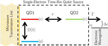
Figure 1: Color online. A schematic representation of the setup. A time-dependent driving field, $\Omega(t)$, in the microwave transmission line (left orange region) is coupled to QD1, a two-level quantum dot with ground level $\left|g\right>$ (blue line) and excited level $\left|e\right>$ (red line). QD1 is in turn tunnel coupled, with amplitude $\tau$, to QD2, a quantum dot with one level $\left|x\right>$ (green line) from which the electron may escape, with rate $\Gamma$, into the electronic waveguide (right gray region). The dashed rectangle shows the components of the single-electron time-bin qubit source.

Within quantum electronics, several types of single-electron sources (SES) are realized experimentally, for a review see Ref. Pekola et al. (2013), while electron emission using an optically driven double quantum dot has been proposed theoretically Stafford and Wingreen (1996), for a review see Ref. Platero and Aguado (2004), and recently also using circuit QED van den Berg et al. (2014). However, for an electronic flying qubit, controlling the electron phase is crucial. The earliest efforts to electrically control an electron phase in solid-state circuits required strong magnetic fields Washburn et al. (1987); de Vegvar et al. (1989); van Oudenaarden et al. (1998). The most recent demonstration combines an Aharonov-Bohm ring with a two-channel wire to generate solid-state flying qubits Yamamoto et al. (2012). The later setup is limited by backscattering at the ring-wire interface, resulting in a visibility of less than $1\%$. Here we propose a different approach, which allows to efficiently produce a highly controllable time-bin single-electron qubit. We suggest to employ a hybrid quantum system, see Fig. 1, where a microwave driving field is used to raise an electron from the ground state of a double quantum dot to the excited state above the Fermi level of a nearby electronic waveguide. The essential ingredient of our proposal is a controlled temporal dependence of the amplitude and phase of the driving field, that allows to produce the time-dependent amplitude and phase of an emitted electron. The experimental toolbox for such time-dependent manipulation of the microwave driving field was recently demonstrated for the amplitude Pechal et al. (2013); Wenner et al. (2013) and phase Hoi et al. (2013); Abdo et al. (2013); Tancredi et al. (2013).

To demonstrate coherence properties of single particles one may use one of several characterization schemes, e.g. Hanbury Brown–Twiss Brown and Twiss (1956a, b) (HBT), Mach–Zehnder Zehnder (1891); Mach (1892) (MZ), and Hong–Ou–Mandel Hong et al. (1987) (HOM) interferometry. These schemes were originally developed for optics, but have within the last two decades also been realized in electronics Henny et al. (1999); Oliver et al. (1999); Ji et al. (2003); Samuelsson et al. (2004); Neder et al. (2006, 2007); Samuelsson et al. (2009); Bocquillon et al. (2012); Dubois et al. (2013); Bocquillon et al. (2013); Dubois et al. (2013). The coherence properties of electrons emitted on-demand Fève et al. (2007); Dubois et al. (2013) were recently characterized via electronic Hong-Ou-Mandel interferometry Bocquillon et al. (2013); Dubois et al. (2013). These experiments demonstrate the possibility to achieve correlations between electrons emitted by independent sources and, for instance, open the opportunity to generate time-bin entangled electron pairs as suggested in Ref. Splettstoesser et al. (2009). Other recent proposals for such states utilize the helical edge states of a quantum spin Hall insulator Inhofer and Bercioux (2013); Hofer and Büttiker (2013).

In the following we first describe the setup and model of a source capable of creating SETBQs and then analyze its characterization using HOM interferometry.

Setup.— We consider a two-level quantum dot, QD1, tunnel coupled to a single-level quantum dot, QD2, which is coupled to an electronic waveguide, i.e. a ballistic conductor or an edge state, see Fig. 1. A microwave transmission line in the vicinity of QD1 allows the ground state, $\left|g\right>$, and exited state, $\left|e\right>$, to be coupled via a classical time-dependent microwave field, $\Omega(t)$. An electron in $\left|e\right>$ may tunnel with amplitude $\tau$ into the state $\left|x\right>$ of QD2 from which it can escape with rate $\Gamma$ into the electron waveguide at an energy state $\Delta\epsilon$ above the Fermi energy, $\epsilon_{F}$. The state $\left|x\right>$ of QD2 ensures that the electrons below the Fermi level of the electronic waveguide do not couple to QD1. While the analysis does not refer to a specific experimental setup, the scheme could be realized in a variety of systems such as by discrete levels of a carbon nanotube, where coupling to fermionic leads and a microwave circuit cavity has been realized Delbecq et al. (2011, 2013) or gate defined QDs coupled to microwave transmission lines as e.g. investigated in Refs. Frey et al. (2012a, b); Basset et al. (2013).

Model.— The Hamiltonian describing a quantum dot interacting with a microwave transmission line is well known Childress et al. (2004); Blais et al. (2004); Bergenfeldt and Samuelsson (2012). We assume an infinite on-site Coulomb interaction, such that the source is at most occupied by one electron, consider low temperature, such that no electrons leak from the electronic waveguide into the source, and treat the escape rate by a dissipative Lindblad term of state $\left|x\right>$. Thereby, in the interaction picture, the coherent evolution of a single electron in the source is described by the effective non-Hermitian Hamiltonian, ($\hbar=1$)

$$\mathcal{H}=(\Omega(t)\hat{a}^{\dagger}_{e}\hat{a}_{g}+\tau\hat{a}^{\dagger}_{e}\hat{a}_{x}+H.c.)-i\Gamma\hat{a}^{\dagger}_{x}\hat{a}_{x},$$ (1)

where the operators $\hat{a}_{i}$ and $\hat{a}^{\dagger}_{i}$ annihilate and create an electron in state $i$. For the time being we analyze the idealized situation and disregard decoherence effects from relaxation and dephasing for clarity, while we return to these important effects later.

In the basis of $\left|g\right>$, $\left|e\right>$, and $\left|x\right>$, this gives the Schrödinger equation

$$\frac{\partial}{\partial t}\left[\begin{array}[]{c}a_{g}\\ a_{e}\\ a_{x}\end{array}\right]=\left[\begin{array}[]{ccc}0&-i\Omega^{*}(t)&0\\ -i\Omega(t)&0&-i\tau\\ 0&-i\tau^{*}&-\Gamma\end{array}\right]\left[\begin{array}[]{c}a_{g}\\ a_{e}\\ a_{x}\end{array}\right].$$ (11)

The amplitudes $a_{i}$ of states $i=g,e,x$ are related to the density matrix elements $\rho_{ij}$ through $\rho_{ij}=a_{i}a_{j}^{*}$.

Equation (1) is identical to the effective Hamiltonian of the quantum optical analog for shaping a single photon envelope Law and Kimble (1997); Vasilev et al. (2010) described in the introduction. Specifically, our single-electron source is related to the driven $\Lambda$-type 3-level atom single-photon source, by mapping the microwave drive, $\Omega(t)$, the tunneling amplitude, $\tau$, and the escape rate, $\Gamma$, respectively to the optical drive, the atom-cavity coupling, and the cavity leakage. We may thus draw a parallel to the approach for photon shaping to design the single-electron wave packet.

Creating Single-Electron Time-Bin Qubits.— The electron that coherently escapes the source, propagates in the $z$-direction along the electronic waveguide with a single electron wave packet of the form $\Psi(t,z)=\psi(t,z)e^{i(\epsilon_{F}+\Delta\epsilon)t-ikz}$. Here, the envelope $\psi(t,z)$ is determined by the rate $\Gamma$ at which the population of the state $\left|x\right>$ decays, i.e. at $z_{S}$, the position of the source, $\psi$ is related to the density matrix element $\rho_{xx}(t)$ through $|\psi(t,z_{S})|^{2}=2\Gamma\rho_{xx}(t)$, and thereby, $a_{x}(t)=\psi(t,z_{S})/\sqrt{2\Gamma}$. In the following we omit the explicit dependence of $z$ for simplicity. Similar to the optical analog Vasilev et al. (2010), by solving Eq. (11) we can derive an equation, which determines the driving field, $\Omega(t)$, to be imposed in order to emit a specified single-electron envelope into an electronic waveguide. Furthermore, for time-bin qubits we find that the time-dependent phase of $\Omega(t)$ directly transfers to the phase of the envelope.

From the derivation of $\Omega(t)$, the shape of the envelope is limited by

$$|\psi(t)|^{2}\leq 2\Gamma,\quad\mbox{and}\quad|\partial_{t}\psi(t)+\Gamma\psi(t)|^{2}\leq 2\Gamma|\tau|^{2}.$$ (12)

These inequalities physically signify that the temporal variation of the envelope cannot be faster than the internal timescales of the source. Specifically, the first inequality results in a limit to the width, $T$, of the envelope as a result of the finite escape rate, $\Gamma$. The second inequality shows that the temporal variation of the envelope is limited by the tunneling rate between the two dots in combination with the escape rate. Moreover, as it is known from the optical analog Vasilev et al. (2010), the coupling between the driving field and a QD depends on the occupancy of the QD. Thus, since the occupancy of QD1 decreases during the emission process, the amplitude of the driving field has to be increasingly strong to fully emit the single electron. Therefore, in practice, the electron is partially emitted. To account for this effect we introduce the efficiency of the source, $\eta$, and represent $\psi=\sqrt{\eta}\psi_{0}$, with the efficiency $0<\eta<1$ and the ideal envelope $\psi_{0}$ having unit time integral. These features are best illustrated by an example.

We consider the emission of a time-binned single electron with an envelope $\psi_{0}(t)=\psi_{sp}(t,0)+\psi_{sp}(t,T/2)e^{i\varphi}$ where $\psi_{sp}(t,t^{\prime})$ is a semi-pulse given

$$\psi_{sp}(t,t^{\prime})=\frac{4}{\sqrt{5T}}\sin^{3}\left(\frac{2\pi t}{T}\right),\qquad t^{\prime}\leq t\leq\frac{T}{2}+t^{\prime}.$$ (13)

This gives a time-bin qubit of the form $\left|\psi\right>=\frac{1}{\sqrt{2}}(\left|10\right>+e^{i\varphi}\left|01\right>)$, where e.g. $\left|10\right>$ represents an electron in the first semi-pulse. The envelope is shown in the inset of Fig. 2. For $\tau=2\Gamma$ and $T=100/G$ the temporal shape of the needed field amplitude, $|\Omega(t)|$, is shown in Fig. 2 for different $\eta$. The temporal shape of the first part of $\Omega(t)$ only changes slightly when increasing $\eta$, while the second part on the other hand has to be increasingly skewed due to the reduced occupancy of QD1.

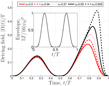
Figure 2: Color online. The calculated temporal shape of the drive $|\Omega(t)|/\Gamma$ in order to obtain the single-electron TBQ, Eq. (13), for different $\eta$. The parameters used for the source are $\tau=2\Gamma$ and $T=100/\Gamma$. Inset: The squared envelope of an emitted electron normalized in maximum to unity.

We have thus presented a source capable of emitting time-bin qubits. We notice that, even though we have focused on such single electron envelopes, the scheme is not limited to these. In fact any single electron envelope shape is allowed, only restricted by the internal timescales of the source through inequalities Eq. (12).

Characterization.— Having described a source for creating SETBQs, we next analyze a possible way of characterizing it, specifically using the HOM scheme. The HOM scheme, shown in the inset of Fig. 3, consists of a beam-splitter (BS) having two input ports, 1 and 2, and two output ports, 3 and 4. Electrons are emitted into the input ports followed by the zero-frequency current correlations measurement of the output ports, i.e. Blanter and Büttiker (2000)

$$S_{34} =\iint\mathrm{d}t\mathrm{d}t^{\prime}[\left<\hat{n}_{3}(t)\hat{n}_{4}(t^{\prime})\right>-\left<\hat{n}_{3}(t)\right>\left<\hat{n}_{4}(t^{\prime})\right>],$$ (14)

where $\hat{n}_{\alpha}(t)$ is the current flux operator of channel $\alpha$. If only one of the sources, S1 or S2, is active we get the HBT correlations, $S^{HBT}_{S1}$ or $S^{HBT}_{S2}$, which are identical for identical sources, $S^{HBT}_{S1}=S^{HBT}_{S2}=S^{HBT}$. If both sources are active, the HOM correlations, $S^{HOM}$, are measured and one may define the HOM correlations normalized with respect to the HBT correlations, $\mathcal{S}_{34}=S^{HOM}_{34}/(2S^{HBT})$, to get a quantity which is independent of the transmission and reflection probabilities of the BS and, furthermore, to reduce the effect of temperature Bocquillon et al. (2013). Assuming that none of the energy components of the envelopes overlap with the Fermi sea, we have that Jonckheere et al. (2012)

$$\mathcal{S}_{34} =1-\left|\int\mathrm{d}t\;\psi_{1}^{*}(t)\psi_{2}(t)\right|^{2}.$$ (15)

In Fig. 3 we show $\mathcal{S}_{34}$ calculated for two sources, S1 and S2, emitting single electrons with envelopes $\psi_{1}$ and $\psi_{2}$ of the form in Eq. (13) and partial phases $\varphi_{1}$ and $\varphi_{2}$, respectively, with $\delta\varphi=\varphi_{2}-\varphi_{1}$. The sources S1 and S2 are synchronized such that emitted electrons arrive at the beam splitter with a time delay $\delta t$.

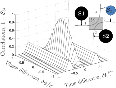
Figure 3: The HOM correlations vs phase difference, $\delta\varphi$, and time difference, $\delta t$. Parameters used are $\tau=2\Gamma$, a desired envelope of width $T=100/\Gamma$, and source efficiency $\eta=0.99$. For $\Omega(t)$, see the solid black line in Fig. 2. Inset: Sketch of the HOM setup. The two sources S1 and S2 emit single electrons, which collide at the beam splitter BS and the current correlations, $\mathcal{S}_{34}$, between the arms 3 and 4 are measured.

First, for $\delta t=0$, we have $\mathcal{S}_{34}=1-\eta^{2}\cos^{2}(\delta\varphi/2)$ and thus for $\delta\varphi=0$, corresponding to two identical incident single-electron envelopes, the current correlation is $\mathcal{S}_{34}=1-\eta^{2}$. For unit efficiency, $\eta=1$, each electron incoming from the port $1$ encounters an electron incoming from the port $2$. At $\delta t=0$, the perfect overlap of the envelopes results in $\mathcal{S}_{34}=0$, i.e. the electrons are scattered into different output ports $3$ and $4$. This anti-bunching is known as the Pauli peak and reflects the fermionic nature such that two electrons cannot occupy the same state at the same time Blanter and Büttiker (2000); Ol’khovskaya et al. (2008). The Pauli peak can be seen in Fig. 3 at $\delta\varphi=0$ close to $\delta t=0$.

As $\delta\varphi$ changes from zero to $\pi$ we observe that, interestingly, the Pauli peak at $\delta t=0$ disappears. That is, even though the two electrons arrive at exactly the same time, such that $|\psi_{1}(t)|=|\psi_{2}(t)|$, they seemingly do not obey the Pauli principle. This peculiar observation is caused by the two envelopes at $\delta\varphi=\pi$ being orthogonal to each other and thus do not constitute the same states, i.e. their overlap is zero and electrons can be scattered to the same output port. At equal arrival time, the difference between $\mathcal{S}_{34}$ for $\delta\varphi=0$ and $\delta\varphi=\pi$ shows the difference between the two states $\left|\psi\right>=\frac{1}{\sqrt{2}}(\left|10\right>\pm\left|01\right>)$ and thus $\mathcal{S}_{34}$ constitutes the source visibility.

Lastly, by changing the time-delay, $\delta t$, two phase-independent smaller peaks are seen at $\delta t=\pm T/2$. These correspond to the overlap of the front pulse of $\psi_{1}(t)$ with the tail pulse of $\psi_{2}(t)$ and vice versa. We have thus shown that, by varying the time-delay, $\delta t$, and phase difference, $\delta\varphi$, between the two SETBQ, we are able to characterize our proposed source using the HOM scheme.

Decoherence Effects.— Until now we have neglected the important issues of the relaxation of QD1 and dephasing due to the tunneling between QD1 and QD2. Since we are interested in the coherent evolution of the electron, we follow Ref. Vasilev et al. (2010) and describe the decoherence by a dissipation of the coherent electron to derive an effective Hamiltonian as used in the quantum-jump approach to dissipative systems known from quantum optics, see e.g. Refs. Zoller et al. (1987); Carmichael (1993); Plenio and Knight (1998). This is done by including a relaxation rate $\gamma_{r}$ of state $\left|e\right>$ and tunneling dephasing rate $\gamma_{\phi}$ of states $\left|e\right>$ and $\left|x\right>$ as dissipations in the effective Hamiltonian, Eq. (1), governing the coherent electron. This implicitly assumes that a photon emitted into the microwave transmission line due to the relaxation of QD1, does not reexcite the QD. We may then again derive an equation, which determines $\Omega(t)$ for the coherent emission of a specified single electron envelope into the electronic waveguide. From the conservation of charge one finds that the decoherence terms lead to the physical limit on the maximal efficiency, similar to the optical analog Vasilev et al. (2010),

$$\eta_{\max}=\frac{1}{1+\frac{(\gamma_{r}+\gamma_{\phi})}{\Gamma|\tau|^{2}}\left[\Gamma^{2}+\int_{0}^{T}\mathrm{d}t^{\prime}|\partial_{t^{\prime}}\psi_{0}(t^{\prime})|^{2}\right]+\frac{\gamma_{\phi}}{\Gamma}},$$ (16)

i.e. the efficiency has to be in the interval $0\leq\eta\leq\eta_{\max}$. The case $\eta=\eta_{\max}<1$ signifies that the decoherence results in the emitted electron being in a statistical mixture of being coherently emitted with probability $\eta$ and incoherently emitted with probability $1-\eta$. To give an estimate of $\eta_{\max}$ we take the currently achievable experimental values $\tau/(2\pi)\sim 15.5$GHz, $\gamma_{r}/(2\pi)\sim 100$MHz, and $\gamma_{\phi}/(2\pi)\sim 1.5$GHz from Ref. Basset et al. (2013) and $\Gamma\sim\tau/2$ from Frey et al. (2012b) and $T=100/G$ as used in Figs. 2 and 3 giving $\eta_{\max}\sim 0.8$ for the SETBQ, Eq. (13). This suggests that, with current technology, our proposed source has the possibility of a significantly increased efficiency compared to state-of-the-art flying qubit sources Yamamoto et al. (2012).

Reloading the Source.— Lastly, let us describe three possible methods for reloading the source for gate defined QDs. First, a laser pulse could excite electrons from the buffer layer to the state $\left|g\right>$ as experimentally demonstrated in Ref. Fujita et al. (2013) and thereby deterministically load the source with a new electron on demand. A second method is to tune the voltage gates to lower the energy level of state $\left|x\right>$ below the Fermi sea of the electronic waveguide to the level of $\left|g\right>$. This would permit an electron (only one due to the Coulomb energy) to stochastically flow from the electronic waveguide into $\left|x\right>$ and then tunnel back and forth between $\left|g\right>$ and $\left|x\right>$. Since it is below the Fermi sea it would not decay back into the electronic waveguide. Then if $\left|x\right>$ is slowly raised, the electron would end in $\left|g\right>$. A third option is to couple QD1 very weakly to an electron reservoir. If the time scale of the electron tunneling from the reservoir to QD1 is much longer than the electron emission time of the source, then there would only be a minimal risk of having more than one electron in the emitted electron time-bin.

Summary and Outlook.— We proposed a single-electron source relying on a hybrid quantum system. With our scheme one can design an electron envelope thereby providing control over the phase and the amplitude of a single electron. In particular, we analyzed the emission of a single-electron time-bit qubit, and showed how to characterize it using a well-known interferometric technique. Specifically, we showed that in Hong–Ou–Mandel interferometry the Pauli peak can be continuously removed by controlling the phase difference of two time-bin qubits. Our analysis showed that, with experimentally relevant parameters, the source efficiency is expected to be close to unity. This opens the possibility of using single electrons for quantum operations in scalable solid-state architectures. Furthermore, with the recent demonstration of creating single microwave photons with controlled envelopes Pechal et al. (2013); Wenner et al. (2013) our proposed scheme constitutes a possible photon-electron interface for photon-to-electron time-bin qubit conversion with microwave coupling in the vacuum Rabi regime.

Acknowledgment.— We are most grateful to Markus Büttiker who raised the problem addressed here and participated in the initial stage of this work. Markus sadly passed away before the project was finalized. We thank D. Dasenbrook, P. P. Hofer, C. Flindt, P. Samuelsson, and M. Wubs for comments to the manuscript. JRO acknowledges financial support from the Danish Council of Independent Research. Research in Geneva is supported by the Swiss NSF.

References

- Nielsen and Chuang (2000) M. A. Nielsen and I. L. Chuang, Quantum Computation and Quantum Information, 1st ed. (Cambridge University Press, Cambridge, 2000).
- Wallraff et al. (2004) A. Wallraff, D. I. Schuster, A. Blais, L. Frunzio, R.-S. Huang, J. Majer, S. Kumar, S. M. Girvin, and R. J. Schoelkopf, Nature 431, 162 (2004).
- Schoelkopf and Girvin (2008) R. J. Schoelkopf and S. M. Girvin, Nature 451, 664 (2008).
- Franceschi et al. (2010) S. D. Franceschi, L. Kouwenhoven, C. Schönenberger, and W. Wernsdorfer, Nature Nanotechnology 5, 703 (2010).
- You and Nori (2011) J. Q. You and F. Nori, Nature 474, 589 (2011).
- Delbecq et al. (2011) M. R. Delbecq, V. Schmitt, F. D. Parmentier, N. Roch, J. J. Viennot, G. Fève, B. Huard, C. Mora, A. Cottet, and T. Kontos, Phys. Rev. Lett. 107, 256804 (2011).
- Frey et al. (2012a) T. Frey, P. J. Leek, M. Beck, A. Blais, T. Ihn, K. Ensslin, and A. Wallraff, Phys. Rev. Lett. 108, 046807 (2012a).
- Frey et al. (2012b) T. Frey, P. J. Leek, M. Beck, J. Faist, A. Wallraff, K. Ensslin, T. Ihn, and M. Büttiker, Phys. Rev. B 86, 115303 (2012b).
- Petersson et al. (2012) K. D. Petersson, L. W. McFaul, M. D. Schroer, M. Jung, J. M. Taylor, A. A. Houck, and J. R. Petta, Nature 490, 380 (2012).
- Basset et al. (2013) J. Basset, D.-D. Jarausch, A. Stockklauser, T. Frey, C. Reichl, W. Wegscheider, T. M. Ihn, K. Ensslin, and A. Wallraff, Phys. Rev. B 88, 125312 (2013).
- Delbecq et al. (2013) M. Delbecq, L. Bruhat, J. Viennot, S. Datta, A. Cottet, and T. Kontos, Nature Communs. 4, 1400 (2013).
- van Loo et al. (2013) A. F. van Loo, A. Fedorov, K. Lalumière, B. C. Sanders, A. Blais, and A. Wallraff, Science 342, 1494 (2013).
- Toida et al. (2013) H. Toida, T. Nakajima, and S. Komiyama, Phys. Rev. Lett. 110, 066802 (2013).
- Viennot et al. (2013) J. Viennot, M. Delbecq, M. Dartiailh, A. Cottet, and T. Kontos, arXiv:1310.4363v1 (2013).
- Deng et al. (2013) G.-W. Deng, D. Wei, J. Johansson, M.-L. Zhang, S.-X. Li, H.-O. Li, G. Cao, M. Xiao, T. Tu, G.-C. Guo, H.-W. Jiang, F. Nori, and G.-P. Guo, arXiv:1310.6118v1 (2013).
- Liu et al. (2014) Y.-Y. Liu, K. D. Petersson, J. Stehlik, J. M. Taylor, and J. R. Petta, arXiv:1401.7730v1 (2014).
- Law and Kimble (1997) C. K. Law and H. J. Kimble, J. Mod. Opt 44, 2067 (1997).
- Keller et al. (2004a) M. Keller, B. Lange, K. Hayasaka, W. Lange, and H. Walther, New J. Phys. 6, 95 (2004a).
- Vasilev et al. (2010) G. S. Vasilev, D. Ljunggren, and A. Kuhn, New J. Phys. 12, 063024 (2010).
- Kuhn et al. (2002) A. Kuhn, M. Hennrich, and G. Rempe, Phys. Rev. Lett. 89, 067901 (2002).
- Keller et al. (2004b) M. Keller, B. Lange, K. Hayasaka, W. Lange, and H. Walther, Nature Physics 431, 1075 (2004b).
- Nisbet-Jones et al. (2011) P. B. R. Nisbet-Jones, J. Dilley, D. Ljunggren, and A. Kuhn, New J. Phys. 13, 103036 (2011).
- Nisbet-Jones et al. (2013) P. B. R. Nisbet-Jones, J. Dilley, A. Holleczek, O. Barter, and A. Kuhn, New J. Phys. 15, 053007 (2013).
- Matthiesen et al. (2013) C. Matthiesen, M. Geller, C. H. H. Schulte, C. L. Gall, J. Hansom, Z. Li, M. Hugues, E. Clarke, and M. Atatüre, Nature Comms. 4, 2601 (2013).
- Pechal et al. (2013) M. Pechal, C. Eichler, S. Zeytinoglu, S. Berger, A. Wallraff, and S. Filipp, ArXiv:1308.4094v1 (2013).
- Wenner et al. (2013) J. Wenner, Y. Yin, Y. Chen, R. Barends, B. Chiaro, E. Jeffrey, J. Kelly, A. Megrant, J. Y. Mutus, C. Neill, P. J. J. O’Malley, P. Roushan, D. Sank, A. Vainsencher, T. C. White, A. N. Korotkov, A. N. Cleland, and J. M. Martinis, arXiv:1311.1180v2 (2013).
- Pekola et al. (2013) J. P. Pekola, O.-P. Saira, V. F. Maisi, A. Kemppinen, M. Möttönen, Y. A. Pashkin, and D. V. Averin, Rev. Mod. Phys. 85, 1421 (2013).
- Stafford and Wingreen (1996) C. A. Stafford and N. S. Wingreen, Phys. Rev. Lett. 76, 1916 (1996).
- Platero and Aguado (2004) G. Platero and R. Aguado, Phys. Rep. 395, 1 (2004).
- van den Berg et al. (2014) T. L. van den Berg, C. Bergenfeldt, and P. Samuelsson, arXiv:1402.1351v1 (2014).
- Washburn et al. (1987) S. Washburn, H. Schmid, D. Kern, and R. A. Webb, Phys. Rev. Lett. 59, 1791 (1987).
- de Vegvar et al. (1989) P. de Vegvar, G. Timp, P. Mankiewich, R. Behringer, and J. Cunningham, Phys. Rev. B 40, 3491 (1989).
- van Oudenaarden et al. (1998) A. van Oudenaarden, M. H. Devoret, Y. V. Nazarov, and J. E. Mooij, Nature 391, 768 (1998).
- Yamamoto et al. (2012) M. Yamamoto, S. Takada, C. Baüerle, K. Watanabe, A. D. Wieck, and S. Tarucha, Nature Nanotechnology 7, 247 (2012).
- Hoi et al. (2013) I.-C. Hoi, A. F. Kockum, T. Palomaki, T. M. Stace, B. Fan, L. Tornberg, S. R. Sathyamoorthy, G. Johansson, P. Delsing, and C. M. Wilson, Phys. Rev. Lett. 111, 053601 (2013).
- Abdo et al. (2013) B. Abdo, K. Sliwa, F. Schackert, N. Bergeal, M. Hatridge, L. Frunzio, A. D. Stone, and M. Devoret, Phys. Rev. Lett. 110, 173902 (2013).
- Tancredi et al. (2013) G. Tancredi, G. Ithier, and P. J. Meeson, Appl. Phys. Lett. 103, 063504 (2013).
- Brown and Twiss (1956a) R. H. Brown and R. Q. Twiss, Nature 177, 27 (1956a).
- Brown and Twiss (1956b) R. H. Brown and R. Q. Twiss, Nature 178, 1447 (1956b).
- Zehnder (1891) L. Zehnder, Zeitschrift für Instrumentenkunde 11, 275 (1891).
- Mach (1892) L. Mach, Zeitschrift für Instrumentenkunde 12, 89 (1892).
- Hong et al. (1987) C. K. Hong, Z. Y. Ou, and L. Mandel, Phys. Rev. Lett. 59, 2044 (1987).
- Henny et al. (1999) M. Henny, S. Oberholzer, C. Strunk, T. Heinzel, K. Ensslin, M. Holland, and C. Schönenberger, Science 284, 296 (1999).
- Oliver et al. (1999) W. D. Oliver, J. Kim, R. C. Liu, and Y. Yamamoto, Science 284, 299 (1999).
- Ji et al. (2003) Y. Ji, Y. Chung, D. Sprinzak, M. Heiblum, D. Mahalu, and H. Shtrikman, Nature 422, 415 (2003).
- Samuelsson et al. (2004) P. Samuelsson, E. V. Sukhorukov, and M. Büttiker, Phys. Rev. Lett. 92, 026805 (2004).
- Neder et al. (2006) I. Neder, M. Heiblum, Y. Levinson, D. Mahalu, and V. Umansky, Phys. Rev. Lett. 96, 016804 (2006).
- Neder et al. (2007) I. Neder, N. Ofek, Y. Chung, M. Heiblum, D. Mahalu, and V. Umansky, Nature 448, 333 (2007).
- Samuelsson et al. (2009) P. Samuelsson, I. Neder, and M. Büttiker, Phys. Rev. Lett. 102, 106804 (2009).
- Bocquillon et al. (2012) E. Bocquillon, F. D. Parmentier, C. Grenier, J.-M. Berroir, P. Degiovanni, D. C. Glattli, B. Plaçais, A. Cavanna, Y. Jin, and G. Fève, Phys. Rev. Lett. 108, 196803 (2012).
- Dubois et al. (2013) J. Dubois, T. Jullien, F. Portier, P. Roche, A. Cavanna, Y. Jin, W. Wegscheider, P. Roulleau, and D. C. Glattli, Nature 502, 659 (2013).
- Bocquillon et al. (2013) E. Bocquillon, V. Freulon, J.-M. Berroir, P. Degiovanni, B. Plaçais, A. Cavanna, Y. Jin, and G. Fève, Science 339, 1054 (2013).
- Fève et al. (2007) G. Fève, A. Mahé, J.-M. Berroir, T. Kontos, B. Plaçais, D. C. Glattli, A. Cavanna, B. Etienne, and Y. Jin, Science 316, 1169 (2007).
- Splettstoesser et al. (2009) J. Splettstoesser, M. Moskalets, and M. Büttiker, Phys. Rev. Lett. 103, 076804 (2009).
- Inhofer and Bercioux (2013) A. Inhofer and D. Bercioux, Phys. Rev. B 88, 235412 (2013).
- Hofer and Büttiker (2013) P. P. Hofer and M. Büttiker, Phys. Rev. B 88, 241308(R) (2013).
- Childress et al. (2004) L. Childress, A. S. Sørensen, and M. D. Lukin, Phys. Rev. A 69, 042302 (2004).
- Blais et al. (2004) A. Blais, R.-S. Huang, A. Wallraff, S. M. Girvin, and R. J. Schoelkopf, Phys. Rev. A 69, 062320 (2004).
- Bergenfeldt and Samuelsson (2012) C. Bergenfeldt and P. Samuelsson, Phys. Rev. B 85, 045446 (2012).
- Blanter and Büttiker (2000) Y. M. Blanter and M. Büttiker, Phys. Rep. 336, 1 (2000).
- Jonckheere et al. (2012) T. Jonckheere, J. Rech, C. Wahl, and T. Martin, Phys. Rev. B 86, 125425 (2012).
- Ol’khovskaya et al. (2008) S. Ol’khovskaya, J. Splettstoesser, M. Moskalets, and M. Büttiker, Phys. Rev. Lett. 101, 166802 (2008).
- Zoller et al. (1987) P. Zoller, M. Marte, and D. F. Walls, Phys. Rev. A 35, 198 (1987).
- Carmichael (1993) H. Carmichael, An Open Systems Approach to Quantum Optics (Springer, Berlin, 1993).
- Plenio and Knight (1998) M. B. Plenio and P. L. Knight, Rev. Mod. Phys. 70, 101 (1998).
- Fujita et al. (2013) T. Fujita, H. Kiyama, K. Morimoto, S. Teraoka, G. Allison, A. Ludwig, A. D. Wieck, A. Oiwa, and S. Tarucha, Phys. Rev. Lett. 110, 266803 (2013).