Relaxation in Luttinger liquids: Bose-Fermi duality

Abstract

We explore the life time of excitations in a dispersive Luttinger liquid. We perform a bosonization supplemented by a sequence of unitary transformations that allows us to treat the problem in terms of weakly interacting quasiparticles. The relaxation described by the resulting Hamiltonian is analyzed by bosonic and (after a refermionization) by fermionic perturbation theory. We show that the the fermionic and bosonic formulations of the problem exhibit a remarkable strong-weak-coupling duality. Specifically, the fermionic theory is characterized by a dimensionless coupling constant $\lambda=m^{*}l^{2}T$ and the bosonic theory by $\lambda^{-1}$, where $1/m^{*}$ and $l$ characterize the curvature of the fermionic and bosonic spectra, respectively, and $T$ is the temperature.

I Introduction

Quantum kinetics in interacting one-dimensional (1D) systems is a subject of an active experimental and theoretical investigation. There is a variety of experimental realizations of 1D fermionic systems which include, in particular, carbon nanotubes, semiconductor and metallic nanowires, as well as edge states of quantum Hall systems and of other 2D topological insulator structures. Further, cold atomic gases in optical traps can be used to engineer 1D fermionic or bosonic systems with a tunable interaction. A light or microwaves in waveguides with interaction mediated by two-level systems represent another realization of a correlated 1D bosonic system.

A common and very powerful theoretical approach to interacting 1D systems is the bosonization Stone_book ; Delft ; Gogolin ; Giamarchi . When the spectral curvature and backscattering processes are neglected, bosonization maps the problem of interacting fermions (known as Tomonaga-Luttinger model) to the Luttinger liquid theory of free bosons (plasmons). A mapping to the Luttinger liquid is also obtained if one starts from the problem of bosons with repulsion. If the interaction is considered as momentum-independent (i.e. local in the coordinate space), the spectrum of Luttinger-liquid bosonic excitations is linear, and by virtue of refermionization the problem is equivalent to that of free fermions. In brief, when the momentum dispersions of excitations are neglected, the fermionic and bosonic 1D problems are equivalent, and the interaction can be completely eliminated.

The problem becomes much more complex when both the spectral curvature of constituent particles and the momentum dependence of the interaction are retained. This leads (apart from some special cases) to a violation of integrability of the theory. While the corresponding corrections to the Luttinger liquid theory are irrelevant in the renormalization-group (RG) sense, they are very important from the physical point of view. Specifically, they establish a finite relaxation rate of excitations when the system is at non-zero temperature or away from equilibrium.

Several recent works addressed various aspects of relaxation in 1D problems. In Refs. Lunde07, ; Khodas2007, ; imambekov09, ; imambekov11, a perturbative analysis of three-particle scattering in a model of weakly interacting fermions with a spectral curvature (inverse mass) $m^{-1}$ was performed. It was found, in particular, that in the case of spinless fermions the intrabranch scattering processes (RRL $\to$ RRL and RLL $\to$ RLL, where R and L denote right- and left-movers, respectively) induce a scattering rate of an excitation with momentum $k$ that scales as $(k-k_{F})^{8}/m^{3}$ at zero temperature and $(k-k_{F})^{6}T/m^{2}$ at sufficiently high temperature $T$, where $k_{F}$ is the Fermi momentum. These results were generalized to the case of Coulomb interaction in Refs. micklitz11, ; ristivojevic13, .

The opposite limiting case of Luttinger liquid with interaction parameter $K\ll 1$ (describing, in particular, fermions with very strong repulsive interaction, when the system can be viewed as “almost a Wigner crystal”) was considered in Refs. apostolov13, ; Lin2013, . The authors of these works analyzed the decay rate of bosonic excitations in such systems and found the decay rate scaling as $T^{5}$.

The goal of this work is to study systematically relaxation in dispersive Luttinger liquids in the whole space of parameters. We start from the interacting fermionic problem, then bosonize it and perform a unitary transformation PGM2013 (that extends the one originally introduced in Ref. Matis_Lieb1965, ; see also Refs. Rozhkov, ; imambekov11, ; MatveevFurusaki2013, ) which allows one to eliminate a major part of the interaction. In particular, in this way the two chiral branches get decoupled up to the third order in density fluctuations. In Ref. PGM2013, this formalism was employed to develop a formalism of kinetic equation for fermionic quasiparticles. A focus in that work was on a not too long time scale where the collisions between quasiparticles can be neglected. Here we use the theory resulting from the above unitary transformation to find the relaxation rate of excitations. We perform both fermionic and bosonic analysis of this theory, evaluate the corresponding relaxation rates, and determine regions of the parameter space where each of the approaches is applicable. This allows us to establish a remarkable picture of Fermi-Bose duality in dispersive interacting 1D systems.

The structure of this article is as follows. In Sec. II we introduce a model of a generic dispersive Luttinger liquid in terms of fermions with a spectral curvature $1/m$ and an interaction with an arbitrary strength and a radius $l_{\rm int}$. The fact that both parameters $1/m$ and $l_{\rm int}$ are non-zero makes the problem non-integrable. We perform a bosonization of this model supplemented by a unitary transformation that maps it onto a problem of weakly interacting bosonic quasiparticles. In Sec. III we calculate the lifetime of bosonic excitations within this theory. In Sec. IV we refermionize the theory obtained in Sec. II and explore the relaxation of fermionic excitations. For this purpose, we calculate the contributions to this relaxation rate from both inter-branch and intra-branch scattering processes. Finally, in Sec. V we collect and analyze the obtained results and determine the behavior of the relaxation rate in the whole parameter space. We show that the parameter space is subdivided in the “fermionic” and “bosonic” domains with a dimensionless control parameter $m^{*}l^{2}T$, where the effective mass $m^{*}$ and the plasmon dispersion length $l$ are expressed in terms of the bare parameters $m$, $l_{\rm int}$ and the Luttinger-liquid constant $K_{0}$. The emerging picture has a character of Fermi-Bose weak-strong coupling duality. We close the paper by summarizing our results and discussing prospects for future research in Sec. VI.

II Dispersive Luttinger liquids

In this section we introduce the Hamiltonian of our model and formulate basic questions to be addressed in the paper. We then perform a sequence of unitary transformations bringing the theory to a form amenable to a perturbative treatment and highlighting the duality between fermionic and bosonic descriptions of the dispersive Luttinger liquids.

II.1 The model

Our starting point is the Hamiltonian of a generic “dispersive” Luttinger liquid comprised of (spinless) right- and left-moving fermions (created and annihilated by operators $\psi^{+}_{\eta}(x)$, $\psi_{\eta}(x)$ with $\eta=R,L$; occasionally, we also use the notation $\eta=\pm 1$) with curved single-particle spectrum $\epsilon_{\eta}(k)=\eta kv_{F}+k^{2}/2m$ interacting via a generic finite-range density-density interaction $g(x)$

$$H=\sum_{\eta}\int dx\psi^{+}_{\eta}(x)\left(-i\eta v_{F}\partial_{x}-\frac{1}{2m}\partial_{x}^{2}\right)\psi_{\eta}(x)\\ +\frac{1}{2}\int dxdx^{\prime}g(x-x^{\prime})\rho(x)\rho(x^{\prime})\,.$$ (1)

Here $\rho(x)=\rho_{R}(x)+\rho_{L}(x)$. We characterize the interaction $g(x)$ by its strength at zero momentum $g_{0}$ and its radius $l_{\mathrm{int}}\gtrsim 1/(mv_{F})$ so that in momentum space

$$g_{q}=g_{0}\left(1-q^{2}l_{\mathrm{int}}^{2}\right)\,,\qquad ql_{\mathrm{int}}\ll 1\,.$$ (2)

We are interested in the properties of our model at low momenta $q\ll l_{\mathrm{i}nt}\lesssim p_{F}\equiv mv_{F}$ and energies $\epsilon\ll p_{F}v_{F}$.

In the subsequent consideration we will neglect the processes changing the total number of fermions $N_{\eta}$ (counted from its value in the ground state) within each chiral branch. They are absent in our model Hamiltonian (1) but are of course present in any real 1D system. These processes play a crucial role in the ultimate equilibration between branches in the Luttinger liquid Lunde07 ; Matveev2013 ; Dmitriev2012 but show up only at exponentially large time scales $\propto\exp(E_{F}/T)$ and are completely irrelevant for the physics discussed in this work. Accordingly, from now on we consider our system in the sector characterized by $N_{R}=N_{L}=0$ and set the zero Fourier components of the densities $\rho_{\eta}(x)$ to zero.

The standard Tomonaga-Luttinger (TL) is the extreme low-energy limit of the Hamiltonian (1) corresponding to linear fermionic spectrum ($m=\infty$) and point-like interaction $g(x)=g_{0}\delta(x)$. From the RG perspective, contributions that are neglected within this approximation are irrelevant perturbations. Specifically, when setting $m=\infty$, one drops an irrelevant perturbation of scaling dimension $3$, while discarding the momentum dependence of the interaction is equivalent [for a finite-range $g(x)$] to the neglect of even weaker perturbation of scaling dimension $4$. The bosonization approach Stone_book ; Delft ; Giamarchi ; Gogolin allows one to map the TL Hamiltonian onto free dispersionless bosons, which in turn are equivalent via refermionazation Matis_Lieb1965 ; Rozhkov ; imambekov09 ; imambekov11 to free fermions. Thus, the TL model can be equally well treated in bosonic and fermionic (after the identification of the proper fermionic modes) languages. This fact is related to the conformal invariance of the TL Hamiltonian.

Despite the great success of the TL model in the description of thermodynamic properties of 1D interacting fermions, it is now known that the irrelevant perturbations it neglects can have strong impact on the dynamical response of the system. For example, the fermionic curvature translates upon bosonization into a cubic interaction of the density fluctuationsschick68

$$-\frac{1}{2m}\int dx\psi^{+}_{\eta}(x)\partial_{x}^{2}\psi_{\eta}(x)\\ =\frac{2\pi^{2}}{3m}\int dx\rho_{\eta}^{3}(x)\,.$$ (3)

Although irrelevant in the RG sense, this perturbation acts for the case of a short-range interaction $g(x)$ (or just for free fermions), on a highly degenerate linear bosonic spectrum, so that the corresponding perturbation theory suffers from strong divergences. As a consequence, the formally irrelevant perturbation alters dramatically the behavior of, e.g., single particle spectral weight $A(k,\epsilon)$ in the immediate vicinity of the single-particle mass shellimambekov09 ; imambekov11 .

While extremely nontrivial in the bosonic representation, the problem of Luttinger liquid with finite fermionic mass can be elegantly addressed via the introduction of the proper fermionic quasiparticles (refermionization) Rozhkov ; imambekov09 ; imambekov11 . Thus the fermionic curvature breaks the symmetry between fermionic and bosonic languages present in the TL model in favor of fermions.

Conversely, for fermions with linear spectrum ($m=\infty$) the Hamiltonian (1) describes (after bosonization) free bosons with the dispersion relation

$$\omega_{q}=u_{q}|q|\,,\qquad u_{q}=v_{F}\left(1+\frac{g_{q}}{\pi v_{F}}\right)^{1/2}\equiv\frac{v_{F}}{K_{q}}\,.$$ (4)

At small momenta the boson velocity $u_{q}$ is given by

$$u_{q}=u_{0}\left(1-l^{2}q^{2}\right)\,,$$ (5)

$$l^{2}=\frac{1}{2}(1-K_{0}^{2})l_{\mathrm{int}}^{2}\,,$$ (6)

where $K_{0}$ is the zero-momentum limit of the Luttinger-liquid parameter $K_{q}$ introduced in Eq. (4). Finite interaction radius $l_{\mathrm{int}}$ leads thus to the appearance of dispersion in the bosonic spectrum. For long-range interactions the Wigner-crystal-type correlations proliferate and bosonic excitations are stable against perturbations caused by the curvature of fermionic spectrumLin2013 in a wide range of energies. Note that upon refermionization, the curvature of bosonic spectrum translates into an interaction between fermionic quasiparticles imambekov09 ; PGM2013 .

The consideration just presented raises the fundamental question: What are the proper degrees of freedom for the description of a generic dispersive Luttinger liquid having both curved fermionic and bosonic spectra? We observe a remarkable duality between the fermionic and bosonic description of the problem: curved single-particle spectrum for the excitations of one type (fermions or bosons) introduces the interaction between the excitations of the other type. The importance of this interaction for the dynamics of the particles of the second type is determined in turn by the curvature of their own spectrum. Accordingly, we expect that in a generic dispersive Luttinger liquid the particles with the most curved spectrum are the most long-living and well defined excitations. For a finite-range interaction $g(x)$, the nonlinear corrections to the bosonic and fermionic excitation spectra scale differently with momentum. Specifically, at sufficiently large momenta the bosonic correction $\delta\omega_{q}\propto v_{F}l_{\rm int}^{2}q^{3}$ dominates over the fermionic correction $\delta\xi_{k}\propto k^{2}/m$, while at small momenta the situation is reverse. Thus, one can expect that if the characteristic energy scale of the problem (say, temperature $T$) exceeds $T_{0}\propto 1/ml_{\rm int}^{2}$, the bosonic language gives the proper description of relaxation in the system, while at smaller energies the fermionic language becomes appropriate.

In the rest of the paper we explore the life time of bosonic and fermionic excitations in the dispersive Luttinger liquid. To be definite, we consider the Luttinger liquid at finite temperature $T$ and study the decay rate $1/\tau_{\epsilon}(T)$ of a right-moving excitation (boson or fermion) injected into the system at energy $\epsilon\gtrsim T$. In agreement with the qualitative consideration presented above, we find that at sufficiently large $T$, $\epsilon$ the perturbatively obtained life time of bosonic excitations is much longer than that of fermionic ones. In this regime, the bosonic perturbation theory is justified and yields the correct relaxation rate. The situation is reversed at low $T$, $\epsilon$: in this case the fermionic calculation of the relaxation rate becomes controllable, and the fermionic quasiparticles are proper excitations. The correspondence between the two approaches can be viewed as an example of a strong-weak coupling duality in physics.

II.2 Unitary transformations

In this subsection we seek for the representation of the dispersive Luttinger liquid in terms of weakly interacting quasiparticles. The original fermions interact strongly. The RG classification of various terms in the Hamiltonian (1) suggests that in order to reduce the interaction we need first to get rid of the density-density interaction between right- and left- moving fermions. The natural way to achieve this goal is bosonization. Thus we bosonize the Hamiltonian (1) and arrive at

$$H=\sum_{\eta}\int dx:\left(\pi v_{F}\rho_{\eta}^{2}(x)+\frac{2\pi^{2}}{3m}\rho_{\eta}^{3}(x)\right):_{B}\\ +\frac{1}{2}\int dxdx^{\prime}g(x-x^{\prime}):\rho(x)\rho(x^{\prime}):_{B}\,.$$ (7)

Here $::_{B}$ stands for normal ordering with respect to the bosonic modes (Fourier components of $\rho_{\eta}(x)$).

The density-density coupling between left- and right- chiral sectors can be eliminated by a unitary transformation of bosonic operatorsRozhkov

$$\rho_{\eta}(x)=U_{2}^{+}\tilde{\rho}_{\eta}(x)U_{2}\,,$$ (8)

$$U_{2}=\exp\left[\frac{2\pi}{L}\sum_{q\neq 0}\frac{\kappa_{q}}{q}\tilde{\rho}_{R,q}\tilde{\rho}_{L,-q}\right].$$ (9)

Here the function $\kappa_{q}$ is to be chosen from the requirement that interbranch density-density interaction is absent in the transformed Hamiltonian and we have assumed that the fermions resides on a circle of circumference $L$. Taking into account the commutation relations of the density components $\left[\rho_{\eta,q},\rho_{\eta,-q}\right]=\eta Lq/2\pi$, we see that $U_{2}$ generates the Bogoliubov transformation:

$$\rho_{R,q}=\cosh\kappa_{q}\tilde{\rho}_{R,q}-\sinh\kappa_{q}\tilde{\rho}_{L,q}\,,$$ (10)

$$\rho_{L,q}=-\sinh\kappa_{q}\tilde{\rho}_{R,q}+\cosh\kappa_{q}\tilde{\rho}_{L,q}\,.$$ (11)

The decoupling of the chiral sectors of the theory to quadratic order in densities fixes now the rotation angle

$$\tanh 2\kappa_{q}=g_{q}/(2\pi v_{F}+g_{q})\,.$$ (12)

At small momenta we obtain

$$\kappa_{q}=\kappa_{0}-\frac{1}{2}l^{2}q^{2}\,.$$ (13)

The unitary transformation $U_{2}$ fully solves the model of Luttinger liquid with linear fermionic dispersion. In the generic situation that we are considering this is no longer the case. In terms of the new density operators $\tilde{\rho}_{\eta}$ the Hamiltonian reads

$$H = (\pi/L)\sum_{q}u_{q}:\left(\tilde{\rho}_{R,q}\tilde{\rho}_{R,-q}+\tilde{\rho}_{L,q}\tilde{\rho}_{L,-q}\right):_{B}$$ (14)

$$+ \frac{1}{L^{2}}\sum_{{\bf q}}\left[\Gamma^{B,RRR}_{\bf q}:(\tilde{\rho}_{R,q_{1}}\tilde{\rho}_{R,q_{2}}\tilde{\rho}_{R,q_{3}}+R\rightarrow L):_{B}\right.$$

$$+ \left.\Gamma^{B,RRL}_{\bf q}:(\tilde{\rho}_{R,q_{1}}\tilde{\rho}_{R,q_{2}}\tilde{\rho}_{L,q_{3}}+R\leftrightarrow L):_{B}\right]\,.$$

Here ${\bf q}$ stands for $\{q_{1},q_{2},q_{3}\}$, the bosonic velocity $u_{q}$ was defined in Eq. (4), and the three-boson interaction vertices are given by

$$\Gamma^{B,RRR}_{\bf q}=\frac{2\pi^{2}}{3m}\left[\mathop{\mathrm{ch}}\kappa_{1}\mathop{\mathrm{ch}}\kappa_{2}\mathop{\mathrm{ch}}\kappa_{3}-\mathop{\mathrm{sh}}\kappa_{1}\mathop{\mathrm{sh}}\kappa_{2}\mathop{\mathrm{sh}}\kappa_{3}\right],$$ (15)

$$\Gamma^{B,RRL}_{\bf q}=\frac{2\pi^{2}}{m}\left[\mathop{\mathrm{sh}}\kappa_{1}\mathop{\mathrm{sh}}\kappa_{2}\mathop{\mathrm{ch}}\kappa_{3}-\mathop{\mathrm{ch}}\kappa_{1}\mathop{\mathrm{ch}}\kappa_{2}\mathop{\mathrm{sh}}\kappa_{3}\right],$$ (16)

with $\kappa_{i}\equiv\kappa_{q_{i}}$. In Eqs. (15) and (16) we have suppressed the Kronecker symbol $\delta_{q_{1}+q_{2}+q_{3},0}$ expressing the momentum conservation.

The vertices $\Gamma^{B,RRR}_{\bf q}$ and $\Gamma^{B,RRL}_{\bf q}$ can be expanded at small momenta $q_{i}$:

$$\Gamma^{B,RRR}_{\bf q} = \frac{2\pi^{2}}{3m^{*}}\left(1-\frac{\alpha l^{2}}{2}(q_{1}^{2}+q_{2}^{2}+q_{3}^{2})\right)\,,$$ (17)

$$\Gamma^{B,RRL}_{\bf q} = -\frac{2\pi^{2}\alpha}{m^{*}}\left(1+\frac{1}{2}l^{2}(q_{1}^{2}+q_{2}^{2})-\frac{l^{2}q_{3}^{2}}{2\alpha}\right)\,.$$ (18)

Here we have introduced the renormalized mass

$$\frac{1}{m^{*}}=\frac{3+K_{0}^{2}}{4\sqrt{K_{0}}}\frac{1}{m}$$ (19)

and a dimensionless parameter $\alpha$ characterizing the interaction strength,

$$\alpha=\frac{1-K_{0}^{2}}{3+K_{0}^{2}}.$$ (20)

From the RG prospective the Hamiltonian (14) is a Hamiltonian of free bosons with linear spectrum $\omega=u_{0}q$ perturbed by i) terms of scaling dimension 3 due to cubic interaction of bosons $\Gamma^{B,RRR}_{\bf q=0}$ and $\Gamma^{B,RRL}_{\bf q=0}$; ii) a perturbation of dimension 4 originating from the curvature of bosonic spectrum; iii) various terms of higher scaling dimensions. At low energies it is natural to begin by taking care of most relevant perturbations, namely, the cubic bosonic couplings with vertices approximated by their value at zero momentum. We first include the term $\Gamma^{B,RRR}_{\bf q=0}$ that couples the bosons on the same highly degenerate branch. The resulting Hamiltonian

$$H=(\pi/L)\sum_{q}u_{0}\left(:\tilde{\rho}_{R,q}\tilde{\rho}_{R,-q}:_{B}+:\tilde{\rho}_{L,q}\tilde{\rho}_{L,-q}:_{B}\right)\\ +\frac{1}{L^{2}}\Gamma^{B,RRR}_{\bf q=0}\sum_{{\bf q}}(:\tilde{\rho}_{R,q_{1}}\tilde{\rho}_{R,q_{2}}\tilde{\rho}_{R,q_{3}}:_{B}+R\rightarrow L)$$ (21)

is just a bosonized version of a Hamiltonian of non-interacting fermions with the Fermi velocity $u_{0}$ and the spectral curvature $1/m^{*}$,

$$H=\sum_{\eta}\int dx\tilde{\psi}^{+}_{\eta}(x)\left(-i\eta u_{0}\partial_{x}-\frac{1}{2m^{*}}\partial_{x}^{2}\right)\tilde{\psi}_{\eta}(x)\,.$$ (22)

The Hamiltonian (22) is an effective Hamiltonian of the system at lowest energies. It is worth mentioning that the expressions (4) and (19) for the coefficients $u_{0}$ and $m^{*}$ in the effective Hamiltonian (22) are not exact because of corrections from the neglected perturbations and originating at the ultraviolet scale. These corrections are small in the limit of long-range interaction, $l_{\rm int}p_{F}\gg 1$ but generate non-trivial renormalization factors of order unity for $l_{\rm int}p_{F}\sim 1$; see also Eq. (29) and a discussion following it. The exact values $u_{0}$ and $m^{*}$ can be related to the thermodynamic characteristics of the systemimambekov11 .

We now reintroduce in the bosonized Hamiltonian Eq. (22) the terms describing the curvature of the bosnic spectrum as well as the inter-branch cubic couplings $\Gamma^{B,RRL}_{\bf q}$. Remarkably, it turns out to be possiblePGM2013 to get rid of the $\Gamma^{B,RRL}_{\bf q}$ terms. Indeed, it is easy to see that vertex $\Gamma_{\bf q}^{B,RRL}$ does not describe a real scattering of bosons due to impossibility to fulfill the momentum end energy conservation. It is thus possible to design a unitary transformation $U_{3}$ eliminating the $\Gamma_{\bf q}^{B,RRL}$ couplingRemark_Zakharov

$$\tilde{\rho}_{R}(x)=U_{3}^{+}R(x)U_{3}\,,\qquad\tilde{\rho}_{L}(x)=U_{3}^{+}L(x)U_{3}\,.$$ (23)

The analogy with the Bogoliubov transformation $U_{2}$ suggests the following ansatz for $U_{3}$:

$$U_{3} \equiv \exp[\Omega_{3}]$$ (24)

$$= \exp\left\{\frac{1}{L^{2}}\sum_{{\bf q}}[f_{\bf q}R_{q_{1}}R_{q_{2}}R_{q_{3}}-(L\leftrightarrow R)]\right\}.$$

Performing a perturbative expansion of $U_{3}$, we obtain

$$\tilde{\rho}_{R,q} = R_{q}-\left[\Omega_{3},R_{q}\right]+\frac{1}{2}\left[\Omega_{3},\left[\Omega_{3},R_{q}\right]\right]+{\mathrm{O}}\left(\rho^{4}/p_{F}^{3}\right),$$

$$\tilde{\rho}_{L,q} = L_{q}-\left[\Omega_{3},L_{q}\right]+\frac{1}{2}\left[\Omega_{3},\left[\Omega_{3},L_{q}\right]\right]+{\mathrm{O}}\left(\rho^{4}/p_{F}^{3}\right).$$

In Eq. (LABEL:sec2:DensityExpansion) we kept terms up to the third order in densities which are required to compute the Hamiltonian in new variables up to the fourth order.

Neglecting the third order terms in Eqs.(LABEL:sec2:DensityExpansion), substituting the resulting expansions into Hamiltonian (14) and demanding that the left- and right- sectors are decoupled at cubic order one finds PGM2013

$$f_{\bf q}=\frac{\Gamma^{B,RRL}_{\bf q}}{u_{q_{1}}q_{1}+u_{q_{2}}q_{2}-u_{q_{3}}q_{3}}\,.$$ (26)

Note that the impossibility to conserve momentum and energy in a scattering event involving two right bosons and one left boson guarantees that the energy denominator in (26) is non-zero. The behavior of $f_{\bf q}$ at small momenta can be easily inferred from (26) and (18):

$$f_{\bf q}=\frac{\pi^{2}\alpha}{m^{*}u_{0}q_{3}}\left[1+\frac{5}{4}l^{2}(q_{1}^{2}+q_{2}^{2})+\frac{l^{2}}{4}\left(1-\frac{2}{\alpha}\right)q_{3}^{2}\right]\,.$$ (27)

Retaining now the third-oder terms in (LABEL:sec2:DensityExpansion), one can recast the Hamiltonian (14) into the form

$$H = (\pi/L)\sum_{q}u_{q}\left(:R_{q}R_{-q}:_{B}+:L_{q}L_{-q}:_{B}\right)$$ (28)

$$+ \frac{1}{L^{2}}\sum_{{\bf q}}\Gamma^{B,RRR}_{\bf q}(:R_{q_{1}}R_{q_{2}}R_{q_{3}}:_{B}+R\rightarrow L)$$

$$+ \frac{1}{L^{3}}\sum_{\bf q}\Gamma^{B,RRRR}_{\bf q}\left[R_{q_{1}}R_{q_{2}}R_{q_{3}}R_{q_{4}}+R\rightarrow L\right]$$

$$+ \frac{1}{L^{3}}\sum_{\bf q}\Gamma^{B,RRRL}_{\bf q}\left[R_{q_{1}}R_{q_{2}}R_{q_{3}}L_{q_{4}}+R\leftrightarrow L\right]$$

$$+ \frac{1}{L^{3}}\sum_{\bf q}\Gamma^{B,RRLL}_{\bf q}R_{q_{1}}R_{q_{2}}L_{q_{3}}L_{q_{4}}+{\mathrm{O}}(\rho^{5})\,.$$

In the last three sums ${\bf q}$ stands for $\{q_{1},q_{2},q_{3},q_{4}\}$. The couplings $\Gamma^{B,RRRR}_{\bf q}$, $\Gamma^{B,RRRL}_{\bf q}$ and $\Gamma^{B,RRLL}_{\bf q}$ are symmetric functions of momenta corresponding to the density components of the same chirality. The full expressions for them are cumbersome and we do not present them here (see Appendix A for details). We will discuss their relevant properties when appropriate.

We concentrate now on the general structure of Eq. (28) and notice several points that allow us to simplify the Hamiltonian. First, we neglect the ${\mathrm{O}}(\rho^{5})$ corrections in the Hamiltonian (28) that have formal smallness of $\rho^{3}/p_{F}^{3}$ as compared to the quadratic part. Indeed, our calculation of the relaxation rates below shows that dominant contributions originate from ${\mathrm{O}}(\rho^{4})$ terms, so that there is no need to keep terms of higher orders.

Second, we note the absence of normal ordering in the last three terms of the Hamiltonian (28). Performing the bosonic normal ordering, one generates various quadratic couplings of densities. For example, the normal ordering of $\Gamma^{B,RRRL}_{\bf q}$ coupling generates the contribution

$$\delta H^{(2)}_{RL}\propto\sum_{p,q}\Theta(p)p\left(\Gamma^{RRRL}_{p,-p,q,-q}+\Gamma^{RRRL}_{p,-p,-q,q}\right)R_{q}L_{-q}\,.$$ (29)

The interaction of right and left movers described by (29) is finite at zero momentum. Its precise value is determined by the behavior of $\Gamma^{RRRL}_{\bf q}$ at large momenta. A quick estimate shows that these corrections are small (in the parameter $1/p_{F}l_{\mathrm{int}}$) compared to the density-density interaction in the initial Hamiltonian (1) as long the interaction radius $l_{\mathrm{int}}$ is large. One can get rid of the generated quadratic couplings by a suitable modification of the unitary transformation $U_{2}$. Obviously, (29) and similar terms arising from normal ordering are responsible for the renormalization of the Luttinger parameter $K_{0}$ and other parameters of the effective theory coming from the residual interactions at large energies. This renormalization is small for $l_{\mathrm{int}}p_{F}\gg 1$ and becomes of order unity at $l_{\mathrm{int}}\sim\lambda_{F}$. We assume from now on that the transformation $U_{2}$ was suitably adjusted and omit the terms arising from the bosonic normal ordering.

The third simplification is as follows. The vertex $\Gamma^{B,RRRR}_{\bf q}$ is non-singular at zero momentum

$$\Gamma^{B,RRRR}_{\bf q}=-\frac{\pi^{3}\alpha^{2}}{2u_{0}{m^{*}}^{2}L^{3}}\left[1-\frac{8-23\alpha}{24\alpha}l^{2}\sum_{i=1}^{4}q_{i}^{2}\right].$$ (30)

Translated to the fermionic representation it gives rise to i) a correction to the fermionic spectrum $\delta\xi_{k}\propto k^{3}/mp_{F}$; ii) a small correction to the density-density interaction of fermions of the same chirality $\propto q^{2}R_{q}R_{-q}/p_{F}^{2}$; iii) various terms of higher scaling dimension. Since we are interested in phenomena at energies much less than the Fermi energy, we can neglect these corrections altogether.

The last remark to be made on Eq. (28) is that the momentum and energy conservation does no allow scattering processes involving two right and two left bosons. Accordingly, the $\Gamma^{B,RRLL}_{\bf q}$ coupling does not lead to real bosonic transitions in the first order of perturbation theory and can be removed by a unitary transformation $U_{4}$ analogous to $U_{3}$. Apart from a modification of the ${\mathrm{O}}(\rho^{5})$ terms (which we neglect anyway), the elimination of $\Gamma^{B,RRLL}_{\bf q}$ coupling from the Hamiltonian (28) is the only effect of transformation $U_{4}$.

We are now ready to summarize our findings on the structure of the Hamiltonian. Once the unitary transformations are performed and terms that give subdominant contributions to the relaxation are neglected, the Hamiltonian of a dispersive Luttinger liquid can be presented as

$$H = (\pi/L)\sum_{q}u_{q}:\left(R_{q}R_{-q}+L_{q}L_{-q}\right):_{B}$$

$$+ \frac{1}{L^{2}}\sum_{{\bf q}}\Gamma^{B,RRR}_{\bf q}(:R_{q_{1}}R_{q_{2}}R_{q_{3}}:_{B}+R\rightarrow L)$$

$$+ \frac{1}{L^{3}}\sum_{\bf q}\Gamma^{B,RRRL}_{\bf q}\left(:R_{q_{1}}R_{q_{2}}R_{q_{3}}L_{q_{4}}:_{B}+R\leftrightarrow L\right)\,.$$

The bosonic vertex $\Gamma^{B,RRRL}_{\bf q}$ has a complicated singular behavior at small momenta. Specifically, we obtain (see Appendix A)

$$\Gamma^{B,RRRL}_{\bf q}\approx\tilde{\Gamma}^{B,RRRL}_{\bf q}+l^{2}\tilde{\tilde{\Gamma}}^{B,RRRL}_{\bf q}\,,\qquad q^{2}l^{2}\ll 1,$$ (32)

where

$$\tilde{\Gamma}^{B,RRRL}_{\bf q}=\frac{4\pi^{3}\alpha}{3{m^{*}}^{2}u_{0}}\left[1-\frac{3\alpha}{2}-\frac{\alpha}{4}\left(\frac{q_{4}}{q_{1}}+\frac{q_{4}}{q_{2}}+\frac{q_{4}}{q_{3}}\right)\right],\;$$ (33)

and

$$\tilde{\tilde{\Gamma}}^{B,RRRL}_{\bf q} = \frac{5\pi^{3}\alpha}{{m^{*}}^{2}u_{0}}\left[\frac{q_{1}q_{2}q_{3}}{q_{4}}+\frac{(6-13\alpha)}{20}\left(q_{1}^{2}+q_{2}^{2}+q_{3}^{2}\right)\right.$$ (34)

$$- \left.\frac{\alpha}{30}q_{4}\left(\frac{q_{1}^{2}+q_{2}^{2}}{q_{3}}+\frac{q_{1}^{2}+q_{3}^{2}}{q_{2}}+\frac{q_{2}^{2}+q_{3}^{2}}{q_{1}}\right)\right.$$

$$+ \frac{26\alpha-53\alpha^{2}-8}{60\alpha}q_{4}^{2}$$

$$+ \left.\frac{1-5\alpha}{30}q_{4}^{3}\left(\frac{1}{q_{1}}+\frac{1}{q_{2}}+\frac{1}{q_{3}}\right)\right].$$

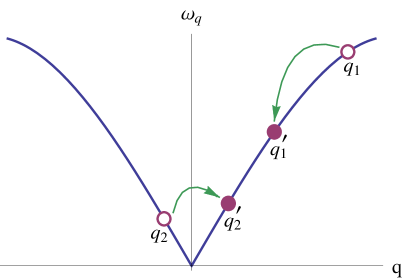
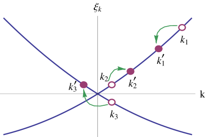
Figure 1: Leading relaxation processes for bosonic (upper panel) and fermionic (lower panel) excitations.

In the next sections we will use the Hamiltonian (LABEL:sec2:HamiltonianBosonFinal) to study the the life times of bosons and fermions in 1D interacting system. The leading processes contributing to the relaxation of bosonic and fermionic distribution functions are illustrated in Fig. 1. For bosons, this is the two-into-two scattering involving a change of the branch for one of the bosons. For fermions, these are three-fermion collisions involving in the initial state two particle from one (say, right) branch and one particle from the other (say, left) branch (see Fig. 1). We notice that both these processes arise already in the first order of perturbation theory in $\Gamma^{B,RRRL}_{\bf q}$ [This is obvious for the case of the bosonic scattering; for fermions this will become clear in Sec.IV where we discuss the fermionic form of the Hamiltonian (LABEL:sec2:HamiltonianBosonFinal)]. The momentum $q_{4}$ in $\Gamma^{B,RRRL}_{\bf q}$ has the meaning of the momentum transfer between the left and right chiral sectors in the collision process. The momentum and energy conservation dictates then the estimates $q_{4}\sim l^{2}p^{3}$ for bosonic and $q_{4}\sim p^{2}/m$ for fermionic collisions, where $p$ is the typical momentum of the right particles involved. This observation allows one to simplify dramatically the expression for the coupling $\tilde{\tilde{\Gamma}}^{B,RRRL}_{\bf q}$ by dropping all the terms which do not contain $q_{4}$ in the denominator. In this approximation we get

$$\Gamma^{B,RRRL}_{\bf q}=\frac{4\pi^{3}\alpha}{3{m^{*}}^{2}u_{0}}\left[1-\frac{3\alpha}{2}+\frac{15}{4}l^{2}\frac{q_{1}q_{2}q_{3}}{q_{4}}\right].$$ (35)

The Hamiltonian (LABEL:sec2:HamiltonianBosonFinal) with the coupling $\Gamma^{B,RRRL}_{\bf q}$ given by (35) and its fermionic version derived in Section IV constitute our starting point for the analysis of the life time of bosonic and fermionic excitations in the generic Luttinger liquid model.

III Lifetime of bosonic excitations

In this section we exploit the Hamiltonian (LABEL:sec2:HamiltonianBosonFinal) to study the decay of bosonic excitations in a dispersive Luttinger liquid.

The Fourier components of the densities $R(x)$ and $L(x)$ can be identified with bosonic creation and annihilation operators via

$$R_{q}=\sqrt{\frac{L|q|}{2\pi}}\left(\Theta(q)b_{q}+\Theta(-q)b^{+}_{-q}\right),$$

$$L_{q}=\sqrt{\frac{L|q|}{2\pi}}\left(\Theta(-q)b_{q}+\Theta(q)b^{+}_{-q}\right).$$ (36)

Let us consider a boson at momentum $Q\gtrsim T/u_{0}$ injected into the otherwise equilibrium Lutiinger liquid characterized by temperature $T$. We assume for definiteness that $Q>0$, so that we are dealing with a decay of a right moving bosonic excitation. The dominant collision process limiting the lifetime of the injected boson is a scattering on a thermal left-moving boson at momentum $q<0$ which is transfered to the right branch (see Fig.1). The lifetime of the injected boson is now given by the out-scattering term of the linearized collision integral

$$\frac{1}{\tau_{Q}(T)} = \frac{1}{2}\int\frac{dqdQ^{\prime}dq^{\prime}}{(2\pi)^{3}}W_{Qq}^{Q^{\prime}q^{\prime}}N_{B}(\omega_{q})\left(N_{B}(\omega_{Q^{\prime}})+1\right)$$ (37)

$$\times \left(N_{B}(\omega_{q^{\prime}})+1\right)\Theta(-q)\Theta(Q^{\prime})\Theta(q^{\prime}).$$

Here $N_{B}(\epsilon)$ is the equilibrium bosonic distribution function.

The transition probability $W_{Qq}^{Q^{\prime}q^{\prime}}$ can be expressed via the corresponding matrix element of the $T$-matrix

$$W_{Qq}^{Q^{\prime}q^{\prime}}=(2\pi)^{2}\left|\langle 0|b_{q^{\prime}}b_{Q^{\prime}}Tb^{+}_{Q}b^{+}_{q}|0\rangle\right|^{2}\delta\left(E_{\mathrm{i}}-E_{\mathrm{f}}\right)\\ \times\delta\left(P_{\mathrm{i}}-P_{\mathrm{f}}\right).$$ (38)

Here the $\delta$-functions express the energy and momentum conservation in the collision process.

It is easy to see that the required matrix element $\langle 0|b_{q^{\prime}}b_{Q^{\prime}}Tb^{+}_{Q}b^{+}_{q}|0\rangle$ arises in the first order of the perturbation theory in the coupling $\Gamma^{B,RRRL}_{\bf q}$ and can be read off from Eqs. (35) and (36). The result get substantially simplified since, according to the conservation laws, the momentum $q$ of the left particle is given by

$$q=-\frac{3}{2}QQ^{\prime}q^{\prime}l^{2}+{\mathrm{O}}(q^{5}l^{4}).$$ (39)

In view of this relation, the momentum-dependent and momentum-independent terms in $\Gamma^{B,RRRL}_{\bf q}$, Eq. (35), give contributions of the same form to the matrix element $\langle 0|b_{q^{\prime}}b_{Q^{\prime}}Tb^{+}_{Q}b^{+}_{q}|0\rangle$ which finally reads

$$\langle 0|b_{q^{\prime}}b_{Q^{\prime}}Tb^{+}_{Q}b^{+}_{q}|0\rangle=\frac{\pi\alpha(1+\alpha)}{m^{*2}u_{0}}\sqrt{|QQ^{\prime}qq^{\prime}|}.$$ (40)

Assuming now that the energy of the relaxing boson is much larger than temperature but is not too high ($l^{2}u_{0}Q^{3}\ll T$), one can replace the thermal factor $N_{B}(\omega_{q})$ in Eq. (37) by $1/u_{0}|q|$ and the other two thermal factors by unity. Calculating the resulting integral, we find

$$\frac{1}{\tau_{Q}(T)}=\frac{\pi\alpha^{2}(1+\alpha)^{2}}{48m^{*4}u_{0}^{4}}TQ^{4}.$$ (41)

Equation (41) gives the life time of a hot boson in our system and leads to the following estimate for a typical relaxation time of thermal bosons (i.e., those with momenta $Q\sim T/u_{0}$):

$$\frac{1}{\tau_{Q\sim T/u_{0}}(T)}\propto\frac{\alpha^{2}(1+\alpha)^{2}}{m^{*4}u_{0}^{8}}T^{5}\,,$$ (42)

up to a prefactor of order unity.

Equation (42) for the relaxation time of the bosonic excitations in the dispersive Luttinger liquid constitutes the main result of this section. The $T^{5}$ scaling of the relaxation rate of bosonic excitation has been earlier obtainedapostolov13 ; Lin2013 for a strongly interacting Luttinger liquid which is characterized by Luttinger parameter $K_{0}\ll 1$ and is close to the Wigner crystal. Our derivation is valid for any $K_{0}$ and thus represent a generalization of the result of Ref. apostolov13, ; Lin2013, . We will return to the question of the range of validity of Eq. (42) in Sec. V.

IV Lifetime of fermionic excitations

IV.1 Refermionization

The Hilbert space of a 1D chiral bosonic system is isomorphic to the Hilbert space of a 1D complex chiral fermions (more precisely, to its charge-zero sector). Correspondingly, the Hamiltonian (LABEL:sec2:HamiltonianBosonFinal) can be viewed as a Hamiltonian of fermions $c_{\eta,k},c_{\eta,k}^{+}$ introduced via

$$R_{q}=\sum_{k}c^{+}_{R,k}c_{R,k+q}\,,\qquad L_{q}=\sum_{k}c^{+}_{L,k}c_{L,k+q}.$$ (43)

As was discussed in Sec. II, the fermions are expected to be the proper excitations at momenta satisfying $m^{*}u_{0}l^{2}k\ll 1$. We are now going to discuss the life time of these low-energy fermionic quasiparticles created by the operators $c_{\eta,k}$.

We need to rephrase the Hamiltonian (LABEL:sec2:HamiltonianBosonFinal) into the fermionic language. This can be done by substituting Eq. (43) into Eq. (LABEL:sec2:HamiltonianBosonFinal) and performing the normal ordering of the resulting expression with respect to fermionic modes. It is obvious from the structure of the bosonic Hamiltonian (LABEL:sec2:HamiltonianBosonFinal) that in terms of fermions

$$H = \sum_{k}\xi_{R,k}:c^{+}_{R,k}c_{R,k}:_{F}$$ (44)

$$+ \frac{1}{L}\sum_{\bf k}\Gamma^{F,RR}_{\bf k}:c^{+}_{R,k_{1}}c^{+}_{R,k_{2}}c_{R,k_{2}^{\prime}}c_{R,k_{1}^{\prime}}:_{F}$$

$$+ \frac{1}{L}\sum_{\bf k}\Gamma^{F,RL}_{\bf k}:c^{+}_{R,k_{1}}c^{+}_{L,k_{2}}c_{L,k_{2}^{\prime}}c_{R,k_{1}^{\prime}}:_{F}$$

$$+ \frac{1}{L^{2}}\sum_{\bf k}\Gamma^{F,RRR}_{\bf k}:c^{+}_{R,k_{1}}c^{+}_{R,k_{2}}c^{+}_{R,k_{3}}c_{R,k_{3}^{\prime}}c_{R,k_{2}^{\prime}}c_{R,k_{1}^{\prime}}:_{F}$$

$$+ \frac{1}{L^{2}}\sum_{\bf k}\Gamma^{F,RRL}_{\bf k}:c^{+}_{R,k_{1}}c^{+}_{R,k_{2}}c^{+}_{L,k_{3}}c_{L,k_{3}^{\prime}}c_{R,k_{2}^{\prime}}c_{R,k_{1}^{\prime}}:_{F}$$

$$+ R\longleftrightarrow L+\ldots$$

Here the dots stand for the four-fermion interaction terms (containing eight fermionic operators). These terms do not contribute to the three-fermion collision processes which we aim to discuss in this work and we omit them altogether. We denote by ${\bf k}$ in each of vertices $\Gamma^{F,\ldots}_{\bf k}$ the set of momenta of the fermionic operators involved (e.g., ${\bf k}=(k_{1},k_{2},k_{3},k_{3}^{\prime},k_{2}^{\prime},k_{1}^{\prime})$ in the vertex $\Gamma^{F,RRL}_{\bf k}$; note the order of individual momenta in ${\bf k}$).

We refer the reader to Appendix B for details of the derivation of the couplings entering the fermionic Hamiltonian (44) and state here the final results only. First, the fermionic single-particle spectrum $\xi_{\eta,k}$ receives renormalization from the density-density interaction in (LABEL:sec2:HamiltonianBosonFinal) and is given by

$$\xi_{\eta,k}=\frac{k^{2}}{2m^{*}}+\eta\int_{0}^{k}u(k)dk\approx\eta ku_{0}+\frac{k^{2}}{2m^{*}}-\frac{\eta l^{2}u_{0}k^{3}}{3}.$$ (45)

Note that the cubic correction to the fermionic spectrum is small compared to the quadratic one at $k<1/m^{*}l^{2}u_{0}$ where the fermions are expected to be proper quasiparticles of the system.

The two-particle intrabranch interaction in the fermionic Hamiltonian (44) arises from the intrabranch density-density interaction in (LABEL:sec2:HamiltonianBosonFinal),

$$\Gamma^{F,RR}_{\bf k}=\frac{\pi u_{0}l^{2}}{2}(k_{1}-k_{2})(k_{1}^{\prime}-k_{2}^{\prime}).$$ (46)

Here we have take into account the expansion of the bosonic velocity $u_{q}$ at small momenta. The vertex $\Gamma^{RR}_{\bf k}$ also receives corrections from the cubic-in-density intrabranch bosonic coupling $\Gamma^{B,RRR}_{\bf q}$. These corrections are however parametrically small, and we neglect them.

The interbranch two- and three-particle couplings, which will be most important for our analysis of the relaxation, both arise from the bosonic vertex $\Gamma^{B,RRRL}_{\bf q}$, Eqs. (LABEL:sec2:HamiltonianBosonFinal), (35). Remarkably, a singularity at small momentum transfer $k_{3}-k_{3}^{\prime}$ which might be expected in view of the last term in Eq. (35) does not show up in $\Gamma^{RL}_{\bf k}$. This vertex is mostly determined by the first, momentum-independent term in (35) and is given by

$$\Gamma^{F,RL}_{\bf k}=\Gamma^{F,LR}_{\bf k}=\frac{\pi\alpha(2-3\alpha)}{2m^{*2}u_{0}}k_{1}k_{1}^{\prime}.$$ (47)

On the contrary, the three-fermion coupling $\Gamma^{F,RRL}_{\bf k}$ emerges solely due to the last term in Eq. (35),

$$\Gamma^{F,RRL}_{\bf k} = \frac{5\alpha l^{2}\pi^{2}(k_{1}-k_{2})(k_{1}^{\prime}-k_{2}^{\prime})}{16m^{*2}u_{0}(k_{3}-k_{3}^{\prime})}$$ (48)

$$\times \left[(k_{1}-k_{2})^{2}-(k_{1}^{\prime}-k_{2}^{\prime})^{2}\right].$$

and is singular at $k_{3}-k_{3}^{\prime}=0$.

Let us finally comment on the three-particle intrabranch interaction vertex $\Gamma^{F,RRR}_{\bf k}$. It arises from the cubic intrabranch coupling in the bosonic Hamiltonian (LABEL:sec2:HamiltonianBosonFinal). By construction, $\Gamma^{F,RRR}_{\bf k}$ is antisymmetric in the three incoming ($k_{1}$, $k_{2}$, $k_{3}$) and the three outgoing momenta $k_{1}^{\prime}$, $k_{2}^{\prime}$ and $k_{3}^{\prime}$. Since the bosonic vertex $\Gamma^{B,RRR}_{\bf q}$ is analytic at small momenta, $\Gamma^{F,RRR}_{\bf k}$ should be of the form

$$\Gamma^{F,RRR}_{\bf k}\propto\frac{l^{6}}{m^{*}}\prod_{i>j}(k_{i}-k_{j})(k_{i}^{\prime}-k_{j}^{\prime}).$$ (49)

We thus see that $\Gamma^{F,RRR}_{\bf k}$ is strongly suppressed by a high power of the momenta. In fact, it is exactly zero withing our approximation for the bosonic coupling $\Gamma^{B,RRR}_{\bf q}$, Eq. (17). One needs to retain the sixth-order terms in the expansion of $\Gamma^{B,RRL}_{\bf q}$ over momentum to generate non-zero $\Gamma^{F,RRR}_{\bf k}$. From now on we will largely ignore $\Gamma^{F,RRR}_{\bf k}$ apart from a short discussion of the intrabranch fermionic relaxation processes at the end of the Sec. IV.2.

With the fermionic Hamiltonian (44) and the couplings (46), (47), (48) at hand, we are now in a position to study the life time of the fermionic excitations in our problem. Below we employ the perturbation theory in the fermionic interaction terms $\Gamma^{F,\eta\eta^{\prime}}_{\bf k}$ and $\Gamma^{F,RRL}_{\bf k}$ to evaluate the corresponding scattering rate.

IV.2 Fermionic scattering rate

Here we calculate the life time of fermionic excitations in a dispersive Luttinger liquid. The relaxation of the fermionic distribution function is governed by the three-particle collisions. At zero temperature the intrabranch collision processes (with all three particles in the initial and final states residing on the right branch) are ruled out by the energy and momentum conservation. At finite temperature, the situation we consider in this work, both intrabranch collisions and the scattering events involving the creation of a particle-hole pair in the left branch (see Fig. 1) contribute to the relaxation of a right-moving fermion injected into the system. However, the intrabranch collision rate $1/\tau^{RRR}(T)$ turns out to be proportional to a very high power of temperature ($T^{14}$) and is small compared to the interbranch collision rate $1/\tau^{RRL}(T)$ in the whole “fermionic” part of the parameter space. We will discuss this point in more detail at the end of this section and concentrate now on the contribution of interbranch collisions to the decay of fermionic quasiparticles.

The decay rate $1/\tau_{k_{1}}^{RRL}(T)$ of a fermion with momentum $k_{1}\gtrsim T/u_{0}$ is given by the out-scattering term of the linearized three-particle collision integral,

$$1/\tau^{RRL}_{k_{1}}(T) = \frac{1}{2}\int\left(d{\bf k}\right)W_{k_{1},k_{2},k_{3}}^{k_{1}^{\prime},k_{2}^{\prime},k_{3}^{\prime}}N_{F}(\xi_{R,k_{2}})N_{F}(\xi_{L,k_{3}})$$ (50)

$$\times \left(1-N_{F}(\xi_{R,k_{1}^{\prime}})\right)\left(1-N_{F}(\xi_{R,k_{2}^{\prime}})\right)$$

$$\times \left(1-N_{F}(\xi_{L,k_{3}^{\prime}})\right).$$

Here $(d{\bf k})=dk_{2}dk_{3}dk_{1}^{\prime}dk_{2}^{\prime}dk_{3}^{\prime}/(2\pi)^{5}$ and $N_{F}(\epsilon)$ stands for the Fermi-Dirac distribution at temperature $T$. The transition probability $W_{k_{1},k_{2},k_{3}}^{k_{1}^{\prime},k_{2}^{\prime},k_{3}^{\prime}}$ entering Eq. (50) is given by the modulus squared of the appropriate entry of the $T$-matrix,

$$W_{k_{1},k_{2},k_{3}}^{k_{1}^{\prime},k_{2}^{\prime},k_{3}^{\prime}} = (2\pi)^{2}\left|\langle 1,2,3|T|1^{\prime},2^{\prime},3^{\prime}\rangle\right|^{2}$$ (51)

$$\times \delta\left(E_{\mathrm{i}}-E_{\mathrm{f}}\right)\delta\left(P_{\mathrm{i}}-P_{\mathrm{f}}\right)\,.$$

Here the $\delta$-functions express the conservation of energy and momentum in the collision process and

$$|1,2,3\rangle=c^{+}_{R,k_{1}}c^{+}_{R,k_{2}}c^{+}_{L,k_{3}}|0\rangle.$$ (52)

Examination of the fermionic Hamiltonian (44) shows that to the leading order in $1/m$ there are two contributions to the matrix element $\langle 1,2,3|T|1^{\prime},2^{\prime},3^{\prime}\rangle$. The first one stems from the three-fermion coupling $\Gamma^{F,RRL}_{k}$ in the first order of perturbation theory and is given by

$$\langle 1,2,3|T|1^{\prime},2^{\prime},3^{\prime}\rangle_{1}=4\Gamma^{F,RRL}_{k_{1}^{\prime},k_{2}^{\prime},k_{3}^{\prime},k_{3},k_{1},k_{2}},$$ (53)

where the vertex $\Gamma^{F,RRL}_{k}$ is given by (48). The second contribution arises in the second order of the perturbation theory in the two-fermion couplings $\Gamma^{RR}_{\bf k}$ and $\Gamma^{RL}_{\bf k}$,

$$\langle 1,2,3|T|1^{\prime},2^{\prime},3^{\prime}\rangle_{2}\\ =\frac{8\Gamma^{F,RR}_{k_{1}^{\prime},k_{2}^{\prime},k_{2},q}\left(\Gamma^{F,RL}_{q,k_{3}^{\prime},k_{3},k_{1}}+\Gamma^{F,LR}_{q,k_{3}^{\prime},k_{3},k_{1}}\right)}{\xi_{L,k_{3}}-\xi_{L,k_{3}^{\prime}}+\xi_{R,k_{1}}-\xi_{R,q}}\\ +\frac{8\Gamma^{F,RR}_{k_{1}^{\prime},q,k_{2},k_{1}}\left(\Gamma^{F,RL}_{k_{2}^{\prime},k_{3}^{\prime},k_{3},q}+\Gamma^{F,LR}_{k_{2}^{\prime},k_{3}^{\prime},k_{3},q}\right)}{\xi_{L,k_{3}^{\prime}}-\xi_{L,k_{3}}+\xi_{R,k_{2}^{\prime}}-\xi_{R,q}}.$$ (54)

In Eq. (54) we implicitly assume the anti-symmetrization of the right-hand side with respect to permutations of $k_{1}$ and $k_{2}$ as well as $k_{1}^{\prime}$ and $k_{2}^{\prime}$. The momentum $q$ of the intermediate virtual state in Eq. (54) is fixed by the momentum conservation in the vertices $\Gamma^{F,RL}_{\bf k}$ implying that $q=k_{1}+k_{3}-k_{3}^{\prime}$ for the first term and $q=k_{2}^{\prime}+k_{3}^{\prime}-k_{3}$ for the second one.

Let us now consider the energy denominators in (54) in more detail. Using the explicit form (45) of the single-particle dispersion relations, one finds for the first energy denominator

$$\xi_{L,k_{3}}-\xi_{L,k_{3}^{\prime}}+\xi_{R,k_{1}}-\xi_{R,q}\\ =-2u_{0}(k_{3}-k_{3}^{\prime})[1+O(k/p_{F})+O(k^{2}l^{2})],$$ (55)

with $k$ being the characteristic value of the momenta. The second denominator in (54) has exactly the same structure. Working to the leading order in $k/p_{F}$ , $k^{2}l^{2}$ and using explicit expressions for the vertices $\Gamma^{F,RR}_{\bf k}$, $\Gamma^{F,RL}_{\bf k}$ derived earlier, we get (after the proper anti-symmetrization over momenta)

$$\langle 1,2,3|T|1^{\prime},2^{\prime},3^{\prime}\rangle_{2}\\ =\frac{\pi^{2}\alpha(2-3\alpha)l^{2}(k_{1}-k_{2})(k_{1}^{\prime}-k_{2}^{\prime})}{2m^{*2}u_{0}(k_{3}-k_{3}^{\prime})}\\ \times\left(k_{1}^{2}+k_{2}^{2}+4k_{1}k_{2}-k_{1}^{\prime 2}-k_{2}^{\prime 2}-4k_{1}^{\prime}k_{2}^{\prime}\right).$$ (56)

Let us assume from now on that the the temperature of the system is low, $m^{*}l^{2}T\ll 1$, i.e, we are in the situation when the fermions are expected to be the proper quasiparticles for the description of the system. Under this condition we can neglect the cubic term in the fermionic dispersion relation (45). The matrix elements (53) and (56) can be further simplified if one takes into account the energy conservation in the collision process. First, we note that the energy and momentum conservation requires that at zero momentum transfer $k_{3}-k_{3}^{\prime}=0$ the right-moving particles can only preserve or exchange their momenta. Thus, the singularity in the matrix elements (53) and (56) is canceled if we consider them on the mass shell. Second, on the mass shell the momentum transfer can be estimated as $k_{3}-k_{3}^{\prime}\sim k^{2}/m^{*}u_{0}$, where $k$ is the characteristic momentum of the colliding particles. Consequently, we can estimate the matrix elements (53) and (56) on the mass shell as

$$\langle 1,2,3|T|1^{\prime},2^{\prime},3^{\prime}\rangle_{1(2)}\propto\frac{l^{2}(k_{1}-k_{2})(k_{1}^{\prime}-k_{2}^{\prime})}{m^{*}}.$$ (57)

The accurate calculation presented in Appendix C confirms this estimate and yieldsRemark_T

$$\langle 1,2,3|T|1^{\prime},2^{\prime},3^{\prime}\rangle=\frac{6\pi^{2}\alpha(1+\alpha)l^{2}(k_{1}-k_{2})(k_{1}^{\prime}-k_{2}^{\prime})}{m^{*}}.$$ (58)

Assuming now that the energy of the relaxing particle $u_{0}k_{1}$ is not too high ($u_{0}k_{1}\ll\sqrt{Tu_{0}^{2}m^{*}}$) one can linearize the fermionic spectra in the energy conserving $\delta$-function in Eq.(51). The integration over $k_{3}$ and $k_{3}^{\prime}$ is Eq.(50) is then straightforward and leads to

$$1/\tau^{RRL}_{k_{1}}(T)=\frac{T}{8\pi u_{0}^{2}}\int\frac{dk_{2}dk_{1}^{\prime}dk_{2}^{\prime}}{(2\pi)^{3}}T_{k_{1},k_{2}}^{k_{1}^{\prime},k_{2}^{\prime}}N_{F}(\xi_{R,k_{2}^{\prime}})\\ \times\left(1-N_{F}(\xi_{R,k_{1}^{\prime}})\right)\left(1-N_{F}(\xi_{R,k_{2}^{\prime}})\right)2\pi\delta(k_{1}+k_{2}-k_{1}^{\prime}-k_{2}^{\prime})$$ (59)

At $k_{1}\gg T/u_{0}$ we can approximate the Fermi distributions entering (59) by the zero-temperature ones, which leads to the following result for the relaxation rate of a hot fermion in our system:

$$1/\tau^{RRL}_{k_{1}}(T)=\frac{11\pi\alpha^{2}(1+\alpha)^{2}l^{4}Tk_{1}^{6}}{80m^{*}u_{0}^{2}}.$$ (60)

The corresponding estimate for the lifetime of the thermal quasiparticles with $k_{1}\sim T/u_{0}$ constitutes the central result of this section

$$1/\tau^{RRL}_{k_{1}\sim T/u_{0}}(T)\propto\frac{\alpha^{2}(1+\alpha)^{2}l^{4}T^{7}}{m^{*2}u_{0}^{8}}.$$ (61)

Equation (61) establishes the relaxation rate of the fermionic quasiparticles in a general dispersive Luttinger liquid. Its scaling with temperature coincides with the one obtained previously for weakly interacting fermions within a perturbation theory imambekov11 and for fermionic quasiparticles of a Luttinger liquid with a short-range interaction MatveevFurusaki2013 . The $T^{7}$ scaling in Eq. (61) can be traced back to a product of $T^{4}$ factor arising due to the quadratic scaling of the matrix element (58) with the momentum and a $T^{3}$ factor steming from the phase volume.

We return now to the scattering rate $1/\tau^{RRR}_{k_{1}}(T)$ induced by intrabranch three-particle collisions. The corresponding amplitude $\langle 123|T|1^{\prime}2^{\prime}3^{\prime}\rangle$ (with all the particle belonging now to the right branch) arises in the first order of the perturbation theory over the vertex $\Gamma^{F,RRR}_{\bf k}$ as well as in the second order in the intrabranch two-particle interaction $\Gamma^{F,RR}_{\bf k}$. The matrix element induced by $\Gamma^{F,RRR}_{\bf k}$ is given by [see Eq. (49)]

$$\langle 123|T|1^{\prime}2^{\prime}3^{\prime}\rangle_{1}\propto\frac{l^{6}}{m^{*}}\prod_{i>j}(k_{i}-k_{j})(k_{i}^{\prime}-k_{j}^{\prime}).$$ (62)

A careful examination of the second order of the perturbation theory in $\Gamma^{F,RR}_{\bf k}$ shows that, despite the presence of energy denominators, the corresponding matrix element $\langle 123|T|1^{\prime}2^{\prime}3^{\prime}\rangle_{2}$ is non-singular at the mass shell and has the same momentum dependence (dictated by indistinguishability of the particles) as Eq. (62),

$$\langle 123|T|1^{\prime}2^{\prime}3^{\prime}\rangle_{2}\propto m^{*}u_{0}^{2}l^{8}\prod_{i>j}(k_{i}-k_{j})(k_{i}^{\prime}-k_{j}^{\prime}).$$ (63)

To obtain Eq. (63) one has to go beyond the approximation (4) for the momentum-dependent bosonic velocity and the corresponding approximation (46) for the intrabranch two-particle interaction $\Gamma^{RR}_{\bf k}$. Specifically, one has to retain the $O(k^{4})$ terms for both vertices $\Gamma^{RR}_{k}$ involved. This is the reason for the appearance of the factor $l^{8}$ in (63). The factor of mass $m^{*}$ in Eq. (63) comes from the energy denominator of the second-order perturbation theory and reflects its degenerate nature for dispersionless fermions.

Comparing Eqs. (62) and (63), we observe that the second contribution dominates due to an additional factor $(m^{*}u_{0}l)^{2}\gtrsim 1$, so that the matrix element for the intrabranch triple collisions is given by Eq. (63). The evaluation of the intrabranch transition rate is now a matter of power counting resulting in

$$1/\tau^{RRR}_{k_{1}\sim T/u_{0}}(T)\propto\frac{m^{*3}l^{16}T^{14}}{u_{0}^{10}}.$$ (64)

The second power of mass in Eq. (64) comes from the matrix element (63) and an additional factor $m^{*}$ arises from the $\delta$-function expressing the energy conservation due to the fact that energy and momentum conservation coincide for particles with the linear spectrum. Comparing (64) to (61), we see that the interbranch collision processes dominate in the entire range of temperatures $m^{*}l^{2}T/u_{0}\ll 1$ where the above fermionic analysis is justified.

V Fermi-Bose weak-strong-coupling duality

In the previous sections we have presented a detailed analysis of relaxation times of bosonic and fermionic excitations in a dispersive Luttinger liquid. For this purpose, we have carried out a perturbative treatment of the Hamiltonian (LABEL:sec2:HamiltonianBosonFinal) and of its fermionized version (44), respectively. Comparing now the two calculations above, we observe that the fermionic and bosonic relaxations are closely related: they both originate from the same interaction term $\Gamma^{RRRL}_{\bf q}$ in the Hamiltonian (LABEL:sec2:HamiltonianBosonFinal) and are both dominated by the processes with small momentum transfer between the right and left chiral branches. An important difference between the bosonic and fermionic scattering processes is the scaling of this momentum transfer with the typical momentum of the right particles, which is cubic for bosons and quadratic for fermions.

Comparison of the bosonic and fermionic relaxation times, Eqs. (42) and (61), reveals the dimensionless parameter $\lambda=m^{*}l^{2}T$ anticipated in Sec. II. In agreement with the qualitative discussion in Sec. II, at low temperatures, $\lambda\ll 1$, the result (61) for the decay rate of fermionic excitations in a dispersive Luttinger liquid is much smaller than Eq. (42) resulting from a bosonic perturbative treatment of the Hamiltionian (LABEL:sec2:HamiltonianBosonFinal). Thus, fermions are proper excitations in this regime. The situation is reverse at high temperatures where $\lambda\gg 1$.

To support this subdivision of the parameter space in “fermionic” and “bosonic” domains, let us analyze the perturbation theories used in the previous sections to evaluate the bosonic and fermionic lifetimes. We consider first the fermionic formalism. As follows from Eq. (45), a finite interaction radius $l_{\rm int}$ induces a cubic correction to the spectrum of the fermionic quasiparticles. This correction is small in comparison to the original curvature $1/m^{*}$ at momenta $k\ll 1/m^{*}u_{0}l^{2}$, yielding the condition $\lambda\ll 1$ for the fermionic perturbation theory. Furthermore, an estimate for the scaling of higher-order diagrams (with 4, 5, …fermions involved) confirms that the perturbation theory is controlled by the parameter $\lambda\ll 1$. Conversely, a finite fermionic mass broadens the support of the dynamical structure factor in the frequency-momentum plane $(\omega,q)$ by an amount of the order of $\delta\omega\sim q^{2}/m^{*}$. This broadening exceeds the nonlinear bending of the bosonic single-particle spectrum $u_{0}l^{2}q^{3}$ at momenta $q\lesssim 1/m^{*}u_{0}l^{2}$ and makes the perturbative treatment of the bosonic Hamiltonian inadequate for $\lambda\lesssim 1$. In other words, a small parameter controlling the bosonic perturbation theory is $\lambda^{-1}\ll 1$. To summarize, the fermionic and bosonic descriptions of a dispersive Luttinger liquid are characterized by the coupling constants $\lambda$ and $\lambda^{-1}$, respectively, thus showing a remarkable weak-strong-coupling duality.

The “phase diagram” of a dispersive Luttinger liquid exhibiting a crossover between the bosonic and fermionic regimes is shown in Fig. 2 in the coordinates $(Tl/u_{0},\ T/m^{*}u_{0}^{2})$.

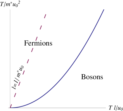
Figure 2: “Phase diagram” of a dispersive Luttinger liquid in the parameter plane $(x=Tl/u_{0},\ y=T/m^{*}u_{0}^{2})$. Relaxation rates in the bosonic and fermionic parts of the phase diagram are given by Eqs. (42) and (61), respectively. The solid line $y=x^{2}$ indicates a crossover between the fermionic and bosonic regimes. The dashed line corresponds to the minimal physically sensible interaction length $l\sim 1/m^{*}u_{0}$.

VI Summary and outlook

To summarize, we have explored the life time of excitations in a dispersive Luttinger liquid in the whole range of parameters. We employed bosonization approach supplemented by a sequence of unitary transformations to a quasiparticle representations which allowed us to eliminate many of interaction-induced contributions from the Hamiltonian. The resulting bosonic Hamiltonian is given by Eq. (LABEL:sec2:HamiltonianBosonFinal) and its refermionized version by Eq. (44).

We have performed both bosonic and fermionic analysis of the relaxation rate in this formalism. The central results of this work, Eqs. (42) and (61), reveal the Bose-Fermi weak-strong coupling duality controlled by the parameter $\lambda=m^{*}l^{2}T$ and allow us to establish the “Bose-Fermi phase diagram” of a generic dispersive Luttinger liquid presented in Fig. 2.

Remarkably, the parameter $\lambda$ controlling the Bose-Fermi crossover in the relaxation mechanisms studied in this work is closely related to the parameter $\lambda_{\rho}=u_{0}m^{*}l^{2}\Delta\rho$ which was shown recentlyPGM2013 ; protopopov13 to govern the character of the collisionless evolution of a density perturbation with an amplitude $\Delta\rho$ in a dispersive Luttinger liquid. Specifically, it was found in Ref. PGM2013, that for $\lambda_{\rho}\ll 1$ (“fermionic” regime) the corresponding collisionless kinetic equation predicts a formation of the population inversion in the distribution function of fermions while for $\lambda_{\rho}\gg 1$ (“bosonic” regime) no such phenomenon occurs and the density evolution follows closely the predictions of a hydrodynamic theory. Comparing the expressions for $\lambda$ and $\lambda_{\rho}$, we observe that they are identical, up to a replacement of the characteristic energy scale $T$ by $u_{0}\Delta\rho$. In this context, our present findings open up the possibility to incorporate the relaxation processes into the description of the pulse propagation in dispersive Luttinger liquids. In the “fermionic” regime the fermionic collisions studied in this work can be directly included into kinetic equation of Ref. PGM2013, . On the other hand, a proper account for the relaxation processes in the “bosonic” regime of the pulse propagation requires a formulation of a bosonic version of the kinetic equation, which remains a prospect for future research.

Another direction for future work is the investigation of a broader class of interaction potentials within our formalism. In particular, it would be interesting to study the Fermi-Bose duality in relaxation of excitations in the case of power-law ($1/r^{\alpha}$) interactions. Especially important, in view of applications to charged fermions, is the case of Coulomb ($1/r$) interaction screened (e.g., due to a remote gate) at a large distance $d\gg p_{F}^{-1}$. We also envision an extension of our approach to the situation when the initial interacting particles are bosons, which is relevant in the context of the physics of cold atoms in one-dimensional traps.

Appendix A Unitary transformation $U_{3}$ and bosonic vortexes

In this Appendix we derive explicit expressions for the bosonic vertices $\Gamma^{B,RRRR}_{\bf q}$, $\Gamma^{B,RRRL}_{\bf q}$ and $\Gamma^{B,RRLL}_{\bf q}$. Our starting point is the Hamiltonian after the unitary rotation $U_{2}$, see Eq. (14). In terms of the new density operators $\tilde{\rho}_{\eta}$ the Hamiltonian reads

$$H = (\pi/L)\sum_{q}u_{q}:\left(\tilde{\rho}_{R,q}\tilde{\rho}_{R,-q}+\tilde{\rho}_{L,q}\tilde{\rho}_{L,-q}\right):_{B}$$ (65)

$$+ \frac{1}{L^{2}}\sum_{{\bf q}}\left[\Gamma^{B,RRR}_{\bf q}:(\tilde{\rho}_{R,q_{1}}\tilde{\rho}_{R,q_{2}}\tilde{\rho}_{R,q_{3}}+R\rightarrow L):_{B}\right.$$

$$+ \left.\Gamma^{B,RRL}_{\bf q}:(\tilde{\rho}_{R,q_{1}}\tilde{\rho}_{R,q_{2}}\tilde{\rho}_{L,q_{3}}+R\leftrightarrow L):_{B}\right]$$

$$\equiv H^{(2)}+H^{(3)}_{D}+H^{(3)}_{O}\,.$$

Here we have splitted the Hamiltonian into the quadratic part $H^{(2)}$, the diagonal-in-chiralities cubic part $H^{(3)}_{D}$ and the chirality-mixing cubic part $H^{(3)}_{O}$.

Expressing now the densities $\tilde{\rho}_{R(L)}$ via Eq. (LABEL:sec2:DensityExpansion), we find

$$H = H^{(2)}+H^{(3)}_{D}+H^{(3)}_{O}-\left[\Omega_{3},H^{(2)}\right]$$ (66)

$$- \left[\Omega_{3},H^{(3)}_{D}+H^{(3)}_{O}\right]+\frac{1}{2}\left[\Omega_{3},\left[\Omega_{3},H^{(2)}\right]\right]$$

$$+ {\mathrm{O}}(\rho^{5})\,.$$

The operators $H^{(2)}$, $H^{(3)}_{D(O)}$ in the right hand side of Eq.(66) are obtained from that of Eq.(65) by a simple replacement $\tilde{\rho}_{R(L)}\rightarrow R(L)$.

The decoupling of the chiral sectors in the third order requires that

$$\left[\Omega_{3},H^{(2)}\right]=H^{(3)}_{O}\,,$$ (67)

which is equivalent to Eq. (26). Using Eq. (67), one can bring Eq. (66) to a simpler form

$$H=H^{(2)}+H^{(3)}_{D}-\left[\Omega_{3},H^{(3)}_{D}+\frac{1}{2}H^{(3)}_{O}\right]+{\mathrm{O}}(\rho^{5})\,.$$ (68)

Computing the commutator, we obtain the following result for the fourth-order correction to the Hamiltonian:

$$H^{(4)} = \frac{1}{2\pi L^{3}}\sum_{{\bf q},p}\left[-6p\Gamma^{B,RRR}_{-p,q_{1},q_{2}}f_{p,q_{3},q_{4}}+p\Gamma^{B,RRL}_{-p,q_{4},q_{3}}f_{q_{1},q_{2},p}-p\Gamma^{B,RRL}_{q_{1},q_{2},-p}f_{p,q_{4},q_{3}}\right]\left[\left(R_{q_{1}}R_{q_{2}}R_{q_{3}}\right)_{s}L_{q_{4}}+R\leftrightarrow L\right]$$ (69)

$$+ \frac{1}{2\pi L^{3}}\sum_{{\bf q},p}\left[3p\Gamma^{B,RRR}_{-p,q_{1},q_{2}}f_{q_{3},q_{4},p}+3p\Gamma^{B,RRR}_{-p,q_{3},q_{4}}f_{q_{1},q_{2},p}-2p\Gamma^{B,RRL}_{-p,q_{1},q_{3}}f_{p,q_{2},q_{4}}-2p\Gamma^{B,RRL}_{-p,q_{3},q_{1}}f_{p,q_{4},q_{2}}\right]\left(R_{q_{1}}R_{q_{2}}\right)_{s}\left(L_{q_{3}}L_{q_{4}}\right)_{s}$$

$$+ \frac{1}{4\pi L^{3}}\sum_{{\bf q},p}p\Gamma^{B,RRL}_{q_{1},q_{2},-p}f_{q_{3},q_{4},p}\left[\left(R_{q_{1}}R_{q_{2}}R_{q_{3}}R_{q_{4}}\right)_{s}+R\rightarrow L\right].$$

Here the subscript $s$ in the expressions of the type $\left(\ldots\right)_{s}$ stands for a symmetrization of the expression inside brackets with respect to the momenta $q_{i}$.

Comparing Eq. (69) to Eq. (28), one can read off explicit expressions for fourth-order bosonic vertices [$\Gamma^{B,RRRR}_{\bf q}$ etc.] in terms of $\Gamma^{B,RRR}_{\bf q}$ and $\Gamma^{B,RRL}_{\bf q}$. Exploiting the expansion of third-order vertices at small momenta, we get

$$\Gamma^{B,\mu\nu\rho\kappa}_{\bf q}\approx\tilde{\Gamma}^{B,\mu\nu\rho\kappa}_{\bf q}+l^{2}\tilde{\tilde{\Gamma}}^{B,\mu\nu\rho\kappa}_{\bf q}\,,\qquad q^{2}l^{2}\ll 1\,,$$ (70)

with

$$\tilde{\Gamma}^{B,RRRR}_{\bf q} = -\frac{\pi^{3}\alpha^{2}}{2u_{0}{m^{*}}^{2}},\qquad$$ (71)

$$\tilde{\Gamma}^{B,RRRL}_{\bf q} = \frac{4\pi^{3}\alpha}{3{m^{*}}^{2}u_{0}}\left[1-\frac{3\alpha}{2}-\frac{\alpha}{4}\left(\frac{q_{4}}{q_{1}}+\frac{q_{4}}{q_{2}}+\frac{q_{4}}{q_{3}}\right)\right],$$

and

$$\tilde{\tilde{\Gamma}}^{B,RRRL}_{\bf q} = \frac{5\pi^{3}\alpha}{{m^{*}}^{2}u_{0}}$$ (73)

$$\times \left[\frac{q_{1}q_{2}q_{3}}{q_{4}}+\frac{(6-13\alpha)}{20}\left(q_{1}^{2}+q_{2}^{2}+q_{3}^{2}\right)\right.$$

$$- \left.\frac{\alpha}{30}q_{4}\left(\frac{q_{1}^{2}+q_{2}^{2}}{q_{3}}+\frac{q_{1}^{2}+q_{3}^{2}}{q_{2}}+\frac{q_{2}^{2}+q_{3}^{2}}{q_{1}}\right)\right.$$

$$+ \frac{26\alpha-53\alpha^{2}-8}{60\alpha}q_{4}^{2}$$

$$+ \left.\frac{1-5\alpha}{30}q_{4}^{3}\left(\frac{1}{q_{1}}+\frac{1}{q_{2}}+\frac{1}{q_{3}}\right)\right].$$

For completeness we present also the amplitude $\Gamma^{B,RRLL}_{\bf q}$ although we do not need it in the main text:

$$\tilde{\Gamma}^{B,RRLL}_{\bf q} = \frac{\pi^{3}\alpha}{{m^{*}}^{2}u_{0}}\left[1+\frac{\alpha\left(q_{1}-q_{2}\right)^{2}}{2q_{1}q_{2}}\right]+R\leftrightarrow L,$$

$$\tilde{\tilde{\Gamma}}^{B,RRLL}_{\bf q} = \frac{\pi^{3}\alpha}{{8m^{*}}^{2}u_{0}L^{3}}\left[(16-47\alpha)\left(q_{1}^{2}+q_{2}^{2}\right)\right.$$ (75)

$$- \frac{\left(4-3\alpha^{2}\right)}{\alpha}(q_{1}+q_{2})^{2}$$

$$+ 17\alpha\left(q_{1}^{2}+q_{2}^{2}\right)\left(\frac{q_{3}}{q_{4}}+\frac{q_{4}}{q_{3}}\right)$$

$$- \left.(5\alpha+2)\left(\frac{q_{1}^{3}}{q_{2}}+\frac{q_{2}^{3}}{q_{1}}\right)\right]$$

$$+ R\leftrightarrow L\,.$$

Appendix B Fermionic form of the Hamiltonian

In this Appendix we present a detailed derivation of the fermionized form of the bosonic Hamiltonian (LABEL:sec2:HamiltonianBosonFinal). It is obvious from the structure of the Hamiltonian (LABEL:sec2:HamiltonianBosonFinal) that in terms of fermions

$$H = \sum_{k}\xi_{R,k}:c^{+}_{R,k}c_{R,k}:_{F}$$ (76)

$$+ \frac{1}{L}\sum_{\bf k}\Gamma^{F,RR}_{\bf k}:c^{+}_{R,k_{1}}c^{+}_{R,k_{2}}c_{R,k_{2}^{\prime}}c_{R,k_{1}^{\prime}}:_{F}$$

$$+ \frac{1}{L}\sum_{\bf k}\Gamma^{F,RL}_{\bf k}:c^{+}_{R,k_{1}}c^{+}_{L,k_{2}}c_{L,k_{2}^{\prime}}c_{R,k_{1}^{\prime}}:_{F}$$

$$+ \frac{1}{L^{2}}\sum_{\bf k}\Gamma^{F,RRR}_{\bf k}:c^{+}_{R,k_{1}}c^{+}_{R,k_{2}}c^{+}_{R,k_{3}}c_{R,k_{3}^{\prime}}c_{R,k_{2}^{\prime}}c_{R,k_{1}^{\prime}}:_{F}$$

$$+ \frac{1}{L^{2}}\sum_{\bf k}\Gamma^{F,RRL}_{\bf k}:c^{+}_{R,k_{1}}c^{+}_{R,k_{2}}c^{+}_{L,k_{3}}c_{L,k_{3}^{\prime}}c_{R,k_{2}^{\prime}}c_{R,k_{1}^{\prime}}:_{F}$$

$$+ R\longleftrightarrow L+\ldots$$

Here $\ldots$ stand for the four-fermion interactions (i.e, those involving eight fermionic operators). In each of vertices $\Gamma^{F,\ldots}_{\bf k}$, we denote by ${\bf k}$ the vector of momenta of the fermionic operators involved. (As an example, ${\bf k}=(k_{1},k_{2},k_{3},k_{3}^{\prime},k_{2}^{\prime},k_{1}^{\prime})$ in the vertex $\Gamma^{F,RRL}_{\bf k}$.) To derive explicit expressions for the fermionic vertices $\Gamma^{F,\ldots}_{\bf k}$, one substitutes the expansions (43) into (LABEL:sec2:HamiltonianBosonFinal) and performs the normal ordering of resulting expressions with respect to fermionic operators. In the rest of this Appendix we analyze these vertices one by one.

B.1 Single-particle spectrum $\xi_{\eta,k}$

The quadratic part of the fermionic Hamiltonian stems from the quadratic and the cubic terms in the bosonic Hamiltonian (LABEL:sec2:HamiltonianBosonFinal). For the sake of clarity, we concentrate here on the single-particle spectrum of the right fermions. To compute $\xi_{R,k}$, we consider

$$H^{RR+RRR} = (\pi/L)\sum_{q}u_{q}:R_{q}R_{-q}:_{B}$$ (77)

$$+ \frac{1}{L^{2}}\sum_{{\bf q}}\Gamma^{B,RRR}_{\bf q}:R_{q_{1}}R_{q_{2}}R_{q_{3}}:_{B}.$$

with the densities re-expressed in term of the fermionic operators and perform the normal ordering with respect to fermions, retaining only the contributions quadratic in fermions. Neglecting first the momentum dependence of $\Gamma^{B,RRR}_{\bf q}$, we get

$$\xi_{R,k}=\frac{k^{2}}{2m^{*}}+\int_{0}^{q}du_{q}\approx u_{0}k+\frac{k^{2}}{2m^{*}}-\frac{l^{2}k^{3}}{3}.$$ (78)

A quick estimate shows that the contribution of the momentum-dependent terms in the expansion of $\Gamma^{B,RRR}_{\bf q}$ is of the order $l^{2}k^{4}/m^{*}$ and is always small.

B.2 Intrabranch two-particle vertex $\Gamma^{F,RR}_{\bf k}$

Just as the single-particle spectrum, the coupling $\Gamma^{F,RR}_{\bf k}$ arises from the terms (77) of the bosonic Hamiltonian. The contribution of the quadratic part of the bosonic Hamiltonian is easily found to be

$$\Gamma^{F,RR}_{\bf k}=\frac{\pi u_{0}l^{2}}{2}(k_{1}-k_{2})(k_{1}^{\prime}-k_{2}^{\prime}).$$ (79)

As for the cubic coupling $\Gamma^{B,RRR}_{\bf q}$, its zero momentum part does not contribute to $\Gamma^{F,RR}_{\bf k}$, while the contribution of its $O(q^{2})$ terms is of the order $k^{3}l^{2}/m^{*}$ and can be neglected.

B.3 Interbranch two-particle vertices $\Gamma^{F,RL}_{\bf k}$ and $\Gamma^{F,LR}_{\bf k}$

We turn now to a derivation of the fermionic vertex $\Gamma^{F,RL}_{\bf k}$ and $\Gamma^{F,LR}_{\bf k}$ entering the two-particle interaction between left and right sectors of the theory,

$$\delta H = \frac{1}{L}\sum_{\bf k}\Gamma^{F,RL}_{\bf k}:c^{+}_{R,k_{1}}c^{+}_{L,k_{2}}c_{L,k_{2}^{\prime}}c_{R,k_{1}^{\prime}}:_{F}$$ (80)

$$+ \frac{1}{L}\sum_{\bf k}\Gamma^{F,LR}_{\bf k}:c^{+}_{L,k_{1}}c^{+}_{R,k_{2}}c_{R,k_{2}^{\prime}}c_{L,k_{1}^{\prime}}:_{F}.$$

Note that the terms with couplings $\Gamma^{F,RL}_{\bf k}$ and $\Gamma^{F,LR}_{\bf k}$ in Eq. (80) have obviously the same structure with respect to fermionic operators, and the corresponding splitting of the interaction is done only for notational convenience.

The interbranch two-particle vertex $\Gamma^{F,RL}_{\bf k}$ originates from the $\Gamma^{B,RRRL}_{\bf q}$ coupling in the Hamiltonian (LABEL:sec2:HamiltonianBosonFinal)

$$\delta H^{B,RRRL}=\frac{1}{L^{3}}\sum_{\bf q}\Gamma^{B,RRRL}_{\bf q}:R_{q_{1}}R_{q_{2}}R_{q_{3}}L_{q_{4}}:_{B}\\ =\frac{6}{L^{3}}\sum\Gamma^{B,RRRL}_{\bf q}\Theta(q_{1}>q_{2}>q_{3})R_{q_{3}}R_{q_{2}}R_{q_{1}}L_{q_{4}}.$$ (81)

Here we have introduced the shorthand notation $\Theta(q_{1}>q_{2}>q_{3})\equiv\Theta(q_{1}-q_{2})\Theta(q_{2}-q_{3})$. We transform now the product of three right densities into a form normal-ordered with respect to fermions. In order to find $\Gamma^{F,RL}_{\bf k}$, we have to collect the terms with all but one pairs of fermionic operators replaced by the corresponding Wick contractions:

$$c^{+}_{Rk_{3}}c_{R,k_{3}+q_{3}}c^{+}_{Rk_{2}}c_{R,k_{2}+q_{2}}c^{+}_{Rk_{1}}c_{R,k_{1}+q_{1}}\longrightarrow\\ -:c^{+}_{R,k_{3}}c_{R,k_{2}+q_{2}}:_{F}\langle c_{R,k_{3}+q_{3}}c^{+}_{R,k_{1}}\rangle\langle c^{+}_{R,k_{2}}c_{R,k_{1}+q_{1}}\rangle\\ +:c^{+}_{R,k_{3}}c_{R,k_{1}+q_{1}}:_{F}\langle c_{R,k_{3}+q_{3}}c^{+}_{R,k_{2}}\rangle\langle c_{R,k_{2}+q_{2}}c^{+}_{R,k_{1}}\rangle\\ -:c^{+}_{R,k_{2}}c_{R,k_{3}+q_{3}}:_{F}\langle c_{R,k_{2}+q_{2}}c^{+}_{R,k_{1}}\rangle\langle c^{+}_{R,k_{3}}c_{R,k_{1}+q_{1}}\rangle\\ -:c^{+}_{R,k_{2}}c_{R,k_{1}+q_{1}}:_{F}\langle c_{R,k_{3}+q_{3}}c^{+}_{R,k_{1}}\rangle\langle c^{+}_{R,k_{3}}c_{R,k_{2}+q_{2}}\rangle\\ +:c^{+}_{R,k_{1}}c_{R,k_{3}+q_{3}}:_{F}\langle c_{R,k_{2}}^{+}c_{R,k_{1}+q_{1}}\rangle\langle c^{+}_{R,k_{3}}c_{R,k_{2}+q_{2}}\rangle\\ -:c^{+}_{R,k_{1}}c_{R,k_{2}+q_{2}}:_{F}\langle c^{+}_{R,k_{3}}c_{R,k_{1}+q_{1}}\rangle\langle c_{R,k_{3}+q_{3}}c^{+}_{R,k_{2}}\rangle.$$ (82)

Using the contractions of Fermi operators $\langle c_{R,k}c^{+}_{R,k}\rangle=1-\langle c^{+}_{R,k}c_{R,k}\rangle=\Theta(k)$, we find

$$\delta H^{B,RRRL}\rightarrow\frac{1}{L}\sum_{\bf k}\Gamma^{F,RL}_{k_{1},k_{2},k_{2}^{\prime},k_{1}^{\prime}}\left.:c^{+}_{Rk_{1}}c^{+}_{Lk_{2}}c_{L,k_{2}^{\prime}}c_{R,k_{1}^{\prime}}:\right._{F}$$ (83)

with

$$\Gamma^{F,RL}_{\bf k} = \frac{6}{L^{2}}$$ (84)

$$\times \sum_{p_{1},p_{2}>0}\Gamma^{B,RRRL}_{-k_{1}+p_{1}+p_{2},k_{1}+k_{1}^{\prime}-2p_{1}-p_{2},-k_{1}+p_{1},k_{1}-k_{1}^{\prime}}$$

$$\times \left[\Theta(2k_{1}+k_{1}^{\prime}-3p_{1}-2p_{2})-\Theta(k_{1}-2p_{1}-p_{2})\right]$$

$$+ (k_{1},k_{1}^{\prime})\rightarrow-(k_{1},k_{1}^{\prime}).$$

The behavior of the interbranch two-particle interaction at small momenta can be now inferred from Eqs. (84), (32), (33) and (34). To present the corresponding expression in a transparent form, it is convenient to classify contributions to $\Gamma^{F,RL}_{\bf k}$ according to their scaling with the momentum transfer between left and right movers $Q=k_{1}-k_{1}^{\prime}$:

$$\Gamma^{F,RL}_{\bf k}=\frac{\pi}{m^{*2}u_{0}}\left(s_{0}+s_{1}Q+s_{2}Q^{2}+s_{3}Q^{4}+s_{4}Q^{4}\right),$$ (85)

where

$$s_{0} = \alpha\left(1-\frac{3\alpha}{2}\right)k_{1}k_{1}^{\prime}+\frac{5(8-13\alpha)}{32}\alpha l^{2}k_{1}^{2}k_{1}^{\prime 2},\quad$$ (86)

$$s_{1} = \frac{\alpha^{2}}{8}\left[k_{1}+k_{1}^{\prime}+\frac{1}{3}l^{2}k_{1}k_{1}^{\prime}\right]\ln\frac{k_{1}^{2}}{k_{1}^{\prime 2}},\quad$$ (87)

$$s_{2} = \frac{\alpha-3\alpha^{2}}{6}-\frac{259\alpha^{2}-114\alpha+24}{48}l^{2}k_{1}k_{1}^{\prime},\quad$$ (88)

$$s_{3} = \frac{1}{48}\alpha(17\alpha-3)(k_{1}+k_{1}^{\prime})l^{2}\ln\frac{k_{1}^{2}}{k_{1}^{\prime 2}},\quad$$ (89)

$$s_{4} = \frac{1}{576}\left(-883\alpha^{2}+276\alpha-48\right)l^{2}.$$ (90)

In this work we use the amplitude $\Gamma^{F,RL}_{\bf k}$ to evaluate the life time of the fermionic quasiparticles caused by triple collisions. As we discuss in the main text, the momentum transfer $Q$ between left- and right-movers in three-fermion collisions is parametrically smaller than the typical momentum $p$ of the colliding particles, $Q\sim p^{2}/u_{0}m^{*}$. As a consequence, all but the first term in the expansion of $\Gamma^{F,RL}_{\bf k}$ are effectively suppressed by additional powers of mass $m^{*}$ in the denominator and can be neglected. We further note that the vertex $\Gamma^{F,RL}_{k}$ is non-singular at small $Q$. The $1/Q$ singularity present in the bosonic vertex $\Gamma^{B,RRRL}_{\bf q}$ [the term $q_{1}q_{2}q_{3}/q_{4}$ in $\tilde{\tilde{\Gamma}}_{\bf q}$, Eq.(34)] is canceled here. We can thus neglect also the second term in the coefficient $s_{0}$ (cf. Sec. B.4). We thus obtain

$$\Gamma^{F,RL}_{\bf k}=\frac{\pi\alpha(2-3\alpha)}{2m^{*2}u_{0}}k_{1}k_{1}^{\prime}.$$ (91)

The second contribution to the two-particle interaction (80) originates from the bosonic term $\delta H^{RLLL}$ and can be obtained from the first one by applying the $R\leftrightarrow L$ operation. Obviously, the corresponding vertex $\Gamma^{LR}_{\bf k}$ is identical to $\Gamma^{RL}_{\bf k}$.

B.4 Interbranch three-particle vertex $\Gamma^{F,RRL}_{\bf k}$

Here we derive an explicit expression for the three-particle interbranch interaction vertex $\Gamma^{F,RRL}_{\bf k}$. Just like $\Gamma^{F,RL}_{\bf k}$ it originates form the bosonic interaction term $\delta H^{B,RRRL}$, Eq. (83). The difference is that now we have to collect terms resulting from a single Wick contraction in the product of the right densities,

$$c^{+}_{Rk_{3}}c_{R,k_{3}+q_{3}}c^{+}_{Rk_{2}}c_{R,k_{2}+q_{2}}c^{+}_{Rk_{1}}c_{R,k_{1}+q_{1}}\longrightarrow\\ -\langle c^{+}_{R,k_{3}}c_{R,k_{2}+q_{2}}\rangle:c^{+}_{R,k_{2}}c^{+}_{R,k_{1}}c_{R,k_{1}+q_{1}}c_{R,k_{3}+q_{3}}:_{F}\\ -\langle c^{+}_{R,k_{3}}c_{R,k_{1}+q_{1}}\rangle:c^{+}_{R,k_{1}}c^{+}_{R,k_{2}}c_{R,k_{2}+q_{2}}c_{R,k_{3}+q_{3}}:_{F}\\ +\langle c_{R,k_{3}+q_{3}}c^{+}_{R,k_{2}}\rangle:c^{+}_{R,k_{3}}c^{+}_{R,k_{1}}c_{R,k_{1}+q_{1}}c_{R,k_{2}+q_{2}}:_{F}\\ -\langle c^{+}_{R,k_{2}}c_{R,k_{1}+q_{1}}\rangle:c^{+}_{R,k_{1}}c^{+}_{R,k_{3}}c_{R,k_{3}+q_{3}}c_{R,k_{2}+q_{2}}:_{F}\\ +\langle c_{R,k_{3}+q_{3}}c^{+}_{R,k_{1}}\rangle:c^{+}_{R,k_{3}}c^{+}_{R,k_{3}}c_{R,k_{2}+q_{2}}c_{R,k_{1}+q_{1}}:_{F}\\ +\langle c_{R,k_{2}+q_{2}}c^{+}_{R,k_{1}}\rangle:c^{+}_{R,k_{2}}c^{+}_{R,k_{3}}c_{R,k_{3}+q_{3}}c_{R,k_{1}+q_{1}}:_{F}.$$ (92)

After a straightforward algebra, one finds the interbranch three-fermion coupling

$$\Gamma^{F,RRL}_{\bf k} = -6\mathop{\mathrm{sign}}(k_{2}+k_{1}^{\prime})$$

$$\times \sum_{p=0}^{|k_{2}+k_{1}^{\prime}|/2}\Gamma^{RRRL}_{k_{2}^{\prime}-k_{1},\frac{k_{1}^{\prime}-k_{2}}{2}+p,\frac{k_{1}^{\prime}-k_{2}}{2}-p,k_{3}^{\prime}-k_{3}}.$$

The result (LABEL:app2:GammaFRRLGeneral) for $\Gamma^{F,RRL}_{\bf k}$ should be understood as antisymmetrized with respect to incoming ($k_{1}$, $k_{2}$) and outgoing ($k_{1}^{\prime}$, $k_{2}^{\prime}$) momenta of the right particles.

Substituting now the small-momentum expansion (32), (33) and (34) of $\Gamma^{B,RRRL}_{\bf q}$, we find

$$\Gamma^{F,RRL}_{\bf k}=\frac{\pi^{2}(k_{1}-k_{2})(k_{1}^{\prime}-k_{2}^{\prime})}{16m^{*2}u_{0}}\left[\frac{s_{-1}}{Q}+s_{0}+\ldots\right],$$ (94)

where $Q=k_{3}-k_{3}^{\prime}$ is the momentum transfer between right and left movers, and

$$s_{-1} = 5\alpha l^{2}\left[(k_{1}-k_{2})^{2}-(k_{1}^{\prime}-k_{2}^{\prime})^{2}\right],$$ (95)

$$s_{0} = \frac{3}{2}\alpha(13\alpha-6)l^{2}(k_{1}+k_{1}^{\prime}+k_{2}+k_{2}^{\prime}).\qquad$$ (96)

In Eq.(94) we dropped terms containing higher powers of $Q$, see discussion in Appendix B.3.

Unlike the two-particle interaction vertex $\Gamma^{F,RL}_{\bf k}$, the three-fermion coupling $\Gamma^{F,RRL}_{\bf k}$ is dominated by its singular behavior at small momentum transfer $Q$ originating from the singularity in $\Gamma^{B,RRRL}_{\bf q}$ at small $q_{4}$.

Appendix C On-shell matrix elements for triple interbranch collisions

The aim of this appendix is to derive the expression (58) for the matrix element corresponding to interbranch three-particle collisions.

Our starting point is Eqs. (53), (56), and (48). Let us consider the three incoming particles with momenta $k_{1}$, $k_{2}$ and $k_{3}$ and denote by $p$ and $E$ their total momentum end energy, respectively:

$$k_{1}+k_{2}+k_{3} = p,$$

$$u_{0}(k_{1}+k_{2}-k_{3})+\frac{1}{2m^{*}}\left(k_{1}^{2}+k_{2}^{2}+k_{3}^{2}\right) = E\,.$$ (97)

It is convenient to parameterize the momenta satisfying (97) by an angle $\theta$ via

$$k_{1} = -\frac{2p_{F}^{*}}{3}+\frac{p}{3}+\frac{2P_{0}}{3}\left(\cos\theta+\sqrt{3}\sin\theta\right),$$ (98)

$$k_{2} = -\frac{2p_{F}^{*}}{3}+\frac{p}{3}+\frac{2P_{0}}{3}\left(\cos\theta-\sqrt{3}\sin\theta\right),$$ (99)

$$k_{3} = \frac{4p_{F}^{*}}{3}+\frac{p}{3}-\frac{4}{3}P_{0}\cos\theta\,.$$ (100)

Here

$$p_{F}^{*} = m^{*}u_{0},$$ (101)

$$P_{0} = \sqrt{p_{F}^{*2}+\frac{3}{4}m^{*}E-\frac{p^{2}}{8}-\frac{pp_{F}^{*}}{4}}.$$ (102)

The momenta of the three outgoing particles are given by the same expressions with the replacement $\theta\rightarrow\theta^{\prime}$. Note that the requirement that $k_{1}$, $k_{2}$ are much smaller than $p_{F}^{*}$ restricts the angles $\theta$ and $\theta^{\prime}$ to $|\theta|,|\theta^{\prime}|\lesssim\max(k_{1},k_{2})/u_{0}p_{F}^{*}$.

We now substitute the momenta parametrized by the angles $\theta$ and $\theta^{\prime}$ into Eqs. (56) and (48) and observe that

$$\frac{(k1-k2)^{2}-(k1^{\prime}-k_{2}^{\prime})^{2}}{k_{3}-k_{3}^{\prime}}=4P_{0}(\cos\theta+\cos\theta^{\prime})\approx 8p_{F}^{*}$$ (103)

and

$$\frac{k_{1}^{2}+k_{2}^{2}+4k_{1}k_{2}-k_{1}^{\prime 2}-k_{2}^{\prime 2}-4k_{1}\prime k_{2}^{\prime}}{k_{3}-k_{3}\prime}\\ =-2p+2p_{F}^{*}-4P_{0}(\cos\theta+\cos\theta^{\prime})\approx-4p_{F}^{*}.$$ (104)

The result (58) then follows immediately.

References

- (1) M. Stone, Bosonization (World Scientific, 1994).
- (2) J. von Delft and H. Schoeller, Annalen Phys. 7, 225 (1998).
- (3) A.O. Gogolin, A.A. Nersesyan, and A.M. Tsvelik, Bosonization in Strongly Correlated Systems, (University Press, Cambridge 1998).
- (4) T. Giamarchi, Quantum Physics in One Dimension, (Claverdon Press Oxford, 2004).
- (5) A.M. Lunde, K. Flensberg, and L.I. Glazman, Phys. Rev. B 75, 245418 (2007).
- (6) M. Khodas, M. Pustilnik, A. Kamenev, L.I. Glazman, Phys. Rev. B 76, 155402 (2007).
- (7) A. Imambekov and L.I. Glazman, Science 323, 228 (2009); Phys. Rev. Lett. 102, 126405 (2009).
- (8) A. Imambekov, T.L. Schmidt, and L.I. Glazman, Rev. Mod. Phys 84, 1253 (2012).
- (9) T. Micklitz and A. Levchenko, Phys. Rev. Lett. 106, 196402 (2011).
- (10) Z. Ristivojevic and K.A. Matveev, Phys. Rev. B 87, 165108 (2013).
- (11) S. Apostolov, D.E. Liu, Z. Maizelis, and A. Levchenko, Phys. Rev. B 88, 045435 (2013).
- (12) J. Lin, K. A. Matveev, M. Pustilnik, Phys. Rev. Lett. 110, 016401 (2013).
- (13) D. C. Mattis and E. H. Lieb, J. Math. Phys. 6, 304 (1965).
- (14) A.V. Rozhkov, Phys. Rev. B 77, 125109 (2008); Phys. Rev. B 74, 245123 (2006); Eur. Phys. J. 47 , 193 (2005).
- (15) K.A. Matveev, A. Furusaki, Phys. Rev. Lett. 111, 256401 (2013).
- (16) I. Protopopov, D. B. Gutman, M. Oldenburg, and A.D. Mirlin, arXiv:1307.2771, to appear in Phys. Rev. B (Rapid Comm.).
- (17) T. Micklitz, J. Rech, and K.A. Matveev, Phys. Rev. B 81, 115313 (2010); K. A. Matveev, J. Exp. Theor. Phys. 117, 508 (2013).
- (18) A. P. Dmitriev, I. V. Gornyi, D. G. Polyakov, Phys. Rev. B 86, 245402 (2012).
- (19) M. Schick, Phys. Rev. 166, 404 (1968).
- (20) Similar approach is often used in the theory of classical weakly non-linear waves, see e.g. V. E. Zakharov and E. A. Kuznetsov, Zh. Eksp. Teor. Fiz. 113, 1892 (1998) [JETP 86, 1035-1046 (1998)].
- (21) I.V. Protopopov, D.B. Gutman, P. Schmitteckert, and A.D. Mirlin, Phys. Rev. B 87, 045112 (2013).
- (22) For weak interaction Eq. (58) reduces to and reproduces the result of Ref. Khodas2007, .