Fluid dynamics on ultrastatic spacetimes and dual black holes

Abstract

We show that the classification of shearless and incompressible stationary fluid flows on ultrastatic manifolds is equivalent to classifying the isometries of the spatial sections $(\Sigma,\bar{g})$. For a flow on the closed Einstein static universe $\mathbb{R}\times\text{S}^{2}$ this leaves only one possibility, since on the 2-sphere all Killing fields are conjugate to each other, and it is well-known that the gravity dual of such a (conformal) fluid is the spherical Kerr-Newman-AdS₄ black hole. On the other hand, in the open Einstein static universe $\mathbb{R}\times\text{H}^{2}$ the situation is more complicated, since the isometry group $\text{SL}(2,\mathbb{R})$ of $\text{H}^{2}$ admits elliptic, parabolic and hyperbolic elements. One might thus ask what the gravity duals of the flows corresponding to these three different cases are. Answering this question is one of the scopes of this paper. In particular we identify the black hole dual to a fluid that is purely translating on the hyperbolic plane. Although this lies within the Carter-Plebański class, it has never been studied in the literature before, and represents thus in principle a new black hole solution in AdS₄. For a rigidly rotating fluid in $\mathbb{R}\times\text{H}^{2}$ (holographically dual to the hyperbolic KNAdS₄ solution), there is a certain radius where the velocity reaches the speed of light, and thus the fluid can cover only the region within this radius. Quite remarkably, it turns out that the boundary of the hyperbolic KNAdS₄ black hole is conformal to exactly that part of $\mathbb{R}\times\text{H}^{2}$ in which the fluid velocity does not exceed the speed of light. Thus, the correspondence between AdS gravity and hydrodynamics automatically eliminates the unphysical region. We extend these results to establish a precise mapping between possible flows on ultrastatic spacetimes (with constant curvature spatial sections) and the parameter space of the Carter-Plebański solution to Einstein-Maxwell-AdS gravity. Finally, we show that the alternative description of the hyperbolic KNAdS₄ black hole in terms of fluid mechanics on $\mathbb{R}\times\text{S}^{2}$ or on flat space (both conformal to the open Einstein static universe) is dynamical and consists of a contracting or expanding vortex.

1 Introduction

The AdS/CFT correspondence has provided us with a powerful tool to get insight into the dynamics of certain field theories at strong coupling by studying classical gravity solutions. In the long wavelength limit, where the mean free path is much smaller then any other scale, one expects that these interacting field theories admit an effective hydrodynamical description. In fact, it was shown in Bhattacharyya:2008jc that the five-dimensional Einstein equations with negative cosmological constant reduce to the Navier-Stokes equations on the conformal boundary of AdS₅. The analysis of Bhattacharyya:2008jc is perturbative in a boundary derivative expansion, in which the zeroth order terms describe a conformal perfect fluid. The coefficient of the first subleading term yields the shear viscosity $\eta$ and confirms the famous result $\eta/s=1/(4\pi)$ by Policastro, Son and Starinets Policastro:2001yc , which was obtained by different methods. Subsequently, the correspondence between AdS gravity and fluid dynamics (cf. Rangamani:2009xk for a review) was extended in various directions, for instance to include forcing terms coming from a dilaton Bhattacharyya:2008ji or from electromagnetic fields (magnetohydrodynamics) Hansen:2008tq ; Caldarelli:2008ze . The gravitational dual of non-relativistic incompressible fluid flows was obtained in Bhattacharyya:2008kq .

In addition to providing new insights into the dynamics of gravity, the map between hydrodynamics and AdS gravity has contributed to a better understanding of various issues in fluid dynamics. One such example is the role of quantum anomalies in hydrodynamical transport Son:2009tf . Moreover, it has revealed beautiful and unexpected relationships between apparently very different areas of physics, for instance it was argued in Caldarelli:2008mv that the Rayleigh-Plateau instability in a fluid tube is the holographic dual of the Gregory-Laflamme instability of a black string. The hope is that eventually the fluid/gravity correspondence may shed light on fundamental problems in hydrodynamics like turbulence. Another possible application is the quark-gluon plasma created in heavy ion collisions, where perturbative QCD does not work, and lattice QCD struggles with dynamic situations, cf. e.g. Myers:2008fv . We will come back to this point in section 5.

Here we will use fluid dynamics to make predictions on which types of black holes can exist in four-dimensional Einstein-Maxwell-AdS gravity. In particular, we shall classify all possible stationary equilibrium flows on ultrastatic manifolds with constant curvature spatial sections, and then use these results to predict (and explicitely construct) new black hole solutions.

The remainder of this paper is organized as follows: In the next section, we briefly review the basics of conformal hydrodynamics. In section 3 we consider shearless and incompressible stationary fluids on ultrastatic manifolds, and show that the classification of such flows is equivalent to classifying the isometries of the spatial sections $(\Sigma,\bar{g})$. This is then applied to the three-dimensional case with constant curvature spatial sections, i.e., to fluid dynamics on $\mathbb{R}\times\text{S}^{2}$, $\mathbb{R}\times\text{H}^{2}$ and Minkowski space $\mathbb{R}\times\text{E}^{2}$. It is shown that, up to isometries, the flow on the 2-sphere is unique, while there are three non-conjugate Killing fields on the hyperbolic plane and two on the Euclidean plane. In almost all cases, it turns out that the fluid can cover only a part of the manifold, since there exist regions where the fluid velocity exceeds the speed of light. This property is quite obvious for rigid rotations on $\text{H}^{2}$ or $\text{E}^{2}$: Here there is a certain radius where the velocity reaches the speed of light, and thus the fluid can cover only the region within this radius. Due to the diverging gamma factor at the boundary of the fluid, the global thermodynamic variables like energy, angular momentum, entropy and electric charge are infinite in these cases. Nevertheless, we show that a local form of the first law of thermodynamics still holds. At the end of section 3, we transform the rigidly rotating conformal fluid on the open Einstein static universe to $\mathbb{R}\times\text{S}^{2}$ and to Minkowski space (this is possible since both are conformal to $\mathbb{R}\times\text{H}^{2}$), and shew that this yields contracting or expanding vortex configurations.

In section 4, the gravity duals of the hydrodynamic flows considered in 3 are identified. Although they all lie within the Carter-Plebański class Carter:1968ks ; Plebanski:1975 , many of them have never been studied in the literature before, and represent thus in principle new black hole solutions in AdS₄. Quite remarkably, it turns out that the boundary of these black holes are conformal to exactly that part of $\mathbb{R}\times\text{S}^{2}$, $\mathbb{R}\times\text{H}^{2}$ or Minkowski space in which the fluid velocity does not exceed the speed of light. Thus, the correspondence between AdS gravity and hydrodynamics automatically eliminates the unphysical region.

We conclude in section 5 with some final remarks. In appendix A, our results are extended to establish a precise mapping between possible flows on ultrastatic spacetimes (with constant curvature spatial sections) and the parameter space of the Carter-Plebański solution to Einstein-Maxwell-AdS gravity. The proofs of some propositions are relegated to appendix B.

Note that a related, but slightly different approach was adopted in Mukhopadhyay:2013gja , where uncharged fluids in Papapetrou-Randers geometries were considered. In these flows, the fluid velocity coincides with the timelike Killing vector of the spacetime (hence the fluid is at rest in this frame), and the Cotton-York tensor has the form of a perfect fluid (so-called ‘perfect Cotton geometries’). We will see below that there is some overlap between the bulk geometries dual to such flows, constructed explicitely in Mukhopadhyay:2013gja , and the solutions obtained here.

Throughout this paper we use calligraphic letters ${\cal T},{\cal V},{\cal S},\ldots$ to indicate local thermodynamic quantities, whereas $T,V,S,\ldots$ refer to the whole fluid configuration. $\mu$ and $\phi_{\text{e}}$ are local and global electric potentials respectively.

2 Conformal hydrodynamics

Consider a charged fluid on a $d$-dimensional spacetime. The equations of hydrodynamics are simply the conservations laws for the stress tensor $T^{\mu\nu}$ and the charge current $J^{\mu}$,

$$\nabla_{\mu}T^{\mu\nu}=0\,,\qquad\nabla_{\mu}J^{\mu}=0\,.$$ (1)

Since fluid mechanics is an effective description at long distances, valid when the fluid variables vary on scales much larger than the mean free path, it is natural to expand the energy-momentum tensor, charge current and entropy current $J^{\mu}_{S}$ in powers of derivatives. At zeroth order in this expansion, one has the perfect fluid form Andersson:2006nr

$$T^{\mu\nu}_{\text{perf}}=(\rho+{\cal P})u^{\mu}u^{\nu}+{\cal P}g^{\mu\nu}\,,\qquad J^{\mu}_{\text{perf}}=\rho_{\text{e}}u^{\mu}\,,\qquad{J^{\mu}_{S}}_{\text{perf}}=su^{\mu}\,,$$ (2)

where $u$ denotes the velocity profile, and $\rho$, ${\cal P}$, $\rho_{\text{e}}$ and $s$ are the energy density, pressure, charge density and entropy density respectively, measured in the local rest frame of the fluid.

At first subleading order, one obtains the dissipative contributions Andersson:2006nr

$$T^{\mu\nu}_{\text{diss}}=-\zeta\vartheta P^{\mu\nu}-2\eta\sigma^{\mu\nu}+(q^{\mu}u^{\nu}+q^{\nu}u^{\mu})\,,\qquad J^{\mu}_{\text{diss}}=q^{\mu}_{\text{e}}\,,\qquad{J^{\mu}_{S}}_{\text{diss}}=\frac{q^{\mu}-\mu q^{\mu}_{\text{e}}}{\cal T}\,,$$ (3)

where

$$P^{\mu\nu}=g^{\mu\nu}+u^{\mu}u^{\nu}\,,$$ (4)

and

$$a^{\mu}=u^{\nu}\nabla_{\nu}u^{\mu}\,,\qquad\vartheta=\nabla_{\mu}u^{\mu}\,,\qquad\sigma^{\mu\nu}=\frac{1}{2}(P^{\mu\rho}\nabla_{\rho}u^{\nu}+P^{\nu\rho}\nabla_{\rho}u^{\mu})-\frac{1}{d-1}\vartheta P^{\mu\nu}\,,$$ (5)

$$q^{\mu}=-\kappa P^{\mu\nu}(\partial_{\nu}+a_{\nu}){\cal T}\,,\qquad q_{\text{e}}^{\mu}=-DP^{\mu\nu}\partial_{\nu}\frac{\mu}{\cal T}$$ (6)

denote the acceleration, expansion, shear tensor, heat flux and diffusion current respectively. Moreover, ${\cal T}$ and $\mu$ are the local temperature and electric potential, $\zeta$ is the bulk viscosity, $\eta$ the shear viscosity, $\kappa$ the thermal conductivity and $D$ the diffusion coefficient. Note that the equations (6) are the relativistic generalizations of Fourier’s law of heat condution and Fick’s first law.

At first order in the derivative expansion, the entropy current is no longer conserved, but obeys Andersson:2006nr

$${\cal T}\nabla_{\mu}J_{S}^{\mu}=\frac{q_{\mu}q^{\mu}}{\kappa{\cal T}}+\frac{\cal T}{D}q_{\text{e}}^{\mu}q_{\text{e}\mu}+\zeta\vartheta^{2}+2\eta\sigma_{\mu\nu}\sigma^{\mu\nu}\,.$$ (7)

If the coefficients satisfy certain non-negativity conditions, this implies $\nabla_{\mu}J_{S}^{\mu}\geq 0$, and thus entropy is always non-decreasing. In equilibrium, $J^{\mu}_{S}$ must be conserved, which is the case if and only if $q^{\mu}$, $q^{\mu}_{\text{e}}$, $\vartheta$ and $\sigma^{\mu\nu}$ all vanish.

Since we consider fluids on curved manifolds, we could add to $T^{\mu\nu}$ also terms constructed from the curvature tensors. In fact, at second order in a derivative expansion, there is a term proportional to the Weyl tensor of the boundary, cf. equation (2.10) of Bhattacharyya:2008mz . However, in all explicit examples considered here, the boundary is three-dimensional, and thus its Weyl tensor vanishes. Note that in three dimensions there is a possible third order contribution from the Cotton tensor Mukhopadhyay:2013gja , but since our boundary geometries (68) are conformally flat for vanishing NUT-parameter, this contribution vanishes as well.

In what follows, we specialize to conformal fluids. Upon a Weyl rescaling $\tilde{g}_{\mu\nu}=\Omega^{2}g_{\mu\nu}$, the energy-momentum tensor must transform as $\tilde{T}^{\mu\nu}=\Omega^{w}T^{\mu\nu}$ for some weight $w$, and hence

$$\tilde{\nabla}_{\mu}\tilde{T}^{\mu\nu}=\Omega^{w}\nabla_{\mu}T^{\mu\nu}+\Omega^{w-1}\left((w+d+2)T^{\mu\nu}\partial_{\mu}\Omega-T^{\mu}{}_{\mu}\,\partial^{\nu}\Omega\right)\,,$$ (8)

from which we learn that $w=-(d+2)$ and $T^{\mu}{}_{\mu}=0$ in order for $\tilde{T}$ to be conserved. The tracelessness of $T$ implies the equation of state $\rho=(d-1){\cal P}$ and requires the bulk viscosity $\zeta$ to be zero. The transformation laws for the fluid variables are

$$\tilde{u}=\Omega^{-1}u\,,\quad\tilde{\rho}=\Omega^{-d}\rho\,,\quad\tilde{\cal P}=\Omega^{-d}{\cal P}\,,\quad\tilde{\rho}_{\text{e}}=\Omega^{-(d-1)}\rho_{\text{e}}\,,\quad\tilde{s}=\Omega^{-(d-1)}s\,,\quad\tilde{\cal T}=\Omega^{-1}{\cal T}\,.$$

Furthermore, the charge- and entropy current transform as

$$\tilde{J}^{\mu}=\Omega^{-d}J^{\mu}\,,\qquad\tilde{J}_{S}^{\mu}=\Omega^{-d}J_{S}^{\mu}\,.$$

Note that, if the charged fluid moves in an external electromagnetic field $F_{\mu\nu}$, its stress tensor is no more conserved, and the equations of motion become

$$\nabla_{\mu}T^{\mu\nu}=F^{\nu}{}_{\mu}J^{\mu}\,,$$ (9)

where the rhs represents the Lorentz force density. This scenario was studied in full generality in Caldarelli:2008ze . According to the AdS/CFT dictionary, such an external field is related to the magnetic charge of the dual black hole. Quite surprisingly, it turns out that for all the magnetically charged black holes considered here, there is no net Lorentz force acting on the dual fluid, since the electric and magnetic forces exactly cancel. One has thus $F^{\nu}{}_{\mu}J^{\mu}=0$, hence $T^{\mu\nu}$ is conserved.

At the end of this section, we briefly review the constraints imposed on the thermodynamics by conformal invariance. First of all, define the grand-canonical potential

$$\Phi={\cal E}-{\cal T}{\cal S}-\mu{\cal Q}_{\text{e}}\,,$$ (10)

which satisfies the first law

$$\mathrm{d}\Phi=-{\cal S}\mathrm{d}{\cal T}-{\cal P}\mathrm{d}{\cal V}-{\cal Q}_{\text{e}}\mathrm{d}\mu\,.$$ (11)

Conformal invariance and extensivity imply that $\Phi$ must have the form Bhattacharyya:2007vs

$$\Phi=-{\cal V}{\cal T}^{d}h(\psi)\,,$$ (12)

for some function $h(\psi)$, where $\psi:=\mu/{\cal T}$. The remaining thermodynamic quantities are then easily obtained using (11),

$${\cal P}=\frac{\rho}{d-1}={\cal T}^{d}h(\psi)\,,\quad\rho_{\text{e}}=\frac{{\cal Q}_{\text{e}}}{\cal V}={\cal T}^{d-1}h^{\prime}(\psi)\,,\quad s=\frac{\cal S}{\cal V}={\cal T}^{d-1}(dh(\psi)-\psi h^{\prime}(\psi))\,.$$ (13)

3 Equilibrium flows in ultrastatic spacetimes

We will now focus on conformal fluids in ultrastatic spacetimes, and explain how the equilibrium flows can be classified using the isometries of the spatial sections.

A $d$-dimensional spacetime $(M,g)$ is said to be ultrastatic if there are a timelike Killing field $\xi$ such that $\xi_{\mu}\xi^{\mu}=-1$ and a hypersurface $\Sigma$ orthogonal to $\xi$. In such a spacetime one can always choose a coordinate system such that

$$g=-\mathrm{d}t^{2}+\bar{g}_{ij}\mathrm{d}x^{i}\mathrm{d}x^{j}\,,$$ (14)

where $\bar{g}$ is the induced metric on $\Sigma$. The velocity field $u$ for a flow on $M$ can be written as

$$u^{\mu}=\gamma(1,v^{i})\,,$$ (15)

and the constraint $u_{\mu}u^{\mu}=-1$ implies that $\gamma^{2}=1/(1-v^{2})$, where $v^{2}:=\bar{g}_{ij}v^{i}v^{j}$. We assume that the fluid is stationary in the frame $(t,\vec{x})$, that is $\partial_{t}u^{\mu}=0$. Equ. (15) defines then a vector field $v$ on $\Sigma$. Note that the property of ultrastaticity is not conserved under general Weyl rescalings. Thus when we say that a conformal spacetime $(M,[g])$ is ultrastatic, we mean that it has some metric representative $g$ which is ultrastatic.

As was explained in section 2, a fluid is in equilibrium when the entropy current is conserved, which implies that the flow must be shearless and incompressible. The classification of such flows becomes quite easy if we use the following proposition, proven in appendix B.

Proposition 1.

$\sigma^{\mu\nu}=0$ and $\vartheta=0$ $\Leftrightarrow$ $v$ is a Killing field for $(\Sigma,\bar{g})$.

The classification of shearless and incompressible flows on ultrastatic manifolds is thus equivalent to classifying the isometries of the spatial sections $(\Sigma,\bar{g})$.

In equilibrium, the dissipative contribution to $T_{\mu\nu}$ in (3) vanishes, and the stress tensor is just

$$T^{\mu\nu}={\cal P}(d\,u^{\mu}u^{\nu}+g^{\mu\nu})\,,$$ (16)

where we used the equation of state $\rho=(d-1){\cal P}$ of conformal fluids. The solution of the Navier-Stokes equations becomes then particularly simple:

Proposition 2.

When $\sigma^{\mu\nu}=\vartheta=0$ and ${\cal P},u^{\mu}$ are independent of $t$, the stress tensor (16) satisfies $\nabla_{\mu}T^{\mu\nu}=0$ if and only if

$${\cal P}={\cal P}_{0}\gamma^{d}$$ (17)

for some constant ${\cal P}_{0}$.

Consider now the heat flux $q^{\mu}$ and the diffusion current $q_{\text{e}}^{\mu}$, given in (6).

Proposition 3.

If the flow is stationary, incompressible and shearless, then $q^{\mu}=0$ implies ${\cal T}=\tau\gamma$ for some constant $\tau$.

Proposition 4.

For a stationary flow, $q_{\text{e}}^{\mu}=0$ implies $\mu=\psi{\cal T}$, where $\psi$ is a constant.

The proofs of propositions 2-4 are again given in appendix B. With 2, 3 and 4, (13) becomes

$${\cal P}_{0}=\tau^{d}h(\psi)\,,\qquad\rho_{\text{e}}=\tau^{d-1}\gamma^{d-1}h^{\prime}(\psi)\,,\qquad s=\tau^{d-1}\gamma^{d-1}(dh(\psi)-\psi h^{\prime}(\psi))\,.$$ (18)

Finally, the second of these equations implies that the charge current $J^{\mu}=\rho_{\text{e}}u^{\mu}$ is conserved.

At this point, some comments are in order: We have shown that we can construct all stationary shearless and incompressible fluid configurations on the spacetime $M$, if we know the Killing fields on the spatial sections $(\Sigma,\bar{g})$. A Killing field $v$ is defined on the whole manifold $\Sigma$, but it gives a physically meaningful flow only on the subset $U\subset\Sigma$ in which $v^{2}<1$. Notice that $v^{2}$ is constant along the integral curves of $v$, and therefore the flow does not cross the boundary of $U$, where the fluid moves at the speed of light. Moreover, we do not need to consider the flow arising from each Killing field $v$, since different flows can be isometric. Suppose in fact that we have two Killing fields $v,\tilde{v}$ which are related by an isometry $\Psi$, i.e., $\tilde{v}\circ\Psi=\mathrm{d}\Psi\circ v$. In terms of the 1-parameter groups of isometries $\Phi^{(v)},\Phi^{(\tilde{v})}$ that these fields generate, this condition reads

$$\Phi^{(\tilde{v})}_{\lambda}\circ\Psi=\Psi\circ\Phi^{(v)}_{\lambda}\,.$$ (19)

When this holds, the flows arising from $v$ and $\tilde{v}$ are physically equivalent. Now, to the Killing fields $v,\tilde{v}$ correspond two elements $A,\tilde{A}$ in the Lie algebra $i(\Sigma)$ of the isometry group $I(\Sigma)$, namely the generators of the 1-parameter subgroups $\lambda\mapsto\Phi^{(v)}_{\lambda}$ and $\lambda\mapsto\Phi^{(\tilde{v})}_{\lambda}$, for which equ. (19) becomes

$$\tilde{A}=\textup{Ad}_{\Psi}(A)\,,$$ (20)

where Ad is the adjoint representation of $I(\Sigma)$ on $\mathfrak{i}(\Sigma)$. This reduces the problem of finding inequivalent flows to the study of the properties of the Lie algebra $\mathfrak{i}(\Sigma)$ under the adjoint representation.

3.1 Stationary conformal fluid on the 2-sphere

Let us first study the case (partially considered in Bhattacharyya:2007vs ; Caldarelli:2008ze ) in which the conformal fluid lives on the ultrastatic spacetime $\mathbb{R}\times\text{S}^{2}$, with metric given by

$$g=-\mathrm{d}t^{2}+\ell^{2}(\mathrm{d}\theta^{2}+\sin^{2}\theta\mathrm{d}\varphi^{2})\,.$$ (21)

As was explained above, the 3-velocity of the fluid is $u^{\mu}=\gamma(1,v^{i})$, where $v$ is a Killing field of $\text{S}^{2}$. By a rotation, $v$ can be brought to a multiple of any other Killing field, say $\partial_{\varphi}$. Thus we can take $v=\omega\partial_{\varphi}$, with $\omega\in\mathbb{R}$, without loss of generality. Hence

$$u=\gamma(\partial_{t}+\omega\partial_{\varphi})\,,$$ (22)

where $\gamma=(1-\omega^{2}\ell^{2}\sin^{2}\theta)^{-1/2}$. This means that the motion of the fluid in equilibrium is just a rigid rotation on $\text{S}^{2}$. The physical constraint $v^{2}<1$ limits the fluid to polar caps at $|\omega|\ell\sin\theta<1$. Thus, if we restrict $|\omega|\ell<1$, the physical region $U$ is the whole sphere.

The stress tensor of the fluid is $T^{\mu\nu}=(\rho+{\cal P})u^{\mu}u^{\nu}+{\cal P}g^{\mu\nu}$ (dissipative terms vanish because of equilibrium), where $\rho=2{\cal P}$. This gives

$$T^{\mu\nu}={\cal P}\begin{pmatrix}3\gamma^{2}-1&0&3\gamma^{2}\omega\\ 0&\frac{1}{\ell^{2}}&0\\ 3\gamma^{2}\omega&0&\frac{3\gamma^{2}-2}{\ell^{2}\sin^{2}\theta}\end{pmatrix}\,,$$ (23)

which is conserved if

$${\cal P}={\cal P}_{0}\gamma^{3}\,,$$ (24)

where we used (17). The heat flux $q^{\mu}$ and diffusion current $q_{\text{e}}^{\mu}$ vanish by virtue of propositions 3 and 4.

We now want to compute the conserved charges associated to the stress tensor $T^{\mu\nu}$ and the currents $J^{\mu}$, $J^{\mu}_{S}$. These are well-defined only for $|\omega|\ell<1$, since otherwise the physical region $U$ has a boundary where the Lorentz factor $\gamma$ diverges. We consider the foliation of spatial surfaces $\Sigma_{t}\simeq\text{S}^{2}$ of constant $t$, with induced metric $\bar{g}$. In the case $|\omega|\ell<1$ the electric charge and entropy are given respectively by

$$Q_{\text{e}}=\int_{\Sigma_{t}}d^{2}x\sqrt{\bar{g}}J^{t}=\frac{4\pi\ell^{2}\tau^{2}h^{\prime}(\psi)}{1-\omega^{2}\ell^{2}}\,,\quad S=\int_{\Sigma_{t}}d^{2}x\sqrt{\bar{g}}J^{t}_{S}=\frac{4\pi\ell^{2}\tau^{2}(3h(\psi)-\psi h^{\prime}(\psi))}{1-\omega^{2}\ell^{2}}\,,$$ (25)

while the total energy $E$ and angular momentum $L$ read

$$E=-\int_{\Sigma_{t}}d^{2}x\sqrt{\bar{g}}{T^{t}}_{\mu}\xi^{\mu}=\frac{8\pi\ell^{2}\tau^{3}h(\psi)}{(1-\omega^{2}\ell^{2})^{2}}\,,$$ (26)

$$L=-\int_{\Sigma_{t}}d^{2}x\sqrt{\bar{g}}{T^{t}}_{\mu}\chi^{\mu}=\frac{8\pi\ell^{4}\tau^{3}\omega h(\psi)}{(1-\omega^{2}\ell^{2})^{2}}\,,$$ (27)

where we used the Killing vectors $\xi=\partial_{t}$ and $\chi=-\partial_{\varphi}$. The charges (25)-(27) were obtained for the first time in Bhattacharyya:2007vs . The volume $V=4\pi\ell^{2}$ is fixed and not considered as a thermodynamical variable. It is straightforward to verify that $E$, $L$, $S$, $Q_{\text{e}}$, which are functions of the parameters $\omega,\tau,\psi$, satisfy the first law

$$\mathrm{d}E=\tau\mathrm{d}S+\omega\mathrm{d}L+\tau\psi\mathrm{d}Q_{\text{e}}\,.$$ (28)

As a consequence, the intensive variables conjugate to $S,L,Q_{\text{e}}$ are respectively

$$T=\left(\frac{\partial E}{\partial S}\right)_{L,Q_{\text{e}}}=\tau\,,\qquad\Omega=\left(\frac{\partial E}{\partial L}\right)_{S,Q_{\text{e}}}=\omega\,,\qquad\phi_{\text{e}}=\left(\frac{\partial E}{\partial Q_{\text{e}}}\right)_{S,L}=\tau\psi\,.$$ (29)

Finally, the grandcanonical potential $G=E-TS-\Omega L-\phi_{\text{e}}Q_{\text{e}}$ reads

$$G=-\frac{4\pi\ell^{2}\tau^{3}h(\psi)}{1-\omega^{2}\ell^{2}}\,,$$ (30)

where $\psi=\phi_{\text{e}}/T$.

3.2 Stationary conformal fluid on a plane

We now consider a conformal fluid on three-dimensional Minkowski space $\mathbb{R}\times\text{E}^{2}$, with metric

$$g=-\mathrm{d}t^{2}+\mathrm{d}x^{2}+\mathrm{d}y^{2}\,.$$ (31)

The Killing fields on the plane $\text{E}^{2}$ are linear combinations of

$$\xi^{(R)}=-y\partial_{x}+x\partial_{y}\,,\qquad\xi^{(T_{1})}=\partial_{x}\,,\qquad\xi^{(T_{2})}=\partial_{y}\,.$$ (32)

By using the commutation relations

$$[R,T_{1}]=T_{2}\,,\qquad[R,T_{2}]=-T_{1}\,,\qquad[T_{1},T_{2}]=0$$

of the Euclidean group $\text{ISO}(2)$, it is easy to shew that

$$e^{a\hat{\bf m}\cdot{\bf T}}Re^{-a\hat{\bf m}\cdot{\bf T}}=R+a(m^{2}T_{1}-m^{1}T_{2})\,,$$ (33)

where $a$ is a constant, $\hat{\bf m}=(m^{1},m^{2})$ denotes a unit vector, and ${\bf T}=(T_{1},T_{2})$. If we choose

$$a=\frac{\beta}{\omega}\,,\qquad m^{1}=-\frac{\beta^{2}}{\beta}\,,\qquad m^{2}=\frac{\beta^{1}}{\beta}\,,\qquad\beta:=\sqrt{(\beta^{1})^{2}+(\beta^{2})^{2}}\,,$$

(33) implies that $\omega R+\beta^{1}T_{1}+\beta^{2}T_{2}$ is in the same orbit as $\omega R$ under $\text{ISO}(2)$, as long as $\omega\neq 0$. For $\omega=0$ the spatial fluid velocity is $v=\beta^{1}\partial_{x}+\beta^{2}\partial_{y}$, i.e., one has a purely translating fluid on $\mathbb{R}\times\text{E}^{2}$, which is dual to a boosted Schwarzschild-AdS black hole with flat horizon. We shall thus assume $\omega\neq 0$ in what follows. In this case, as just explained, it is (up to isometries) sufficient to consider a fluid that rotates around the origin. If we introduce polar coordinates $r,\varphi$, the 3-velocity becomes

$$u=\gamma(\partial_{t}+\omega\partial_{\varphi})\,,$$ (34)

where $\gamma=(1-\omega^{2}r^{2})^{-1/2}$. Note that the flow is well-defined only for $r<1/\omega$. At $\omega r=1$ the fluid rotates at the speed of light.

The stress tensor of this configuration is given by

$$T^{\mu\nu}={\cal P}\begin{pmatrix}3\gamma^{2}-1&0&3\gamma^{2}\omega\\ 0&1&0\\ 3\gamma^{2}\omega&0&\frac{3\gamma^{2}-2}{r^{2}}\end{pmatrix}\,,$$ (35)

which is again conserved if (24) holds.

3.3 Stationary conformal fluid on hyperbolic space

The last example that we consider is a conformal fluid in equilibrium on $\mathbb{R}\times\text{H}^{2}$, with metric given by

$$g=-\mathrm{d}t^{2}+\ell^{2}(\mathrm{d}\theta^{2}+\sinh^{2}\theta\mathrm{d}\varphi^{2})\,.$$ (36)

To begin with a simple scenario, one can just follow what we did for the 2-sphere in subsection 3.1, taking the fluid in rigid rotation on the hyperboloid. Most of the results reflect what we found for the spherical flow. However, there are also some differences: As we shall see, no matter how small the angular velocity is, there always exists a certain critical distance from the center of rotation where the fluid moves at the speed of light, and hence the physical region $U$ is always smaller than the whole hyperboloid $\text{H}^{2}$. As a consequence, one cannot analyze the global thermodynamic properties of the system, since the extensive variables diverge. Anyway, we will show that for this fluid configuration one can make a local thermodynamical analysis to find some results comparable with those of subsection 3.1.

While in the spherical case the rigidly rotating flux is the only solution in equilibrium, for the hyperbolic plane there are different, inequivalent solutions, since this space admits non-conjugate Killing fields. (The isometry group $\text{SL}(2,\hbox{\mybb R})$ of $\text{H}^{2}$ has parabolic, hyperbolic and elliptic elements). We denote the generators of $\text{SL}(2,\hbox{\mybb R})$ by $R,B_{1},B_{2}$. These obey

$$[R,B_{1}]=B_{2}\,,\qquad[R,B_{2}]=-B_{1}\,,\qquad[B_{1},B_{2}]=-R\,,$$

and are represented on the Poincaré disk by

$$\xi^{(R)}=i(z\partial_{z}-\bar{z}\partial_{\bar{z}})\,,\quad\xi^{(B_{1})}=\frac{1}{2}(1-z^{2})\partial_{z}+\frac{1}{2}(1-\bar{z}^{2})\partial_{\bar{z}}\,,\quad\xi^{(B_{2})}=\frac{i}{2}(1+z^{2})\partial_{z}-\frac{i}{2}(1+\bar{z}^{2})\partial_{\bar{z}}\,.$$

The complex coordinate $z$ is related to $\theta,\varphi$ by $z=e^{i\varphi}\tanh\frac{\theta}{2}$. One easily shows that

$$e^{\alpha R}(\omega R+\beta B_{1})e^{-\alpha R}=\omega R+\beta(B_{1}\cos\alpha+B_{2}\sin\alpha)\,,$$ (37)

and thus a general linear combination $\omega R+\beta^{1}B_{1}+\beta^{2}B_{2}$ is conjugate to $\omega R+\beta B_{1}$, so we can drop $B_{2}$ without loss of generality. Moreover, one has

$$e^{\chi B_{2}}Re^{-\chi B_{2}}=R\cosh\chi+B_{1}\sinh\chi\,.$$ (38)

If $\omega^{2}>\beta^{2}$, we can put $\tanh\chi=\beta/\omega$, and (38) implies that $\omega R+\beta B_{1}$ is conjugate to $\tilde{\omega}R$, where $\tilde{\omega}:=\omega\sqrt{1-\beta^{2}/\omega^{2}}$. This case corresponds to an elliptic element of $\text{SL}(2,\hbox{\mybb R})$, and describes a fluid in rigid rotation on $\text{H}^{2}$.

For $\omega^{2}<\beta^{2}$ (hyperbolic element), use

$$e^{\chi B_{2}}B_{1}e^{-\chi B_{2}}=R\sinh\chi+B_{1}\cosh\chi\,,\qquad\tanh\chi=\omega/\beta\,,$$

to show that $\omega R+\beta B_{1}$ is in the same orbit as $\tilde{\beta}B_{1}$, with $\tilde{\beta}:=\beta\sqrt{1-\omega^{2}/\beta^{2}}$.

Finally, for $\omega^{2}=\beta^{2}$ (parabolic element), one can set $\omega=\beta$ without loss of generality, since the case $\omega=-\beta$ is related to this by the discrete isometry $J$ obeying

$$JRJ^{-1}=-R\,,\qquad JB_{1}J^{-1}=B_{1}\,,\qquad JB_{2}J^{-1}=-B_{2}\,.$$

In the complex coordinates $z,\bar{z}$, the transformation $J$ acts as $z\to\bar{z}$. As representative in this last case we can thus take the Killing vector $\omega(\xi^{(R)}+\xi^{(B_{1})})$. Notice that due to

$$e^{\chi B_{2}}(R+B_{1})e^{-\chi B_{2}}=e^{\chi}(R+B_{1})\,,$$ (39)

the absolute value of $\omega$ can be set equal to $1/\ell$ without loss of generality.

The integral curves of the fluid two-velocity $v=\omega\xi^{(R)}+\beta\xi^{(B_{1})}$ are visualized in figure 1. For $\omega^{2}>\beta^{2}$ the stream lines are closed and the flow has one fixed point. For $\omega^{2}<\beta^{2}$ there are two fixed points lying on the boundary of the Poincaré disk (which does not belong to the manifold itself). If $\omega^{2}=\beta^{2}$, these fixed points coincide. Of course, the cases $(\omega,\beta)=(1,0.5)$ and $(0.2,0.4)$ are isometric to $(1,0)$ and $(0,0.5)$ respectively.

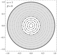
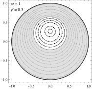
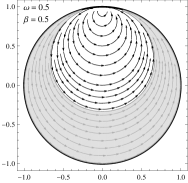
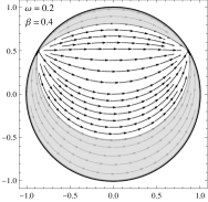
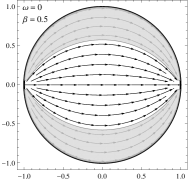
Figure 1: Integral curves (stream lines) of the vector field $v=\omega\xi^{(R)}+\beta\xi^{(B_{1})}$ on the Poincaré disk, for different values of $\omega$ and $\beta$. The white area denotes the physical region, where the fluid velocity does not exceed the speed of light.

In what follows, we shall analyze each of the three distinct cases separately.

3.3.1 Rigid rotation

As was explained above, for $\omega^{2}>\beta^{2}$ one can take $\beta=0$ without loss of generality. The 3-velocity of the fluid is then given by

$$u=\gamma(\partial_{t}+\omega\partial_{\varphi})\,,$$ (40)

where $\omega\in\mathbb{R}$ and $\gamma=(1-\omega^{2}\ell^{2}\sinh^{2}\theta)^{-1/2}$. Note that the flow is well-defined only in the region $U=\{(\theta,\varphi)\,|\,|\omega|\ell\sinh\theta<1\}$. At the boundary of $U$, the fluid rotates at the speed of light. Since $v=\omega\partial_{\varphi}$ is a Killing field of $\text{H}^{2}$, this configuration is shearless and incompressible. The stress tensor is given by

$$T^{\mu\nu}={\cal P}\begin{pmatrix}3\gamma^{2}-1&0&3\gamma^{2}\omega\\ 0&\frac{1}{\ell^{2}}&0\\ 3\gamma^{2}\omega&0&\frac{3\gamma^{2}-2}{\ell^{2}\sinh^{2}\theta}\end{pmatrix}\,,$$ (41)

which is conserved once (24) is satisfied. Moreover, the heat flux $q^{\mu}$ and diffusion current $q^{\mu}_{\text{e}}$ vanish by virtue of propositions 3 and 4.

Since the fluid velocity tends to the speed of light at the boundary of $U$, $\gamma$ diverges there and the total energy and angular momentum are infinite. Thus, unlike in the spherical case, we cannot define global thermodynamical variables here, and have to consider instead only their densities. These are

1. the energy density $\varepsilon=T_{tt}={\cal P}_{0}\gamma^{3}(3\gamma^{2}-1)$,

2. the angular momentum density $l=-T_{t\varphi}=3{\cal P}_{0}\ell^{2}\omega\gamma^{5}\sinh^{2}\theta$,

3. the entropy density $\sigma=J_{S}^{t}=\tau^{2}\gamma^{3}(3h(\psi)-\psi h^{\prime}(\psi))=\gamma s$,

4. the charge density $\varrho_{\text{e}}=J^{t}=\tau^{2}\gamma^{3}h^{\prime}(\psi)=\gamma\rho_{\text{e}}$.

We remark that these densities are evaluated in the frame $(t,\theta,\varphi)$, in which the fluid is moving, while the densities $\rho,s,\rho_{\text{e}}$ are measured in the local rest frame of the fluid. Pointwise, $\varepsilon,l,\sigma$ and $\varrho_{\text{e}}$ are functions of the free parameters $\omega,\tau,\psi$. Calculating their differentials one finds a local form of the first law,

$$\mathrm{d}\varepsilon=\tau\mathrm{d}\sigma+\omega\mathrm{d}l+\tau\psi\mathrm{d}\varrho_{\text{e}}\,,$$ (42)

which implies that the intensive variables conjugate to $\sigma,l$ and $\varrho_{\text{e}}$ are respectively given by

$$\frac{\partial\varepsilon(\sigma,l,\varrho_{\text{e}})}{\partial\sigma}=\tau\,,\qquad\frac{\partial\varepsilon(\sigma,l,\varrho_{\text{e}})}{\partial l}=\omega\,,\qquad\frac{\partial\varepsilon(\sigma,l,\varrho_{\text{e}})}{\partial\varrho_{\text{e}}}=\tau\psi\,.$$ (43)

The local grandcanonical potential $\mathpzc{g}=\varepsilon-\tau\sigma-\omega l-\tau\psi\varrho_{\text{e}}$ reads

$$\mathpzc{g}=-\tau^{3}\gamma^{3}h(\psi)=-\frac{\tau^{3}h(\psi)}{(1-\omega^{2}\ell^{2}\sinh^{2}\theta)^{3/2}}\,.$$ (44)

(42) is of course a consequence of local thermodynamical equilibrium.

3.3.2 Purely translational flow

Now we consider the case $\omega^{2}<\beta^{2}$, in which one can take $\omega=0$ without loss of generality. This flow is visualized in the last figure of 1. In this case it is convenient to use the coordinates

$$X=\sinh\theta\cos\varphi\,,\qquad Y=\sinh\theta\sin\varphi\,,$$ (45)

in which the metric of the spacetime is given by

$$g=-\mathrm{d}t^{2}+\frac{\ell^{2}}{1+X^{2}+Y^{2}}\left((1+Y^{2})\mathrm{d}X^{2}+(1+X^{2})\mathrm{d}Y^{2}-2XY\mathrm{d}X\mathrm{d}Y\right)\,,$$ (46)

and the the fluid moves along the $X$ direction,

$$v=\beta\sqrt{1+X^{2}+Y^{2}}\partial_{X}\,.$$ (47)

Since $v^{2}=\beta^{2}\ell^{2}(1+Y^{2})$, the physical region $U$ is vertically narrowed by the condition

$$Y^{2}<\frac{1}{\beta^{2}\ell^{2}}-1\,,$$ (48)

which also shows that the flow exists only for $\beta^{2}<\ell^{-2}$. The 3-velocity reads

$$u=\gamma(\partial_{t}+\beta\sqrt{1+X^{2}+Y^{2}}\partial_{X})\,,$$ (49)

where $\gamma=(1-\beta^{2}\ell^{2}(1+Y^{2}))^{-1/2}$.

Notice that the lower two figures of 1 look very reminiscent of the black funnels constructed in Fischetti:2012vt to study heat transport in holographic CFT’s. This raises the question whether the bulk duals of the fluid flows in hyperbolic space considered here could be used as toy models for the gravity side of the construction in Fischetti:2012vt . In this context, one should note however that the black funnels of Fischetti:2012vt contain a single connected bulk horizon that extends to meet the conformal boundary. Thus the induced boundary metric has smooth horizons as well. In our case instead, it turns out that the bulk horizon does not extend to meet the boundary, although the boundary metric itself may be considered to contain a horizon, since $\mathbb{R}\times\text{H}^{2}$ is conformal to the static patch of three-dimensional de Sitter space Fischetti:2012vt , which has a cosmological horizon.

3.3.3 Mixed flow: $\omega^{2}=\beta^{2}$

Finally, in the parabolic case $\omega^{2}=\beta^{2}$ one can choose $\omega=\beta$, as was explained above. The Killing vector $v$ becomes then

$$v=\beta\left(iz+\frac{1}{2}(1-z^{2})\right)\partial_{z}+\text{c.c.}$$

It proves useful to introduce new coordinates $A,B$ defined by

$$A=\ln\frac{1-z\bar{z}}{z\bar{z}+i(z-\bar{z})+1}\,,\qquad B=\frac{z+\bar{z}}{z\bar{z}+i(z-\bar{z})+1}\,,$$

such that $v=\beta\partial_{B}$ and

$$g=-\mathrm{d}t^{2}+\ell^{2}(\mathrm{d}A^{2}+e^{-2A}\mathrm{d}B^{2})\,.$$ (50)

The 3-velocity becomes

$$u=\gamma(\partial_{t}+\beta\partial_{B})\,,$$ (51)

with the Lorentz factor $\gamma=(1-\beta^{2}\ell^{2}e^{-2A})^{-1/2}$. The physical region $U$ is thus given by $1-\beta^{2}\ell^{2}e^{-2A}>0$.

3.4 Fluid in rigid rotation on $\text{H}^{2}$ seen on the sphere or plane

The manifolds $\mathbb{R}\times\text{S}^{2}$ and $\mathbb{R}\times\text{H}^{2}$, with metrics (21) and (36), are conformally flat. This means that each of them can be brought by a combined diffeomorphism plus Weyl rescaling into a part of the other or into a part of three-dimensional Minkowski space $\mathbb{M}^{3}$. One might thus ask how a fluid in one of these spaces appears when seen in the others after a conformal transformation. Since one may be interested in the description of hyperbolic AdS black holes in terms of hydrodynamics on Minkowski space or on $\mathbb{R}\times\text{S}^{2}$, we study as an example the rigidly rotating fluid on $\mathbb{R}\times\text{H}^{2}$ analyzed in subsection 3.3.1 to see how it looks like on $\mathbb{M}^{3}$ or on the closed Einstein static universe. We will see that this leads to interesting dynamical fluid configurations.

The coordinate transformation

$$T=\ell e^{\frac{t}{\ell}}\cosh\theta\,,\qquad X=\ell e^{\frac{t}{\ell}}\sinh\theta\cos\varphi\,,\qquad Y=\ell e^{\frac{t}{\ell}}\sinh\theta\sin\varphi\,,$$ (52)

combined with a conformal rescaling $\tilde{g}=\Omega^{2}g$, where

$$\Omega=e^{\frac{t}{\ell}}=\frac{\sqrt{T^{2}-X^{2}-Y^{2}}}{\ell}\,,$$ (53)

brings (36) to the flat metric

$$\tilde{g}=-\mathrm{d}T^{2}+\mathrm{d}X^{2}+\mathrm{d}Y^{2}\,.$$ (54)

Now consider the rigidly rotating fluid in 3.3.1, which has 3-velocity

$$u=\gamma(\partial_{t}+\omega\partial_{\varphi})=\frac{\gamma T}{\ell}\left(\partial_{T}+\frac{X-\omega\ell Y}{T}\partial_{X}+\frac{Y+\omega\ell X}{T}\partial_{Y}\right)\,,$$ (55)

where

$$\gamma=(1-\omega^{2}\ell^{2}\sinh^{2}\theta)^{-\frac{1}{2}}=\sqrt{\frac{T^{2}-X^{2}-Y^{2}}{T^{2}-(1+\omega^{2}\ell^{2})(X^{2}+Y^{2})}}\,.$$ (56)

Recall that the flow is defined only for $|\omega|\ell\sinh\theta<1$. In the coordinates $(T,X,Y)$, this condition becomes $(1+\omega^{2}\ell^{2})(X^{2}+Y^{2})<T^{2}$. Notice also that (52) maps $\mathbb{R}\times\text{H}^{2}$ to the inside of the future light cone $X^{2}+Y^{2}<T^{2}$, $T>0$. The conformal rescaling transforms $u$ into

$$\tilde{u}=\Omega^{-1}u=\frac{T}{\sqrt{T^{2}-(1+\omega^{2}\ell^{2})(X^{2}+Y^{2})}}\left(\partial_{T}+\frac{X-\omega\ell Y}{T}\partial_{X}+\frac{Y+\omega\ell X}{T}\partial_{Y}\right)\,.$$ (57)

This flow is plotted in coordinates $(T,X,Y)$ in figure 2.

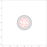
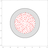
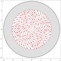
Figure 2: Fluid in rigid rotation on $\text{H}^{2}$ with $\omega=\ell=1$, seen on the plane in coordinates $X,Y$, at times $T=1$, $T=2$ and $T=3$. The grey area is the region of spacetime where the flow is not defined.

We see that the rigidly rotating fluid in $\mathbb{R}\times\text{H}^{2}$ appears in Minkowski space as an expanding vortex.

Let us now transform the same fluid configuration to the closed Einstein static universe $\mathbb{R}\times\text{S}^{2}$. To this aim, introduce new coordinates

$$\tau=-\ell\arctan\frac{\cosh\theta}{\sinh\frac{t}{\ell}}\,,\qquad\Theta=\arctan\frac{\sinh\theta}{\cosh\frac{t}{\ell}}\,,\qquad\Phi=\varphi\,,$$ (58)

where $\tau\in(-\ell\frac{\pi}{2},0)$, $\Theta\in(0,\frac{\pi}{2})$ and $\Phi\in(0,2\pi)$. The inverse of (58) is

$$t=\ell{\mathrm{arsinh}}\frac{\cos\frac{\tau}{\ell}}{\sqrt{\cos^{2}\Theta-\cos^{2}\frac{\tau}{\ell}}}\,,\qquad\theta={\mathrm{arsinh}}\frac{\sin\frac{\tau}{\ell}}{\sqrt{\cos^{2}\Theta-\cos^{2}\frac{\tau}{\ell}}}\,,$$ (59)

hence one has the additional restriction $\Theta<-\frac{\tau}{\ell}$. Subsequently, rescale (36) as $\tilde{g}=\Omega^{2}g$, where

$$\Omega=\sqrt{\cos^{2}\Theta-\cos^{2}\frac{\tau}{\ell}}\,,$$ (60)

to get

$$\tilde{g}=-\mathrm{d}\tau^{2}+\ell^{2}(\mathrm{d}\Theta^{2}+\sin^{2}\Theta\mathrm{d}\Phi^{2})\,.$$ (61)

Now the 3-velocity (40) of the rigidly rotating fluid on $\text{H}^{2}$ is mapped into

$$\tilde{u}=\Omega^{-1}u=\frac{-\sin\frac{\tau}{\ell}\cos\Theta}{\sqrt{\sin^{2}\frac{\tau}{\ell}-(1+\omega^{2}\ell^{2})\sin^{2}\Theta}}\left(\partial_{\tau}+\frac{\tan\Theta}{\ell\tan\frac{\tau}{\ell}}\partial_{\Theta}+\frac{\omega}{-\sin\frac{\tau}{\ell}\cos\Theta}\partial_{\Phi}\right)\,.$$ (62)

In the coordinates $(\tau,\Theta,\Phi)$, the constraint $|\omega|\ell\sinh\theta<1$, limiting the region where the fluid is located, becomes

$$\sin\Theta<\frac{-\sin\frac{\tau}{\ell}}{\sqrt{1+\omega^{2}\ell^{2}}}\,.$$ (63)

This flow is plotted in figure 3 at different times $\tau$ projected on the equatorial plane of $\text{S}^{2}$ and viewed from the north pole.

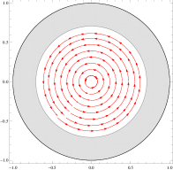
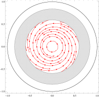
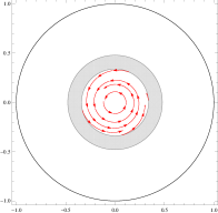
Figure 3: Fluid in rigid rotation on $\text{H}^{2}$ with $\omega=\ell=1$, seen on the 2-sphere (from the north pole and projected on the equatorial plane), at times $\tau\simeq-\ell\frac{\pi}{2}$, $\tau=-\ell$ and $\tau=-\frac{\ell}{2}$. The grey area is the region of spacetime where the flow is not defined.

Again, we encounter a dynamical fluid configuration that is a sort of contracting vortex on $\text{S}^{2}$.

Note that a similar technique was applied in 3+1 dimensions in Gubser:2010ui . There, it was shown (using the Weyl covariance of the stress tensor) that the dynamical solution of Gubser:2010ze (which represents a generalization of Bjorken flow Bjorken:1982qr ) can be recast as a static flow in three-dimensional de Sitter space times a line. The simplicity of the de Sitter form enabled the authors of Gubser:2010ui to obtain several generalizations of it, such as flows in other spacetime dimensions, second order viscous corrections, and linearized perturbations.

4 Dual AdS black holes

Now we want to identify the AdS black holes dual to the fluid configurations classified in section 3. It turns out that these bulk spacetimes are all contained in the Carter-Plebański family Carter:1968ks ; Plebanski:1975 , whose metric is given by

$$\mathrm{d}s^{2}=\frac{p^{2}+q^{2}}{\mathsf{P}(p)}\mathrm{d}p^{2}+\frac{\mathsf{P}(p)}{p^{2}+q^{2}}(\mathrm{d}\tau+q^{2}\mathrm{d}\sigma)^{2}+\frac{p^{2}+q^{2}}{\mathsf{Q}(q)}\mathrm{d}q^{2}-\frac{\mathsf{Q}(q)}{p^{2}+q^{2}}(\mathrm{d}\tau-p^{2}\mathrm{d}\sigma)^{2}\,,$$ (64)

where

$$\mathsf{P}(p)=\alpha-\mathrm{g}^{2}+2lp-\epsilon p^{2}+\frac{p^{4}}{\ell^{2}}\,,\qquad\mathsf{Q}(q)=\alpha+\mathrm{e}^{2}-2mq+\epsilon q^{2}+\frac{q^{4}}{\ell^{2}}\,.$$ (65)

This solves the Einstein-Maxwell equations with cosmological constant $\Lambda=-3\ell^{-2}$ and electromagnetic field

$$A=-\frac{\mathrm{e}\,q}{p^{2}+q^{2}}(\mathrm{d}\tau-p^{2}\mathrm{d}\sigma)-\frac{\mathrm{g}\,p}{p^{2}+q^{2}}(\mathrm{d}\tau+q^{2}\mathrm{d}\sigma)\,,$$ (66)

whose field strength is

$$F=\frac{\mathrm{e}(p^{2}-q^{2})+2\mathrm{g}\,pq}{(p^{2}+q^{2})^{2}}\mathrm{d}q\wedge(\mathrm{d}\tau-p^{2}\mathrm{d}\sigma)-\frac{\mathrm{g}(p^{2}-q^{2})-2\mathrm{e}\,pq}{(p^{2}+q^{2})^{2}}\mathrm{d}p\wedge(\mathrm{d}\tau+q^{2}\mathrm{d}\sigma)\,.$$ (67)

(64) can be obtained by a scaling limit from the Plebański-Demiański spacetime Plebanski:1976gy , which is the most general known Petrov-type D solution to the Einstein-Maxwell equations with cosmological constant. Other references studying algebraically special spacetimes and their fluid duals include deFreitas:2014lia , where the AdS/CFT interpretation of the Robinson-Trautman (RT) solution to vacuum AdS gravity was investigated. This is slightly different from our case, since the boundary metric of the RT geometry is in general time-dependent deFreitas:2014lia .

The metric $\hat{g}$ on the conformal boundary of (64) can be obtained by setting $q=\text{const.}\to\infty$ and rescaling with $\ell^{2}/q^{2}$. This leads to

$${\hat{g}}=-\mathrm{d}\tau^{2}+\frac{\ell^{2}}{\mathsf{P}(p)}\mathrm{d}p^{2}+(\ell^{2}\mathsf{P}(p)-p^{4})\mathrm{d}\sigma^{2}+2p^{2}\mathrm{d}\tau\mathrm{d}\sigma\,.$$ (68)

Notice that for vanishing NUT-parameter $l$ this metric is conformally flat. In what follows, we shall consider the case $l=0$ only.

Using standard holographic renormalization techniques Balasubramanian:1999re , one can compute the holographic stress tensor associated to (64), with the result

$$\hat{T}_{\mu\nu}=\frac{m}{8\pi\ell^{2}}(\gamma_{\mu\nu}+3u_{\mu}u_{\nu})\,,$$ (69)

where $u=\partial_{\tau}$. $\hat{T}$ describes thus a conformal fluid in equilibrium, at rest in the frame $(\tau,p,\sigma)$. The external electromagnetic field $\hat{F}$ and the $\text{U}(1)$ current $\hat{J}$ dual to (66) on the conformal boundary of (64) are found to be respectively

$$\hat{F}=\mathrm{g}\,\mathrm{d}p\wedge\mathrm{d}\sigma\,,\qquad\hat{J}=\frac{\mathrm{e}}{4\pi\ell^{2}}\partial_{\tau}=\frac{\mathrm{e}}{4\pi\ell^{2}}u\,.$$ (70)

The last equation shows that the fluid has a constant charge density $\mathrm{e}/(4\pi\ell^{2})$. Note also that the current $\hat{J}$ is conserved, ${\hat{\nabla}}_{\mu}\hat{J}^{\mu}=0$, where $\hat{\nabla}$ denotes the Levi-Civita connection of $\hat{g}$. Moreover, since $\hat{F}_{\mu\nu}\hat{J}^{\nu}=0$, the Lorentz force exerted by the field $\hat{F}$ on the charged fluid vanishes, and thus $\hat{T}$ is conserved as well, ${\hat{\nabla}}_{\mu}\hat{T}^{\mu\nu}=0$.

Notice that the solution (64), (67) enjoys the scaling symmetry

$$p\to\lambda p\,,\qquad q\to\lambda q\,,\qquad\tau\to\tau/\lambda\,,\qquad\sigma\to\sigma/\lambda^{3}\,,\qquad\alpha\to\lambda^{4}\alpha\,,$$

$$\mathrm{g}\to\lambda^{2}\mathrm{g}\,,\qquad\mathrm{e}\to\lambda^{2}\mathrm{e}\,,\qquad m\to\lambda^{3}m\,,\qquad l\to\lambda^{3}l\,,\qquad\epsilon\to\lambda^{2}\epsilon\,,$$ (71)

that can be used to eliminate one unphysical parameter.

The line element (64) describes a black hole whose event horizon $\cal H$ is located at the largest root of the polynomial $\mathsf{Q}(q)$. As we shall see below, the horizon geometry depends crucially on the choice of parameters contained in the function $\mathsf{P}(p)$, which determine the number of real roots of $\mathsf{P}$. In what follows, we will discuss more in detail some subcases of the Carter-Plebański family, which are dual to the fluid configurations classified in section 3.

4.1 Spherical and hyperbolic Kerr-Newman-AdS₄ black holes

If we set

$$\alpha=ka^{2}+\mathrm{g}^{2}\,,\quad\epsilon=k+\frac{a^{2}}{\ell^{2}}\,,\quad\tau=\frac{t-a\varphi}{\Xi}\,,\quad q=r\,,\quad p=ac_{k}(\theta)\,,\quad\sigma=-\frac{\varphi}{a\Xi}\,,$$

where

$$k=\pm 1\,,\qquad\Xi=1-\frac{ka^{2}}{\ell^{2}}\,,\qquad c_{k}(\theta)=\frac{ds_{k}(\theta)}{d\theta}\,,\qquad s_{k}(\theta)=\left\{\begin{matrix}\sin\theta\,,\quad k=1\,,\\ \sinh\theta\,,\quad k=-1\,,\end{matrix}\right.$$

the metric (64) becomes

$$\mathrm{d}s^{2}=-\frac{\Delta_{r}}{\Xi^{2}\rho^{2}}\left(\mathrm{d}t-ka\,s_{k}^{2}(\theta)\mathrm{d}\varphi\right)^{2}+\rho^{2}\left(\frac{\mathrm{d}r^{2}}{\Delta_{r}}+\frac{\mathrm{d}\theta^{2}}{\Delta_{\theta}}\right)+\frac{\Delta_{\theta}}{\Xi^{2}\rho^{2}}\left(a\mathrm{d}t-(r^{2}+a^{2})\mathrm{d}\varphi\right)^{2}s_{k}^{2}(\theta)\,,$$ (72)

with

$$\rho^{2}=r^{2}+a^{2}c_{k}^{2}(\theta)\,,\qquad\Delta_{r}=(r^{2}+a^{2})\left(k+\frac{r^{2}}{\ell^{2}}\right)-2mr+\mathrm{e}^{2}+\mathrm{g}^{2}\,,\qquad\Delta_{\theta}=1-\frac{ka^{2}}{\ell^{2}}c_{k}^{2}(\theta)\,.$$

For $k=1$ this is the Kerr-Newman-AdS₄ black hole, while for $k=-1$ one has the rotating hyperbolic solution constructed in Klemm:1997ea . Note also that in the spherical case $(k=1)$ the rotation parameter $a$ is bounded by $a^{2}<\ell^{2}$ in order for $\Delta_{\theta}$ to be positive, while it can take any value if $k=-1$.

The metric on the conformal boundary of (72) reads

$${\hat{g}}=-\frac{\mathrm{d}t^{2}}{\Xi^{2}}+\frac{\ell^{2}\mathrm{d}\theta^{2}}{\Delta_{\theta}}+\frac{\ell^{2}}{\Xi}s_{k}^{2}(\theta)\mathrm{d}\varphi^{2}+2\frac{ak}{\Xi^{2}}s_{k}^{2}(\theta)\mathrm{d}t\mathrm{d}\varphi\,.$$ (73)

Since this is conformally flat there exist coordinates in which, after a conformal rescaling, it takes the ultrastatic spherical or hyperbolic form (like in eqns. (21) and (36)). These are given by

$$\tau=\frac{t}{\Xi}\,,\qquad c_{k}(\Theta)=c_{k}(\theta)\sqrt{\frac{\Xi}{\Delta_{\theta}}}\,,\qquad\Phi=\varphi+\frac{kat}{\ell^{2}\Xi}\,.$$ (74)

Notice that $\Theta$ ranges in $(0,\pi)$ when $k=1$ and in $(0,\text{arsinh}(\ell/|a|))$ when $k=-1$, cf. fig. 4, where $\Theta(\theta)$ is plotted for different values of $a/\ell$.

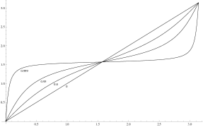
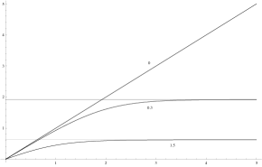
Figure 4: Graphs of $\Theta(\theta)$ for $k=1$ (left) and $k=-1$ (right), for different values of $a/\ell$.

In the new coordinates, the boundary metric (73) takes the form

$${\hat{g}}=\frac{\Delta_{\theta}}{\Xi}\left(-\mathrm{d}\tau^{2}+\ell^{2}(\mathrm{d}\Theta^{2}+s_{k}^{2}(\Theta)\mathrm{d}\Phi^{2})\right)\,,$$ (75)

such that, after a Weyl rescaling

$${\hat{g}}\rightarrow\tilde{g}=\Omega^{2}{\hat{g}}\,,\qquad\Omega^{2}=\Xi/\Delta_{\theta}\,,$$ (76)

one obtains the desired metric

$$\tilde{g}=-\mathrm{d}\tau^{2}+\ell^{2}(\mathrm{d}\Theta^{2}+s_{k}^{2}(\Theta)\mathrm{d}\Phi^{2})\,.$$ (77)

Thus the boundary of the Kerr-AdS₄ black hole is conformal to $\mathbb{R}\times\text{S}^{2}$ for $k=1$, and to the part of $\mathbb{R}\times\text{H}^{2}$ with $\sinh\Theta<\ell/|a|$ for $k=-1$. If we identify $|\omega|=|a|/\ell^{2}$, this is exactly the part of $\mathbb{R}\times\text{H}^{2}$ on which a fluid in rigid rotation with angular velocity $\omega$ does not exceed the speed of light. We will have to say more on this below.

The holographic stress tensor associated to (72) can be written in the form

$$\hat{T}_{\mu\nu}=\frac{m}{8\pi\ell^{2}}\left({\hat{g}}_{\mu\nu}+3u_{\mu}u_{\nu}\right)\,,$$ (78)

where $u=\Xi\partial_{t}$. This is the stress tensor of a conformal fluid at rest in the coordinate frame $(t,\theta,\varphi)$, with pressure ${\cal P}=m/(8\pi\ell^{2})$. After the diffeomorphism (74) and the subsequent Weyl rescaling (76) (recall that $\hat{T}$ transforms as $\tilde{T}^{\mu\nu}=\Omega^{-d-2}\hat{T}^{\mu\nu}$) one obtains

$$\tilde{T}^{\mu\nu}=\frac{m\gamma^{3}}{8\pi\ell^{2}}\begin{pmatrix}3\gamma^{2}-1&0&\frac{3ka\gamma^{2}}{\ell^{2}}\\ 0&\frac{1}{\ell^{2}}&0\\ \frac{3ka\gamma^{2}}{\ell^{2}}&0&\frac{3\gamma^{2}-2}{\ell^{2}s_{k}^{2}(\Theta)}\end{pmatrix}\,,$$ (79)

with $\gamma:=(1-a^{2}s_{k}^{2}(\Theta)/\ell^{2})^{-1/2}$. This can also be rewritten as $\tilde{T}^{\mu\nu}=\tilde{\cal P}\left(\tilde{g}^{\mu\nu}+3\tilde{u}^{\mu}\tilde{u}^{\nu}\right)$, where

$$\tilde{\cal P}=\Omega^{-3}{\cal P}=\frac{m\gamma^{3}}{8\pi\ell^{2}}\,,\qquad\tilde{u}=\Omega^{-1}u=\gamma(\partial_{\tau}+\frac{ka}{\ell^{2}}\partial_{\Phi})\,.$$ (80)

For $k=1$, $\tilde{T}$ is exactly the stress tensor (23) of the stationary conformal fluid on the 2-sphere, if we identify

$${\cal P}_{0}=\frac{m}{8\pi\ell^{2}}\,,\qquad\omega=\frac{a}{\ell^{2}}\,.$$ (81)

On the other hand, for $k=-1$, (79) coincides with the stress tensor (41) of the rigidly rotating conformal fluid on the hyperbolic plane, after the identifications

$${\cal P}_{0}=\frac{m}{8\pi\ell^{2}}\,,\qquad\omega=-\frac{a}{\ell^{2}}\,.$$ (82)

The KNAdS black hole is thus dual to a fluid in rigid rotation on $\text{S}^{2}$ for $k=1$ and on $\text{H}^{2}$ for $k=-1$. In the spherical case, this is of course well-known Bhattacharyya:2007vs ; Caldarelli:2008ze . The result for hyperbolic black holes is new, and it is remarkable how the conformal transformation (74), (76) maps the boundary geometry of the rotating hyperbolic black hole precisely to the region of $\mathbb{R}\times\text{H}^{2}$ on which a fluid in rigid rotation does not exceed the speed of light.

The electromagnetic field and electric current on the boundary are given respectivey by

$$\hat{F}=\frac{k\mathrm{g}s_{k}(\theta)}{\Xi}\mathrm{d}\theta\wedge\mathrm{d}\varphi\,,\qquad\hat{J}=\frac{\mathrm{e}\Xi}{4\pi\ell^{2}}\partial_{t}=\frac{\mathrm{e}}{4\pi\ell^{2}}u\,.$$ (83)

After the coordinate change (74) and Weyl rescaling (76), they become

$$\tilde{F}=k\mathrm{g}\gamma^{3}s_{k}(\Theta)\,\mathrm{d}\Theta\wedge(\mathrm{d}\Phi-\frac{ka}{\ell^{2}}\mathrm{d}\tau)\,,\qquad\tilde{J}=\frac{\mathrm{e}\gamma^{3}}{4\pi\ell^{2}}(\partial_{\tau}+\frac{ka}{\ell^{2}}\partial_{\Phi})=\frac{\mathrm{e}\gamma^{2}}{4\pi\ell^{2}}\tilde{u}\,,$$ (84)

and thus $\tilde{J}$ coincides with the hydrodynamical expression if the charge density of the fluid is

$$\rho_{\text{e}}=\frac{\mathrm{e}\gamma^{2}}{4\pi\ell^{2}}\,.$$ (85)

Note that in the coordinate system $(\tau,\Theta,\Phi)$ there is also an electric field. Moreover, one has $\tilde{F}^{\nu}{}_{\mu}\tilde{J}^{\mu}=0$, so there is no net Lorentz force acting on the charged fluid due to an exact cancellation of electric and magnetic forces. In the orthonormal frame

$$e^{0}=\mathrm{d}\tau\,,\qquad e^{1}=\ell\mathrm{d}\Theta\,,\qquad e^{2}=\ell s_{k}(\Theta)\mathrm{d}\Phi\,,$$

the electric field in $1$-direction and the spatial current in $2$-direction are

$$E^{1}=\frac{\mathrm{g}\gamma^{3}s_{k}(\Theta)a}{\ell^{3}}\,,\qquad\tilde{J}^{\,2}=\frac{\mathrm{e}\gamma^{3}s_{k}(\Theta)ka}{4\pi\ell^{3}}=\sigma^{21}E^{1}\,,$$ (86)

with the Hall conductivity

$$\sigma^{21}=\frac{\mathrm{e}k}{4\pi\mathrm{g}}\,.$$ (87)

In the spherical case $k=1$, it was furthermore shown in Bhattacharyya:2007vs that, in the large black hole limit where fluid dynamics provides an accurate description of the dual conformal field theory, the black hole electric charge, entropy, mass and angular momentum coincide precisely with the conserved charges (25), (26) and (27) computed in fluid mechanics, if we identify the Hawking temperature $T$ with the global fluid temperature in (29).

On the other hand, for $k=-1$, we already saw in the previous section that the conserved charges are ill-defined in fluid mechanics. The same problem is encountered on the gravity side: If one tries to compute for instance the entropy of the solution (72) with $k=-1$, one has to integrate over the noncompact variable $\theta$, which makes the result divergent. A possible way out could be to consider only excitations above some ‘ground state’, which may have finite energy, but we shall not attempt to do this here. In spite of these difficulties, we saw in section 3.3.1 that a local form of the first law of black hole mechanics holds.

4.2 Boosting AdS₄ black holes

In the previous subsection it was shown that the spherical and hyperbolic KNAdS₄ black holes are holographically dual to conformal fluids in rigid rotation on $\mathbb{R}\times\text{S}^{2}$ and $\mathbb{R}\times\text{H}^{2}$ respectively. While a rigid rotation is (up to isometries) the only possible equilibrium configuration for a stationary conformal fluid on a sphere, the same is not true for hyperbolic space: We saw in 3.3 that on the hyperbolic plane one can also have purely translational (‘boosting’) or mixed flows, which are not isometric to rotations. In this section we describe a family of black holes, obtained by analytically continuing the hyperbolic KNAdS₄ metric, whose dual fluid is translating on the hyperbolic plane. We will call these solutions ‘boosting black holes’.

Consider the KNAdS₄ metric (72) with $k=-1$, and analytically continue

$$a\rightarrow ib\,,\qquad\theta\rightarrow\theta-\frac{i\pi}{2}\,,\qquad\varphi\rightarrow i\varphi\,.$$ (88)

This leads to

$$\mathrm{d}s^{2}=-\frac{\Delta_{r}}{\Xi^{2}\rho^{2}}\left(\mathrm{d}t+b\cosh^{2}\theta\mathrm{d}\varphi\right)^{2}+\rho^{2}\left(\frac{\mathrm{d}r^{2}}{\Delta_{r}}+\frac{\mathrm{d}\theta^{2}}{\Delta_{\theta}}\right)+\frac{\Delta_{\theta}\cosh^{2}\theta}{\Xi^{2}\rho^{2}}\left(b\mathrm{d}t-(r^{2}-b^{2})\mathrm{d}\varphi\right)^{2}\,,$$ (89)

where now

$$\rho^{2}=r^{2}+b^{2}\sinh^{2}\theta\,,\quad\Delta_{r}=(r^{2}-b^{2})\left(-1+\frac{r^{2}}{\ell^{2}}\right)-2mr+\mathrm{e}^{2}+\mathrm{g}^{2}\,,\quad\Delta_{\theta}=1+\frac{b^{2}}{\ell^{2}}\sinh^{2}\theta\,,$$

and $\Xi=1-b^{2}/\ell^{2}$. Alternatively, (89) can be obtained directly from the Carter-Plebański solution (64) by setting

$$\alpha=b^{2}+\mathrm{g}^{2}\,,\quad l=0\,,\quad\epsilon=-1-\frac{b^{2}}{\ell^{2}}\,,\quad\tau=\frac{t+b\varphi}{\Xi}\,,\quad q=r\,,\quad p=b\sinh\theta\,,\quad\sigma=-\frac{\varphi}{b\Xi}\,.$$

The electromagnetic 1-form potential (66) becomes then

$$A=-\frac{\mathrm{e}r}{\Xi\rho^{2}}\left(\mathrm{d}t+b\cosh^{2}\theta\mathrm{d}\varphi\right)-\frac{\mathrm{g}\sinh\theta}{\Xi\rho^{2}}\left(b\mathrm{d}t-(r^{2}-b^{2})\mathrm{d}\varphi\right)\,.$$ (90)

Notice that now $\theta,\varphi$ are not polar coordinates on $\text{H}^{2}$ (in that case it would not be possible to extend the 1-form $\cosh\theta\,\mathrm{d}\varphi$ to $\theta=0$), but they are rather Cartesian-type coordinates on a plane, possibly compactified to a cylinder by periodic identifications of $\varphi$.

The metric on the conformal boundary of (89) is given by

$${\hat{g}}=-\frac{\mathrm{d}t^{2}}{\Xi^{2}}+\frac{\ell^{2}}{\Delta_{\theta}}\mathrm{d}\theta^{2}+\frac{\ell^{2}}{\Xi}\cosh^{2}\theta\mathrm{d}\varphi^{2}-2\frac{b}{\Xi^{2}}\cosh^{2}\theta\mathrm{d}t\mathrm{d}\varphi\,,$$ (91)

from which we see that $\partial_{\varphi}$ is spacelike only for $b^{2}<\ell^{2}$. Now introduce the ultrastatic coordinates

$$T=\frac{t}{\Xi}\,,\qquad X=\frac{\cosh\theta}{\sqrt{\Delta_{\theta}}}\sinh\left(\varphi-\frac{bt}{\ell^{2}\Xi}\right)\,,\qquad Y=\sqrt{\frac{\Xi}{\Delta_{\theta}}}\sinh\theta\,,$$ (92)

where $T,X\in\mathbb{R}$ and $Y$ is bounded by $Y^{2}<\ell^{2}/b^{2}-1$, and perform a Weyl rescaling $\tilde{g}=\Omega^{2}{\hat{g}}$ with

$$\Omega=\sqrt{\frac{\Xi}{\Delta_{\theta}}}=\sqrt{1-\frac{b^{2}}{\ell^{2}}(1+Y^{2})}\,.$$ (93)

This yields

$$\tilde{g}=-\mathrm{d}T^{2}+\frac{\ell^{2}}{1+X^{2}+Y^{2}}\left((1+Y^{2})\mathrm{d}X^{2}+(1+X^{2})\mathrm{d}Y^{2}-2XY\mathrm{d}X\mathrm{d}Y\right)\,,$$ (94)

which is the slice $Y^{2}<\ell^{2}/b^{2}-1$ of the spacetime $\mathbb{R}\times\text{H}^{2}$, cf. (46).

In the frame $(t,\theta,\varphi)$ the holographic stress tensor on the conformal boundary is found to be

$$\hat{T}_{\mu\nu}=\frac{m}{8\pi\ell^{2}}\left(\gamma_{\mu\nu}+3u_{\mu}u_{\nu}\right)\,,$$ (95)

with $u=\Xi\partial_{t}$. After the diffeomorphism (92) and the Weyl rescaling (93), the stress tensor becomes

$$\tilde{T}_{\mu\nu}=\tilde{\cal P}\left(\tilde{g}_{\mu\nu}+3\tilde{u}_{\mu}\tilde{u}_{\nu}\right)\,,$$ (96)

where

$$\tilde{\cal P}=\frac{m\gamma^{3}}{8\pi\ell^{2}}\,,\qquad\tilde{u}=\gamma\left(\partial_{T}-\frac{b}{\ell^{2}}\sqrt{1+X^{2}+Y^{2}}\partial_{X}\right)\,,\qquad\gamma=\Omega^{-1}=\left(1-\frac{b^{2}}{\ell^{2}}(1+Y^{2})\right)^{-1/2}\,.$$

This is exactly the energy-momentum tensor and 3-velocity of a conformal fluid translating on the hyperbolic plane studied in section 3.3.2, after the identifications

$${\cal P}_{0}=\frac{m}{8\pi\ell^{2}}\,,\qquad\beta=-\frac{b}{\ell^{2}}\,.$$ (97)

The gravity dual of the ‘boosting’ fluid on $\text{H}^{2}$ is thus given by the black hole solution (89), (90). Although the latter is contained in the general Carter-Plebańksi solution, it is in principle new, since its physical properties have not been discussed in the literature so far. Note again the remarkable fact that the conformal transformation (92), (93) maps the boundary geometry of (89) precisely to the region of $\mathbb{R}\times\text{H}^{2}$ in which the fluid velocity does not exceed the speed of light.

4.3 Black holes dual to mixed (parabolic) flow on the hyperbolic plane

Consider now the following choice for the parameters and coordinates of the Carter-Plebański solution (64):

$$\alpha=\mathrm{g}^{2}\,,\qquad l=0\,,\qquad\epsilon=-1\,,\qquad q=r\,,\qquad p=aP\,,\qquad\sigma=-\frac{\varphi}{a}\,,$$

which leads to

$$\mathrm{d}s^{2}=-\frac{\Delta_{r}}{\rho^{2}}\left(\mathrm{d}\tau+aP^{2}\mathrm{d}\varphi\right)^{2}+\rho^{2}\left(\frac{\mathrm{d}r^{2}}{\Delta_{r}}+\frac{\mathrm{d}P^{2}}{\Delta_{P}}\right)+\frac{\Delta_{P}}{\rho^{2}}\left(a\mathrm{d}\tau-r^{2}\mathrm{d}\varphi\right)^{2}\,,$$ (98)

$$A=-\frac{\mathrm{e}r}{\rho^{2}}\left(\mathrm{d}\tau+aP^{2}\mathrm{d}\varphi\right)-\frac{\mathrm{g}P}{\rho^{2}}\left(a\mathrm{d}\tau-r^{2}\mathrm{d}\varphi\right)\,,$$ (99)

where

$$\rho^{2}=r^{2}+a^{2}P^{2}\,,\qquad\Delta_{r}=r^{2}\left(\frac{r^{2}}{\ell^{2}}-1\right)-2mr+\mathrm{e}^{2}+\mathrm{g}^{2}\,,\qquad\Delta_{P}=P^{2}\left(1+\frac{a^{2}}{\ell^{2}}P^{2}\right)\,.$$

The metric on the conformal boundary of (98) reads

$${\hat{g}}=-\mathrm{d}\tau^{2}+\frac{\ell^{2}}{\Delta_{P}}\mathrm{d}P^{2}+\ell^{2}P^{2}\mathrm{d}\varphi^{2}-2aP^{2}\mathrm{d}\tau\mathrm{d}\varphi\,,$$ (100)

and the holographic stress tensor takes the usual form

$$\hat{T}_{\mu\nu}=\frac{m}{8\pi\ell^{2}}\left({\hat{g}}_{\mu\nu}+3u_{\mu}u_{\nu}\right)\,,$$ (101)

with 3-velocity $u=\partial_{\tau}$. Like in the previous cases, one can introduce ultrastatic coordinates on the conformal boundary, defined by

$$T=\tau\,,\qquad A=\frac{1}{2}\ln\frac{\Delta_{P}}{P^{4}}\,,\qquad B=\varphi-\frac{a\tau}{\ell^{2}}\,,$$ (102)

where $A>\frac{1}{2}\ln\frac{a^{2}}{\ell^{2}}$ and $T,B\in\mathbb{R}$. After a subsequent Weyl rescaling $\tilde{g}=\Omega^{2}{\hat{g}}$ with

$$\Omega=\frac{P}{\sqrt{\Delta_{P}}}=\sqrt{1-\frac{a^{2}}{\ell^{2}}e^{-2A}}\,,$$ (103)

one gets the metric

$$\tilde{g}=-\mathrm{d}T^{2}+\ell^{2}(\mathrm{d}A^{2}+e^{-2A}\mathrm{d}B^{2})\,.$$ (104)

Thus we have shown that the boundary geometry of (98) is conformal to the subset $A>\frac{1}{2}\ln\frac{a^{2}}{\ell^{2}}$ of the spacetime $\mathbb{R}\times\text{H}^{2}$. After the coordinate transformation (102) and the Weyl rescaling (103), the 3-velocity $u$ becomes

$$\tilde{u}=\gamma(\partial_{T}-\frac{a}{\ell^{2}}\partial_{B})\,,$$ (105)

where

$$\gamma=\Omega^{-1}=\left(1-\frac{a^{2}}{\ell^{2}}e^{-2A}\right)^{-1/2}\,.$$ (106)

The transformed energy-momentum tensor $\tilde{T}$ and the 3-velocity $\tilde{u}$ coincide with the ones considered in section 3.3.3, if we identify

$${\cal P}_{0}=\frac{m}{8\pi\ell^{2}}\,,\qquad\beta=-\frac{a}{\ell^{2}}\,.$$ (107)

The gravity dual of the mixed (parabolic) flow on $\text{H}^{2}$ is thus given by the black hole solution (98). Again, the conformal transformation (102), (103) maps the boundary of (98) exactly to the region $1-\beta^{2}\ell^{2}e^{-2A}>0$ where the fluid velocity is smaller than the speed of light. If $\varphi$ is compactified, $B$ becomes also a compact coordinate. The flow in this case is visualized in fig. 5.

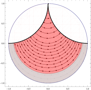
Figure 5: Poincaré disk compactified by identifications of the coordinate $B$; the two thick black lines have to be identified. The grey area is the unphysical region where the fluid velocity exceeds the speed of light. The fluid is located in the red region.

4.4 Black holes dual to rotating fluid on the Euclidean plane

The family of black holes dual to a rotating fluid in Minkowski space $\mathbb{R}\times\text{E}^{2}$ is obtained by making the following choice for the parameters and coordinates of the Carter-Plebański solution (64):

$$\alpha=\mathrm{g}^{2}\,,\qquad l=0\,,\qquad\epsilon=\frac{a^{2}}{\ell^{2}}\,,\qquad q=r\,,\qquad p=aP\,,\qquad\sigma=-\frac{\varphi}{a}\,,$$

which leads to

$$\mathrm{d}s^{2}=-\frac{\Delta_{r}}{\rho^{2}}\left(\mathrm{d}\tau+aP^{2}\mathrm{d}\varphi\right)^{2}+\rho^{2}\left(\frac{\mathrm{d}r^{2}}{\Delta_{r}}+\frac{\mathrm{d}P^{2}}{\Delta_{P}}\right)+\frac{\Delta_{P}}{\rho^{2}}\left(a\mathrm{d}\tau-r^{2}\mathrm{d}\varphi\right)^{2}\,,$$ (108)

$$A=-\frac{\mathrm{e}r}{\rho^{2}}\left(\mathrm{d}\tau+aP^{2}\mathrm{d}\varphi\right)-\frac{\mathrm{g}P}{\rho^{2}}\left(a\mathrm{d}\tau-r^{2}\mathrm{d}\varphi\right)\,,$$ (109)

where

$$\rho^{2}=r^{2}+a^{2}P^{2}\,,\qquad\Delta_{r}=\frac{r^{2}}{\ell^{2}}(r^{2}+a^{2})-2mr+\mathrm{e}^{2}+\mathrm{g}^{2}\,,\qquad\Delta_{P}=\frac{a^{2}}{\ell^{2}}P^{2}(P^{2}-1)\,,$$

and $P>1$. In the uncharged case ($\mathrm{e}=\mathrm{g}=0$), the solution (108) appeared in (C.10) of Mukhopadhyay:2013gja . Notice that, unlike in the previous cases, the Killing vector $\partial_{\varphi}$ becomes timelike for large $r$. Hence, to avoid closed timelike curves, we shall not compactify $\varphi$. Instead we replace the coordinates $\tau,\varphi$ with $T,\Phi$ defined by

$$T=\tau+a\varphi\,,\qquad\Phi=\frac{a\tau}{\ell^{2}}\,.$$ (110)

Since $\partial_{\Phi}$ is spacelike everywhere outside the horizon (located at the largest root of $\Delta_{r}$), we compactify $\Phi\sim\Phi+2\pi$. This choice is done in order that the conformal boundary has the topology of $\mathbb{R}$ times a disk, as we will see shortly.

The boundary geometry of (108) is given by

$${\hat{g}}=-\mathrm{d}\tau^{2}+\frac{\ell^{2}}{\Delta_{P}}\mathrm{d}P^{2}-a^{2}P^{2}\mathrm{d}\varphi^{2}-2aP^{2}\mathrm{d}\tau\mathrm{d}\varphi\,,$$ (111)

and the holographic stress tensor has the usual form (101), where $u=\partial_{\tau}$. Now consider the coordinate transformation (110), supplemented by

$$R=\frac{\ell^{2}}{a}\sqrt{1-P^{-2}}\,,\qquad 0<R<\frac{\ell^{2}}{a}\,,$$ (112)

and perform a Weyl rescaling $\tilde{g}=\Omega^{2}{\hat{g}}$ with

$$\Omega=P^{-1}=\sqrt{1-\frac{a^{2}R^{2}}{\ell^{4}}}\,.$$ (113)

This yields the metric

$$\tilde{g}=-\mathrm{d}T^{2}+\mathrm{d}R^{2}+R^{2}\mathrm{d}\Phi^{2}\,.$$ (114)

Thus we have shown that the conformal boundary is the subset $R<\ell^{2}/a$ of the spacetime $\mathbb{R}\times\text{E}^{2}$, i.e., the real line times a disk. After the coordinate change to $(T,R,\Phi)$ and the conformal rescaling (113), the energy momentum tensor becomes

$$\tilde{T}^{\mu\nu}=\tilde{\cal P}\left(\tilde{g}^{\mu\nu}+3\tilde{u}^{\mu}\tilde{u}^{\nu}\right)\,,$$ (115)

where

$$\tilde{\cal P}=\frac{m\gamma^{3}}{8\pi\ell^{2}}\,,\qquad\tilde{u}=\gamma\left(\partial_{T}+\frac{a}{\ell^{2}}\partial_{\Phi}\right)\,,\qquad\gamma=\Omega^{-1}=\left(1-\frac{a^{2}R^{2}}{\ell^{4}}\right)^{-1/2}\,.$$

The stress tensor (115) and the 3-velocity $\tilde{u}$ coincide with the ones considered in section 3.2, if we identify

$${\cal P}_{0}=\frac{m}{8\pi\ell^{2}}\,,\qquad\omega=\frac{a}{\ell^{2}}\,.$$ (116)

The gravity dual of the rotating fluid on $\text{E}^{2}$ is thus given by the black hole solution (108), and the conformal transformation that we used here maps the boundary geometry of (108) to a line times the disk $R<\ell^{2}/a$, where the fluid flow is well-defined.

4.5 Super-rotating hyperbolic black holes

We saw in section 4.1 that the spherical KNAdS black hole is dual to a rotating fluid on $\text{S}^{2}$ if the angular velocity of the latter is limited by $|\omega|\ell<1$, which translates on the gravity side into $a^{2}<\ell^{2}$. For $|\omega|\ell>1$ the constraint $v^{2}<1$ restricts the rotating fluid to the polar caps $|\omega|\ell\sin\theta<1$. It turns out that in this case the dual black hole can be obtained from the KNAdS₄ metric (72) with $k=1$ by the analytical continuation $\theta\rightarrow i\theta$, which leads to

$$\mathrm{d}s^{2}=-\frac{\Delta_{r}}{\Xi^{2}\rho^{2}}\left(\mathrm{d}t+a\sinh^{2}\theta\mathrm{d}\varphi\right)^{2}+\rho^{2}\left(\frac{\mathrm{d}r^{2}}{\Delta_{r}}+\frac{\mathrm{d}\theta^{2}}{\Delta_{\theta}}\right)+\frac{\Delta_{\theta}\sinh^{2}\theta}{\Xi^{2}\rho^{2}}\left(a\mathrm{d}t-(r^{2}+a^{2})\mathrm{d}\varphi\right)^{2}\,,$$ (117)

$$A=-\frac{\mathrm{e}r}{\Xi\rho^{2}}\left(\mathrm{d}t+a\sinh^{2}\theta\mathrm{d}\varphi\right)-\frac{\mathrm{g}\cosh\theta}{\Xi\rho^{2}}\left(a\mathrm{d}t-(r^{2}+a^{2})\mathrm{d}\varphi\right)\,,$$ (118)

where

$$\rho^{2}=r^{2}+a^{2}\cosh^{2}\theta\,,\quad\Delta_{r}=(r^{2}+a^{2})\left(1+\frac{r^{2}}{\ell^{2}}\right)-2mr+\mathrm{e}^{2}+\mathrm{g^{2}}\,,\quad\Delta_{\theta}=\frac{a^{2}}{\ell^{2}}\cosh^{2}\theta-1\,,$$

and $\Xi=a^{2}/\ell^{2}-1$. Note that there is a lower bound on the rotation parameter $a$: Positivity of $\Delta_{\theta}$ requires $a^{2}>\ell^{2}$, so that these black holes exist only above some minimum amount of rotation and thus have no static limit.

The metric (117) is again a special case of the Carter-Plebański family, obtained by setting

$$\gamma=a^{2}+\mathrm{g}^{2}\,,\quad l=0\,,\quad\epsilon=1+\frac{a^{2}}{\ell^{2}}\,,\quad\tau=\frac{t-a\varphi}{\Xi}\,,\quad q=r\,,\quad p=a\cosh\theta\,,\quad\sigma=-\frac{\varphi}{a\Xi}\,.$$

The metric on the conformal boundary of (117) is given by

$${\hat{g}}=-\frac{\mathrm{d}t^{2}}{\Xi^{2}}+\frac{\ell^{2}}{\Delta_{\theta}}\mathrm{d}\theta^{2}+\frac{\ell^{2}}{\Xi}\sinh^{2}\theta\mathrm{d}\varphi^{2}-\frac{2a}{\Xi^{2}}\sinh^{2}\theta\mathrm{d}t\mathrm{d}\varphi\,.$$ (119)

Now introduce new coordinates $\tau,\Theta,\Phi$ defined by

$$\tau=\frac{t}{\Xi}\,,\qquad\sin\Theta=\frac{\sinh\theta}{\sqrt{\Delta_{\theta}}}\,,\qquad\Phi=\varphi-\frac{at}{\ell^{2}\Xi}\,,$$ (120)

where $0<\Theta<\arcsin(\ell/|a|)$, and perform a Weyl rescaling $\tilde{g}=\Omega^{2}{\hat{g}}$ with

$$\Omega=\sqrt{\frac{\Xi}{\Delta_{\theta}}}\,.$$ (121)

This gives

$${\tilde{g}}=-\mathrm{d}\tau^{2}+\ell^{2}(\mathrm{d}\Theta^{2}+\sin^{2}\Theta\mathrm{d}\Phi^{2})\,,$$ (122)

and thus the conformal boundary of (117) is, up to conformal transformations, the polar cap $\Theta<\arcsin(\ell/|a|)$ of $\mathbb{R}\times\text{S}^{2}$.

After the conformal transformation (120), (121), the holographic stress tensor associated to the spacetime (117) becomes

$$\tilde{T}_{\mu\nu}=\tilde{\cal P}\left(\tilde{g}_{\mu\nu}+3\tilde{u}_{\mu}\tilde{u}_{\nu}\right)\,,$$ (123)

where

$$\tilde{\cal P}=\frac{m\gamma^{3}}{8\pi\ell^{2}}\,,\qquad\tilde{u}=\gamma\left(\partial_{\tau}-\frac{a}{\ell^{2}}\partial_{\Phi}\right)\,,\qquad\gamma=\Omega^{-1}=\left(1-\frac{a^{2}}{\ell^{2}}\sin^{2}\Theta\right)^{-1/2}\,.$$ (124)

$\tilde{T}$ is exactly the stress tensor (23) of the stationary conformal fluid on the 2-sphere with $|\omega|\ell>1$, if we identify

$${\cal P}_{0}=\frac{m}{8\pi\ell^{2}}\,,\qquad\omega=-\frac{a}{\ell^{2}}\,.$$ (125)

5 Final remarks

In this paper, we used hydrodynamics in order to make predictions on the possible types of black holes in Einstein-Maxwell-AdS gravity. In particular, we classified the stationary equilibrium flows on ultrastatic manifolds with spatial sections of constant curvature, and then used these results to identify the dual black hole solutions. Although these are all contained in the Carter-Plebański family, only a few of them have been studied in the literature before, so that the major part is in principle new. The following table summarizes the results, relating to each spacetime the corresponding dual fluid configuration.

Spacetime Equ. Fluid configuration Section Spherical Kerr-Newman-AdS₄ (72), with $k=1$ Fluid in rigid rotation on the 2-sphere with $\omega<1/\ell$ 3.1 Solution (108) (108) Fluid in rigid rotation on the Euclidean plane 3.2 Hyperbolic KNAdS₄ (72), with $k=-1$ Fluid in rigid rotation on the hyperbolic plane 3.3.1 Boosting AdS₄ black hole (89) Fluid translating on the hyperbolic plane 3.3.2 Solution (98) (98) Mixed (parabolic) flow on the hyperbolic plane 3.3.3 Super-rotating hyperbolic black hole (117) Fluid in rigid rotation on the 2-sphere with $\omega>1/\ell$ 3.1

It would be interesting to study more in detail the physics of these new black holes. Another possible direction for future work is to repeat our analysis for hydrodynamics in four dimensions (cf. e.g. Gubser:2010ui for work in this direction) and to see if the dual metrics still enjoy any sort of algebraic speciality.

Some remaining open questions concern for instance the boundary geometries of the Carter-Plebański metric that have either no irrotational Killing field $\xi$ ($\Delta<0$ in app. A), or where $\xi$ is lightlike ($\Delta=0$). These cases include the black holes with noncompact horizons but finite entropy constructed recently in Gnecchi:2013mja ; Klemm:2014rda , as well as the cylindrical (or planar) solutions of Klemm:1997ea . Although the boundary metric (68) is still conformally flat for $\Delta\leq 0$ (if the NUT charge vanishes), we were not able to find the coordinate transformation that makes this manifest. However, the explicit form of this diffeomorphism would be needed in order to quantitatively determine the hydrodynamic flow that is dual to these black holes.

Another intriguing point is the absence of a net Lorentz force acting on the charged fluid on the boundary, as we saw in section 4. It would be very interesting to see if this can be relaxed and, if so, what the holographic duals of such fluid configurations are. For instance, one might ask which gravity dual corresponds to a charged fluid rotating in a plane, with only a magnetic field orthogonal to that plane.

In section 3.4 we saw that a conformal fluid in rigid rotation on hyperbolic space looks completely different when transformed to the 2-sphere or the plane: There it becomes highly dynamical, and takes the form of an expanding or contracting vortex. There is thus no need to have dynamical spacetimes (which are notoriously difficult to construct) in order to build holographic models of nonstationary (conformal) fluids. This raises the question if bulk geometries of the type considered here can have applications in a holographic description of the (dynamical) quark-gluon plasma produced in heavy-ion collisions, cf. McInnes:2013wba for first attempts in this direction. We hope to come back to some of these points in the future.

Appendix A Notes on the Carter-Plebański metric

In this section, we present a systematic classification of the possible types of black holes contained in the Carter-Plebański family (64), with a particular emphasis on the geometries that can arise on the conformal boundary. The various cases are distinguished by the number of real roots of the function $\mathsf{P}(p)$. This function must be positive in order for the induced metric on the horizon to have the right signature. We consider the case of vanishing NUT charge only, $l=0$, and define $\Gamma=\alpha-\mathrm{g}^{2}$, such that $\mathsf{P}(p)$ in (65) boils down to

$$\mathsf{P}(p)=\frac{p^{4}}{\ell^{2}}-\epsilon p^{2}+\Gamma\,.$$ (126)

Consider the discriminant $\Delta=\epsilon^{2}-4\Gamma/\ell^{2}$. For $\Delta\geq 0$ one has

$$\mathsf{P}(p)=\frac{1}{\ell^{2}}(p^{2}-\alpha_{+})(p^{2}-\alpha_{-})\,,$$ (127)

where $\alpha_{\pm}=\ell^{2}(\epsilon\pm\sqrt{\Delta})/2$. We have then the following subcases:

1. If $\Gamma>0,\ \epsilon>2\sqrt{\Gamma}/\ell$, then $\Delta>0$, $\sqrt{\Delta}<\epsilon$, so $\alpha_{\pm}>0$, and $\mathsf{P}$ has 4 real roots,

   $$\mathsf{P}(p)=\frac{1}{\ell^{2}}(p-\sqrt{\alpha}_{+})(p+\sqrt{\alpha}_{+})(p-\sqrt{\alpha}_{-})(p+\sqrt{\alpha}_{-})\,.$$ (128)

   $\mathsf{P}$ is positive for $|p|>\sqrt{\alpha}_{+}$ or $|p|<\sqrt{\alpha}_{-}$.

   In the latter region, use the scaling symmetry (71) to set $\alpha_{+}=\ell^{2}$ without loss of generality, and define $a^{2}:=\alpha_{-}$. This gives the spherical KNAdS solution ((72) with $k=1$).

   In the range $|p|>\sqrt{\alpha}_{+}$, use (71) to set $\alpha_{-}=\ell^{2}$, and define $a^{2}:=\alpha_{+}$, which leads to the super-rotating black hole (117).

2. If $\Gamma>0,\ \epsilon=2\sqrt{\Gamma}/\ell$, then $\Delta=0$, so $\alpha_{\pm}=\ell\sqrt{\Gamma}$, and

   $$\mathsf{P}(p)=\frac{1}{\ell^{2}}\left(p-\sqrt{\ell\sqrt{\Gamma}}\right)^{2}\left(p+\sqrt{\ell\sqrt{\Gamma}}\right)^{2}\,.$$ (129)

   $\mathsf{P}$ is positive for $p\neq\pm\sqrt{\ell\sqrt{\Gamma}}$. By virtue of (71) one can always take $\epsilon=2$, i.e., $\sqrt{\ell\sqrt{\Gamma}}=\ell$. Then, for $|p|<\ell$, we get the black holes that have a noncompact horizon with finite area, constructed recently in Gnecchi:2013mja ; Klemm:2014rda . For $|p|>\ell$ one obtains new solutions that have not been discussed in the literature so far.

3. If $\Gamma>0,\ -2\sqrt{\Gamma}/\ell<\epsilon<2\sqrt{\Gamma}/\ell$, then $\Delta<0$, so $\mathsf{P}$ has no real roots and is always positive. These solutions are new, except the case $\epsilon=0$, which corresponds (with the definition $a^{2}:=\Gamma$) to the cylindrical black holes found in Klemm:1997ea .

4. If $\Gamma>0,\ \epsilon=-2\sqrt{\Gamma}/\ell$, then $\Delta=0$, so $\alpha_{\pm}=-\ell\sqrt{\Gamma}$. $\mathsf{P}$ has no real roots and is always positive,

   $$\mathsf{P}(p)=\frac{1}{\ell^{2}}(p^{2}+\ell\sqrt{\Gamma})^{2}\,.$$ (130)

   Also this case has not been considered in the literature yet.

5. If $\Gamma>0,\ \epsilon<-2\sqrt{\Gamma}/\ell$, then $\Delta>0$, $\epsilon<-\sqrt{\Delta}$, so $\alpha_{\pm}<0$. $\mathsf{P}$ has no real roots and is given by (127). It is easy to see that one can always use (71) to set $\epsilon=-1-\Gamma/\ell^{2}$. If we define $b^{2}:=\Gamma$, we obtain the boosting AdS₄ back holes (89).

6. If $\Gamma=0,\ \epsilon>0$, then $\Delta>0$, $\alpha_{+}=\epsilon\ell^{2}$, $\alpha_{-}=0$, and

   $$\mathsf{P}(p)=\frac{p^{2}}{\ell^{2}}(p-\ell\sqrt{\epsilon})(p+\ell\sqrt{\epsilon})\,,$$ (131)

   which is positive for $|p|>\ell\sqrt{\epsilon}$. This case yields the solution (108), dual to a rotating fluid on $\mathbb{R}\times\text{E}^{2}$, with rotation parameter $a$ given by $\epsilon=a^{2}/\ell^{2}$.

7. If $\Gamma=0,\ \epsilon=0$, then $\Delta=0$, $\alpha_{+}=\alpha_{-}=0$, and $\mathsf{P}(p)=p^{4}/\ell^{2}$. This is again a hitherto undiscussed geometry.

8. If $\Gamma=0,\ \epsilon<0$, then $\Delta>0$, $\alpha_{+}=0$, $\alpha_{-}=\epsilon\ell^{2}$, and

   $$\mathsf{P}(p)=\frac{p^{2}}{\ell^{2}}(p^{2}-\epsilon\ell^{2})\,,$$ (132)

   which is positive for $p\neq 0$. By means of (71) one can scale $\epsilon=-1$, and gets the solution (98), dual to a mixed flow on $\mathbb{R}\times\text{H}^{2}$.

9. If $\Gamma<0$, then $\Delta>0$, $\sqrt{\Delta}>|\epsilon|$, $\alpha_{+}>0$, $\alpha_{-}<0$, and

   $$\mathsf{P}(p)=\frac{1}{\ell^{2}}(p-\sqrt{\alpha_{+}})(p+\sqrt{\alpha_{+}})(p^{2}-\alpha_{-})\,.$$ (133)

   $\mathsf{P}$ is positive for $|p|>\sqrt{\alpha_{+}}$. Use (71) to set $\alpha_{-}=-\ell^{2}$ and define $a$ by $a^{2}=\alpha_{+}$. This leads to the hyperbolic KNAdS black hole, i.e., (72) with $k=-1$.

A.1 The static Killing fields of the conformal boundary

The metric $\hat{g}$ on the conformal boundary of the Carter-Plebański family is given by (68). The only Killing fields $\xi$ of $\hat{g}$ are linear combinations of $\partial_{\tau}$ and $\partial_{\sigma}$, i.e., $\xi=A\partial_{\tau}+B\partial_{\sigma}$, and the orthogonal distribution of $\xi$ is generated by the fields $f\partial_{\tau}+\partial_{\sigma}$ and $\partial_{p}$, where

$$f=\frac{Ap^{2}+B(\ell^{2}\mathsf{P}(p)-p^{4})}{A-Bp^{2}}\,.$$ (134)

$\xi$ is irrotational if and only if $\Delta\geq 0$ and $A=\alpha_{\pm}B$. With this choice, the function $f$ reduces to $f_{\pm}=\alpha_{\mp}$. To see this, consider the orthogonal distribution of $\xi$, which is involutive if and only if $[f\partial_{\tau}+\partial_{\sigma},\partial_{p}]=-\partial_{p}f\partial_{\tau}$ belongs to it, which happens when $\partial_{p}f$ vanishes, i.e. when $A^{2}-\epsilon\ell^{2}AB+B^{2}\ell^{2}\Gamma=0$. This equation has solutions $A$ for $\Delta\geq 0$; these are $A_{\pm}=\ell^{2}B(\epsilon\pm\sqrt{\Delta})/2=\alpha_{\pm}B$. Plugging $A_{\pm}$ into $f$ yields $f_{\pm}=\alpha_{\mp}$. The only irrotational Killing fields are thus multiples of

$$\xi_{\pm}=\alpha_{\pm}\partial_{\tau}+\partial_{\sigma}\,,$$ (135)

and the orthogonal distribution of $\xi_{\pm}$ is generated by $\xi_{\mp}$ and $\partial_{p}$.

Now introduce, for $\Delta\geq 0$, the functions

$$\Psi_{\pm}(p)={\hat{g}}(\xi_{\pm},\xi_{\pm})=\pm\ell^{2}\sqrt{\Delta}(p^{2}-\alpha_{\pm})\,.$$ (136)

We have then:

• For $\Delta<0$ (case 3) there are no irrotational Killing fields.

• For $\Delta=0$ (cases 2,4,7), $\xi_{+}=\xi_{-}$ is lightlike, so there is no static Killing field.

• For $\Gamma>0$ and $\epsilon>2\sqrt{\Gamma}/\ell$ (case 1), one has $\alpha_{\pm}>0$, so $\xi_{+}$ is timelike for $|p|<\sqrt{\alpha_{+}}$ and spacelike for $|p|>\sqrt{\alpha}_{+}$, while $\xi_{-}$ is timelike for $|p|>\sqrt{\alpha_{-}}$ and spacelike for $|p|<\sqrt{\alpha_{-}}$.

• If $\Gamma>0$ and $\epsilon<-2\sqrt{\Gamma}/\ell$ (case 5), then $\alpha_{\pm}<0$, and thus $\xi_{+}$ is always spacelike, whereas $\xi_{-}$ is always timelike.

• If $\Gamma=0$ and $\epsilon>0$ (case 6), then $\alpha_{+}>0$, $\alpha_{-}=0$, hence $\xi_{+}$ is timelike for $|p|<\sqrt{\alpha_{+}}$ and spacelike for $|p|>\sqrt{\alpha_{+}}$, while $\xi_{-}$ is timelike for $p\neq 0$ and never spacelike.

• When $\Gamma=0$ and $\epsilon<0$ (case 8), then $\alpha_{+}=0$, $\alpha_{-}<0$, so $\xi_{+}$ is spacelike for $p\neq 0$ and never timelike, whereas $\xi_{-}$ is always timelike.

• For $\Gamma<0$ (case 9), we have $\alpha_{+}>0$, $\alpha_{-}<0$, and thus $\xi_{+}$ is timelike for $|p|<\sqrt{\alpha_{+}}$ and spacelike for $|p|>\sqrt{\alpha_{+}}$, while $\xi_{-}$ is always timelike.

In each case with $\Delta>0$, in the regions where $\mathsf{P}(p)>0$ either $\xi_{+}$ is spacelike and $\xi_{-}$ is timelike or vice versa. $\xi_{\pm}$ do not change their causal character inside these regions, and therefore the spacetime is static. Moreover, $\xi_{+},\xi_{-},\partial_{p}$ form an orthogonal frame. Now introduce coordinates $\tau_{\pm}$ such that $\partial_{\tau_{\pm}}=\xi_{\pm}$, given by

$$\tau_{\pm}=\pm\frac{1}{\ell^{2}\sqrt{\Delta}}(\tau-\alpha_{\mp}\sigma)\,.$$ (137)

In these coordinates the boundary metric (68) reads

$${\hat{g}}=\Psi_{+}(p)\mathrm{d}\tau_{+}^{2}+\Psi_{-}(p)\mathrm{d}\tau_{-}^{2}+\frac{\ell^{2}}{\mathsf{P}(p)}\mathrm{d}p^{2}\,.$$ (138)

If $\xi_{+}$ is timelike ($\Psi_{+}<0$), then we rescale $\hat{g}$ with $\Omega^{2}=-\kappa/\Psi_{+}(p)$ (where $\kappa\in\mathbb{R}_{+}$ has been introduced for later convenience) to get the ultrastatic metric

$$\tilde{g}=-\kappa\mathrm{d}\tau_{+}^{2}-\frac{\kappa}{\Psi_{+}(p)}\left(\frac{\ell^{2}}{\mathsf{P}(p)}\mathrm{d}p^{2}+\Psi_{-}(p)\mathrm{d}\tau_{-}^{2}\right)\,.$$ (139)

Note that the sections of constant $\tau_{+}$ have constant scalar curvature $R=2\alpha_{+}\Delta/\kappa$. If $\xi_{-}$ is timelike ($\Psi_{-}<0$), then we rescale $\hat{g}$ with $\Omega^{2}=-\kappa/\Psi_{-}(p)$ to get the ultrastatic metric

$$\tilde{g}=-\kappa\mathrm{d}\tau_{-}^{2}-\frac{\kappa}{\Psi_{-}(p)}\left(\frac{\ell^{2}}{\mathsf{P}(p)}\mathrm{d}p^{2}+\Psi_{+}(p)\mathrm{d}\tau_{+}^{2}\right)\,,$$ (140)

whose $\tau_{-}=\text{constant}$ sections have scalar curvature $R=2\alpha_{-}\Delta/\kappa$.

We have thus shown that in the cases 1,5,6,8,9 the spacetime has one static Killing field, and is conformal to an ultrastatic manifold with spatial sections of constant curvature. In what follows, we shall consider each of these cases separately, and show that they correspond precisely to the equilibrium flows considered in section 3.

• Case 1, region $p\in(-\sqrt{\alpha_{-}},\sqrt{\alpha_{-}})$

  Consider case 1 ($\Gamma>0$, $\epsilon>2\sqrt{\Gamma}/\ell$). Take the region $p\in(-\sqrt{\alpha_{-}},\sqrt{\alpha_{-}})$, where $\mathsf{P}(p)>0$, $\Psi_{+}(p)<0$, $\Psi_{-}(p)>0$, and thus the boundary metric is conformal to (139). If we choose $\kappa=\ell^{2}\alpha_{+}\Delta$ (which is positive), the sections of constant $\tau_{+}$ have scalar curvature $R=2/\ell^{2}$. Now introduce new coordinates $(T,\Theta,\Phi)$ defined by

  $$T=\ell\sqrt{\alpha_{+}\Delta}\tau_{+}\,,\qquad\cos\Theta=\sqrt{\frac{\alpha_{+}-\alpha_{-}}{\alpha_{-}(\alpha_{+}-p^{2})}}p\,,\qquad\Phi=-\sqrt{\alpha_{-}\Delta}\tau_{-}\,,$$ (141)

  where $\Theta$ ranges in $(0,\pi)$. Then (139) simplifies to

  $$\tilde{g}=-\mathrm{d}T^{2}+\ell^{2}\left(\mathrm{d}\Theta^{2}+\sin^{2}\Theta\mathrm{d}\Phi^{2}\right)\,.$$ (142)

  In section 4 it was found that the 3-velocity of the fluid dual to the Carter-Plebanski geometry is given by $u=\partial_{\tau}$. In the coordinates (141) and after the conformal rescaling with $\Omega^{2}=-\kappa/\Psi_{+}(p)$, this becomes

  $$\tilde{u}=\frac{1}{\sqrt{1-\omega^{2}\ell^{2}\sin^{2}\Theta}}\left(\partial_{T}+\omega\partial_{\Phi}\right)\,,$$ (143)

  with $\omega=\sqrt{\frac{\alpha_{-}}{\alpha_{+}}}\frac{1}{\ell}$. Notice that $\omega\in(0,\frac{1}{\ell})$. This is precisely the flow on $\mathbb{R}\times\text{S}^{2}$ considered in section 3.1.

• Case 1, region $p\in(-\infty,-\sqrt{\alpha_{+}})\cup(\sqrt{\alpha_{+}},+\infty)$

  Consider still case 1, but this time take the region $|p|>\sqrt{\alpha_{+}}$, where $\mathsf{P}(p)>0$, $\Psi_{+}(p)>0$, $\Psi_{-}(p)<0$, and thus the boundary metric is conformal to (140). If we choose $\kappa=\ell^{2}\alpha_{-}\Delta$ (which is positive), the scalar curvature of the constant $\tau_{-}$ sections becomes $R=2/\ell^{2}$. Now introduce new coordinates $(T,\Theta,\Phi)$ according to

  $$T=-\ell\sqrt{\alpha_{-}\Delta}\tau_{-}\,,\qquad\sin\Theta=\sqrt{\frac{\alpha_{-}(p^{2}-\alpha_{+})}{\alpha_{+}(p^{2}-\alpha_{-})}}\,,\qquad\Phi=\sqrt{\alpha_{+}\Delta}\tau_{+}\,,$$ (144)

  where now $\Theta$ ranges in $(0,\arcsin\sqrt{\frac{\alpha_{-}}{\alpha_{+}}})$ when $p\in(\sqrt{\alpha_{+}},+\infty)$ and $(\pi-\arcsin\sqrt{\frac{\alpha_{-}}{\alpha_{+}}},\pi)$ when $p\in(-\infty,-\sqrt{\alpha_{+}})$. Then the metric (140) becomes again (142), and the 3-velocity $u=\partial_{\tau}$ of the fluid is still transformed into (143), but this time with $\omega=\sqrt{\frac{\alpha_{+}}{\alpha_{-}}}\frac{1}{\ell}$, which satisfies $\omega>1/\ell$. Moreover, $\Theta$ is now restricted to the polar caps $\omega\ell\sin\Theta<1$. This is again the flow on $\mathbb{R}\times\text{S}^{2}$ considered in section 3.1, but with $\omega>1/\ell$.

• Case 5

  In this case ($\Gamma>0$, $\epsilon<-2\sqrt{\Gamma}/\ell$) we have, for each $p\in\mathbb{R}$, $\mathsf{P}(p)>0$, $\Psi_{+}(p)>0$, $\Psi_{-}(p)<0$, hence the boundary metric is conformal to (140). If we choose $\kappa=-\ell^{2}\alpha_{-}\Delta$ (which is positive), the sections of constant $\tau_{-}$ have scalar curvature $R=-2/\ell^{2}$. After the coordinate change

  $$T=-\ell\sqrt{-\alpha_{-}\Delta}\tau_{-}\,,\qquad\sinh\Theta=\sqrt{\frac{\alpha_{+}-\alpha_{-}}{-\alpha_{+}(p^{2}-\alpha_{-})}}p\,,\qquad\Phi=\sqrt{-\alpha_{+}\Delta}\tau_{+}\,,$$ (145)

  where $|\Theta|<\text{arcosh}\sqrt{\frac{\alpha_{-}}{\alpha_{+}}}$, the metric (140) boils down to

  $$\tilde{g}=-\mathrm{d}T^{2}+\ell^{2}\left(\mathrm{d}\Theta^{2}+\cosh^{2}\Theta\mathrm{d}\Phi^{2}\right)\,,$$ (146)

  while the fluid velocity becomes

  $$\tilde{u}=\frac{1}{\sqrt{1-\beta^{2}\ell^{2}\cosh^{2}\Theta}}\left(\partial_{T}+\beta\partial_{\Phi}\right)\,,$$ (147)

  with $\beta=\sqrt{\frac{\alpha_{+}}{\alpha_{-}}}\frac{1}{\ell}$. Notice that $\beta\in(0,1/\ell)$ and $\beta\ell\cosh\Theta<1$. This is the purely translational flow on $\mathbb{R}\times\text{H}^{2}$ of section 3.3.2.

• Case 6

  In this case ($\Gamma=0$, $\epsilon>0$), $\mathsf{P}(p)$ is positive for $|p|>\sqrt{\alpha_{+}}$, where $\Psi_{+}(p)>0$, $\Psi_{-}(p)<0$. The boundary metric is thus conformal to (140), and (since $\alpha_{-}=0$) the scalar curvature of the constant $\tau_{-}$ sections vanishes. Now put $\kappa=\ell^{4}\Delta$ and introduce new coordinates $(T,R,\Phi)$ defined by

  $$T=-\ell^{2}\sqrt{\Delta}\tau_{-}\,,\qquad R=\frac{\ell^{2}}{\sqrt{\alpha_{+}}}\sqrt{1-\frac{\alpha_{+}}{p^{2}}}\,,\qquad\Phi=\frac{\sqrt{\alpha_{+}^{3}}}{\ell^{2}}\tau_{+}\,,$$ (148)

  where $0<R<\ell/\sqrt{\epsilon}$. Then (140) turns into

  $$\tilde{g}=-\mathrm{d}T^{2}+\mathrm{d}R^{2}+R^{2}\mathrm{d}\Phi^{2}\,,$$ (149)

  and the 3-velocity of the fluid becomes

  $$\tilde{u}=\frac{1}{\sqrt{1-\omega^{2}R^{2}}}\left(\partial_{T}+\omega\partial_{\Phi}\right)\,,$$ (150)

  with $\omega=\sqrt{\alpha_{+}}/\ell^{2}$. Notice that $R<1/\omega$. This is the rigidly rotating fluid on Minkowski space considered in 3.2.

• Case 8

  Here we have $\Gamma=0$, $\epsilon<0$, and $\mathsf{P}(p)>0$ for $p\neq 0$. Moreover, $\Psi_{+}(p)>0$ and $\Psi_{-}(p)<0$, and thus the boundary metric is conformal to (140). If we choose $\kappa=-\ell^{2}\alpha_{-}\Delta$ (which is positive), the scalar curvature of the sections $\tau_{-}=\text{constant}$ becomes $R=-2/\ell^{2}$. Now introduce new coordinates $(T,A,B)$ according to

  $$T=-\ell\sqrt{-\alpha_{-}\Delta}\tau_{-}\,,\qquad A=\frac{1}{2}\log\left(1-\frac{\alpha_{-}}{p^{2}}\right)+\ln\ell\beta\,,\qquad B=\ell\beta\sqrt{-\alpha_{-}\Delta}\tau_{+}\,,$$ (151)

  where we have introduced an arbitrary parameter $\beta>0$, which can be chosen as $\beta=1/\ell$ without loss of generality. Note that $\ln\ell\beta<A<\infty$. This casts (140) into the form

  $$\tilde{g}=-\mathrm{d}T^{2}+\ell^{2}(\mathrm{d}A^{2}+e^{-2A}\mathrm{d}B^{2})\,,$$ (152)

  while the 3-velocity $u=\partial_{\tau}$, after the conformal rescaling $\tilde{g}=\Omega^{2}\hat{g}$, becomes

  $$\tilde{u}=\frac{1}{\sqrt{1-\beta^{2}\ell^{2}e^{-2A}}}\left(\partial_{T}+\beta\partial_{B}\right)\,.$$ (153)

  This corresponds to the mixed (parabolic) flow on $\mathbb{R}\times\text{H}^{2}$ of section 3.3.3.

• Case 9

  The last case is $\Gamma<0$. The polynomial $\mathsf{P}(p)$ is positive for $p>\sqrt{\alpha_{+}}$, where $\Psi_{+}(p)>0$, $\Psi_{-}(p)<0$. Therefore the boundary metric is conformal to (140). If we choose $\kappa=-\ell^{2}\alpha_{-}\Delta$ (which is positive), the constant $\tau_{-}$ sections have scalar curvature $R=-2/\ell^{2}$. After the coordinate change

  $$T=-\ell\sqrt{-\alpha_{-}\Delta}\tau_{-}\,,\qquad\sinh\Theta=\sqrt{\frac{-\alpha_{-}(p^{2}-\alpha_{+})}{\alpha_{+}(p^{2}-\alpha_{-})}}\,,\qquad\Phi=\sqrt{\alpha_{+}\Delta}\tau_{+}\,,$$ (154)

  where $\Theta$ ranges in $(0,\text{arcsinh}\sqrt{-\alpha_{-}/\alpha_{+}})$, the metric (140) boils down to

  $$\tilde{g}=-\mathrm{d}T^{2}+\ell^{2}\left(\mathrm{d}\Theta^{2}+\sinh^{2}\Theta\mathrm{d}\Phi^{2}\right)\,,$$ (155)

  and the 3-velocity of the fluid is

  $$\tilde{u}=\frac{1}{\sqrt{1-\omega^{2}\ell^{2}\sinh^{2}\Theta}}\left(\partial_{T}+\omega\partial_{\Phi}\right)\,,$$ (156)

  with $\omega=\sqrt{-\alpha_{+}/\alpha_{-}}/\ell$. Notice that $\omega\ell\sinh\Theta<1$. This corresponds to the rigidly rotating fluid on $\mathbb{R}\times\text{H}^{2}$, considered in 3.3.1.

Note that in all cases where the positivity region of $\mathsf{P}(p)$ consists of two disconnected parts (1b,6,8,9), the corresponding coordinate transformations map both the branch where $p$ is positive and the one where $p$ is negative to the same spacetime. (In case 1b up to isometries, since the region $p<-\sqrt{\alpha_{+}}$ maps to the lower polar cap, while $p>\sqrt{\alpha_{+}}$ maps to the upper polar cap).

Appendix B Proof of propositions

Prop. 1:

Equ. (15) implies that

$$\nabla_{t}u^{\mu}=0\,,\ \ \ \ \ \nabla_{\mu}u^{t}=\partial_{\mu}u^{t}\,,\ \ \ \ \ \nabla_{i}u^{j}=v^{j}\partial_{i}\gamma+\gamma\bar{\nabla}_{i}v^{j}\,,\ \ \ \ \ \vartheta=v^{i}\partial_{i}\gamma+\gamma\bar{\nabla}_{i}v^{i}\,,$$ (157)

where $\bar{\nabla}$ denotes the Levi-Civita connection of $(\Sigma,\bar{g})$. Moreover

$$\partial_{i}\gamma=\gamma^{3}v_{j}\bar{\nabla}_{i}v^{j}\,.$$ (158)

These expressions can be used in (5) to compute $\sigma^{\mu\nu}$, with the result

$$\sigma^{tt}=\frac{\gamma^{2}}{d-1}(d-1-v^{2})v^{i}\partial_{i}\gamma-\frac{v^{2}\gamma^{3}}{d-1}\bar{\nabla}_{i}v^{i}\,,$$ (159)

$$\sigma^{ti}=\frac{d-2}{d-1}\gamma^{2}v^{i}v^{j}\partial_{j}\gamma+\frac{1}{2}\bar{g}^{ij}\partial_{j}\gamma+\gamma^{3}\left(\frac{1}{2}v^{j}\bar{\nabla}_{j}v^{i}-\frac{1}{d-1}v^{i}\bar{\nabla}_{j}v^{j}\right)\,,$$ (160)

$$\sigma^{ij}=\left(\frac{1}{2}\bar{g}^{ik}v^{j}+\frac{1}{2}\bar{g}^{jk}v^{i}-\frac{1}{d-1}\bar{g}^{ij}v^{k}\right)\partial_{k}\gamma+\gamma\left(\frac{1}{2}\bar{\nabla}^{i}v^{j}+\frac{1}{2}\bar{\nabla}^{j}v^{i}-\frac{1}{d-1}\bar{g}^{ij}\bar{\nabla}_{k}v^{k}\right)$$

$$\ \ \ \ \ +\frac{d-2}{d-1}\gamma^{2}v^{i}v^{j}v^{k}\partial_{k}\gamma+\gamma^{3}\left(\frac{1}{2}v^{i}v^{k}\bar{\nabla}_{k}v^{j}+\frac{1}{2}v^{j}v^{k}\bar{\nabla}_{k}v^{i}-\frac{1}{d-1}v^{i}v^{j}\bar{\nabla}_{k}v^{k}\right)\,.$$ (161)

Putting together eqns. (160) and (161) we find that

$$\sigma^{ij}=v^{i}\sigma^{tj}+v^{j}\sigma^{ti}-\frac{d-2}{d-1}\gamma^{2}v^{i}v^{j}v^{k}\partial_{k}\gamma+\frac{1}{d-1}\gamma^{3}v^{i}v^{j}\bar{\nabla}_{k}v^{k}$$

$$\ \ \ \ \ -\frac{1}{d-1}\bar{g}^{ij}(v^{k}\partial_{k}\gamma+\gamma\bar{\nabla}_{k}v^{k})+\frac{\gamma}{2}(\bar{\nabla}^{i}v^{j}+\bar{\nabla}^{j}v^{i})\,.$$ (162)

Now let $\vartheta=0$ and $\sigma^{\mu\nu}=0$. From (159) one gets

$$v^{i}\partial_{i}\gamma=\frac{\gamma v^{2}}{d-1-v^{2}}\bar{\nabla}_{i}v^{i}\,.$$ (163)

Using the last equ. of (157), we obtain then

$$0=\vartheta=v^{i}\partial_{i}\gamma+\gamma\bar{\nabla}_{i}v^{i}=\gamma\frac{d-1}{d-1-v^{2}}\bar{\nabla}_{i}v^{i}\,,$$ (164)

and thus

$$\bar{\nabla}_{i}v^{i}=0\,.$$ (165)

Plugging (163) into (162) yields

$$0=\sigma^{ij}=\frac{\gamma\bar{\nabla}_{k}v^{k}}{(d-1)(d-1-v^{2})}\left((d-1)v^{i}v^{j}-\gamma^{2}v^{2}v^{i}v^{j}-(d-1)\bar{g}^{ij}\right)+\frac{\gamma}{2}(\bar{\nabla}^{i}v^{j}+\bar{\nabla}^{j}v^{i})\,,$$

and hence, by (165),

$$\bar{\nabla}^{i}v^{j}+\bar{\nabla}^{j}v^{i}=0\,,$$ (166)

i.e., $v$ is Killing.

Viceversa, suppose that $v$ is a Killing field: Taking the trace of (166) gives (165); moreover, eqns. (166) and (158) give

$$v^{i}\partial_{i}\gamma=\gamma^{3}v^{i}v^{j}\bar{\nabla}_{i}v_{j}=0\,,$$ (167)

so that $\vartheta=0$ by equ. (157). Now (159) leads to $\sigma^{tt}=0$, while equ. (160) becomes, using (163), (165) and (158),

$$\sigma^{ti}=\frac{1}{2}\bar{g}^{ij}\partial_{j}\gamma+\frac{\gamma^{3}}{2}v^{j}\bar{\nabla}_{j}v^{i}=\frac{\gamma^{3}}{2}\bar{g}^{ij}v^{k}(\bar{\nabla}_{j}v_{k}+\bar{\nabla}_{k}v_{j})=0\,.$$ (168)

Finally, using these results in (162) we find $\sigma^{ij}=0$, which completes the proof.

Prop. 2:

Since $\vartheta=0$ and $\partial_{t}{\cal P}=0$, we have

$$\nabla_{\mu}T^{\mu\nu}=\partial_{i}{\cal P}(d\,u^{i}u^{\nu}+g^{i\nu})+{\cal P}d\,u^{\mu}\nabla_{\mu}u^{\nu}\,.$$ (169)

Using eqns. (15), (157), (167) one gets

$$u^{\mu}\nabla_{\mu}u^{t}=u^{i}\partial_{i}u^{t}=\gamma v^{i}\partial_{i}\gamma=0\,,\qquad u^{\mu}\nabla_{\mu}u^{j}=u^{i}\nabla_{i}u^{j}=\gamma v^{i}(v^{j}\partial_{i}\gamma+\gamma\bar{\nabla}_{i}v^{j})=\gamma^{2}v^{i}\bar{\nabla}_{i}v^{j}\,,$$

and thus

$$\nabla_{\mu}T^{\mu t}=d\,\gamma^{2}v^{i}\partial_{i}{\cal P}\,,\qquad\nabla_{\mu}T^{\mu j}=d\,\gamma^{2}v^{i}v^{j}\partial_{i}{\cal P}+\partial^{j}{\cal P}+{\cal P}d\gamma^{2}v^{i}\bar{\nabla}_{i}v^{j}\,.$$

The vanishing of these two expressions is equivalent to

$$\partial_{j}{\cal P}+{\cal P}d\gamma^{2}v^{i}\bar{\nabla}_{i}v_{j}=0\,,$$ (170)

which can be rewritten as $\partial_{i}\ln{\cal P}=d\partial_{i}\ln\gamma$.

Prop. 3:

Using (15) we get

$$a_{t}=-a^{t}=-\gamma v^{i}\partial_{i}\gamma\,,\qquad a_{i}=\bar{g}_{ij}a^{j}=\gamma v^{k}(v_{i}\partial_{k}\gamma+\gamma\bar{\nabla}_{k}v_{i})\,.$$

Owing to $\partial_{i}\gamma=\gamma^{3}v_{j}\bar{\nabla}_{i}v^{j}$ one has moreover

$$P^{t\nu}a_{\nu}=\gamma^{4}v^{i}v^{j}\bar{\nabla}_{i}v_{j}\,,\qquad P^{i\nu}a_{\nu}=\gamma^{2}v^{k}\bar{\nabla}_{k}v^{i}+\gamma v^{i}v^{k}\partial_{k}\gamma\,.$$

The components of the heat flux in (6) become thus

$$q^{t}=-\kappa\left((\gamma^{2}-1)\partial_{t}{\cal T}+\gamma^{2}v^{i}\partial_{i}{\cal T}+{\cal T}\gamma^{4}v^{i}v^{j}\bar{\nabla}_{i}v_{j}\right)\,,$$

$$q^{i}=-\kappa\left(\gamma^{2}v^{i}\partial_{t}{\cal T}+(\bar{g}^{ij}+\gamma^{2}v^{i}v^{j})\partial_{j}{\cal T}+{\cal T}(\gamma^{2}v^{k}\bar{\nabla}_{k}v^{i}+\gamma v^{i}v^{k}\partial_{k}\gamma)\right)\,.$$ (171)

Since our assumptions imply $\partial_{t}{\cal T}=0$, $\bar{\nabla}_{i}v_{j}+\bar{\nabla}_{j}v_{i}=0$, $v^{i}\partial_{i}\gamma=0$, $\partial_{i}\gamma=-\gamma^{3}v^{k}\bar{\nabla}_{k}v_{i}$, (171) boils down to

$$q^{t}=-\kappa\gamma^{2}v^{i}\partial_{i}{\cal T}\,,\qquad q^{i}=-\kappa{\cal T}\partial^{i}\ln\frac{\cal T}{\gamma}+v^{i}q^{t}\,.$$ (172)

The vanishing of $q^{\mu}$ gives thus $\partial^{i}\ln({\cal T}/\gamma)=0$, i.e., ${\cal T}/\gamma=\tau$, where $\tau$ is a constant.

Prop. 4:

The components of the diffusion current in (6) read

$$q_{\text{e}}^{t}=-D\left((\gamma^{2}-1)\partial_{t}\frac{\mu}{\cal T}+\gamma^{2}v^{i}\partial_{i}\frac{\mu}{\cal T}\right)\,,\quad q_{\text{e}}^{i}=-D\left(\gamma^{2}v^{i}\partial_{t}\frac{\mu}{\cal T}+(\bar{g}^{ij}+\gamma^{2}v^{i}v^{j})\partial_{j}\frac{\mu}{\cal T}\right)\,.$$ (173)

Stationarity implies $\partial_{t}(\mu/{\cal T})=0$, hence (173) reduces to

$$q_{\text{e}}^{t}=-D\gamma^{2}v^{i}\partial_{i}\frac{\mu}{\cal T}\,,\qquad q_{\text{e}}^{i}=-D\partial^{i}\frac{\mu}{\cal T}+v^{i}q_{\text{e}}^{t}\,.$$ (174)

$q_{\text{e}}^{\mu}=0$ leads thus to $\partial^{i}(\mu/{\cal T})=0$, i.e., $\mu/{\cal T}=\psi$, with $\psi$ constant.

References

- (1) S. Bhattacharyya, V. E. Hubeny, S. Minwalla and M. Rangamani, “Nonlinear fluid dynamics from gravity,” JHEP 0802 (2008) 045 [arXiv:0712.2456 [hep-th]].
- (2) M. Van Raamsdonk, “Black hole dynamics from atmospheric science,” JHEP 0805 (2008) 106 [arXiv:0802.3224 [hep-th]].
- (3) S. Bhattacharyya, R. Loganayagam, I. Mandal, S. Minwalla and A. Sharma, “Conformal nonlinear fluid dynamics from gravity in arbitrary dimensions,” JHEP 0812 (2008) 116 [arXiv:0809.4272 [hep-th]].
- (4) M. Haack and A. Yarom, “Nonlinear viscous hydrodynamics in various dimensions using AdS/CFT,” JHEP 0810 (2008) 063 [arXiv:0806.4602 [hep-th]].
- (5) G. Policastro, D. T. Son and A. O. Starinets, “The shear viscosity of strongly coupled supersymmetric Yang-Mills plasma,” Phys. Rev. Lett. 87 (2001) 081601 [hep-th/0104066].
- (6) M. Rangamani, “Gravity and hydrodynamics: Lectures on the fluid-gravity correspondence,” Class. Quant. Grav. 26 (2009) 224003 [arXiv:0905.4352 [hep-th]].
- (7) S. Bhattacharyya, R. Loganayagam, S. Minwalla, S. Nampuri, S. P. Trivedi and S. R. Wadia, “Forced fluid dynamics from gravity,” JHEP 0902 (2009) 018 [arXiv:0806.0006 [hep-th]].
- (8) J. Hansen and P. Kraus, “Nonlinear magnetohydrodynamics from gravity,” JHEP 0904 (2009) 048 [arXiv:0811.3468 [hep-th]].
- (9) M. M. Caldarelli, O. J. C. Dias and D. Klemm, “Dyonic AdS black holes from magnetohydrodynamics,” JHEP 0903 (2009) 025 [arXiv:0812.0801 [hep-th]].
- (10) S. Bhattacharyya, S. Minwalla and S. R. Wadia, “The incompressible non-relativistic Navier-Stokes equations from gravity,” JHEP 0908 (2009) 059 [arXiv:0810.1545 [hep-th]].
- (11) D. T. Son and P. Surowka, “Hydrodynamics with triangle anomalies,” Phys. Rev. Lett. 103 (2009) 191601 [arXiv:0906.5044 [hep-th]].
- (12) M. M. Caldarelli, O. J. C. Dias, R. Emparan and D. Klemm, “Black holes as lumps of fluid,” JHEP 0904 (2009) 024 [arXiv:0811.2381 [hep-th]].
- (13) J. Camps, R. Emparan and N. Haddad, “Black brane viscosity and the Gregory-Laflamme instability,” JHEP 1005 (2010) 042 [arXiv:1003.3636 [hep-th]].
- (14) R. C. Myers and S. E. Vazquez, “Quark soup al dente: Applied superstring theory,” Class. Quant. Grav. 25 (2008) 114008 [arXiv:0804.2423 [hep-th]].
- (15) B. Carter, “Hamilton-Jacobi and Schrödinger separable solutions of Einstein’s equations,” Commun. Math. Phys. 10 (1968) 280.
- (16) J. F. Plebański, “A class of solutions of Einstein-Maxwell equations,” Annals Phys. 90 (1975) 196.
- (17) A. Mukhopadhyay, A. C. Petkou, P. M. Petropoulos, V. Pozzoli and K. Siampos, “Holographic perfect fluidity, Cotton energy-momentum duality and transport properties,” arXiv:1309.2310 [hep-th].
- (18) N. Andersson and G. L. Comer, “Relativistic fluid dynamics: Physics for many different scales,” Living Rev. Rel. 10 (2007) 1 [gr-qc/0605010].
- (19) S. Bhattacharyya, S. Lahiri, R. Loganayagam and S. Minwalla, “Large rotating AdS black holes from fluid mechanics,” JHEP 0809 (2008) 054 [arXiv:0708.1770 [hep-th]].
- (20) R. Loganayagam, “Entropy current in conformal hydrodynamics,” JHEP 0805 (2008) 087 [arXiv:0801.3701 [hep-th]].
- (21) S. Fischetti, D. Marolf and J. E. Santos, “AdS flowing black funnels: Stationary AdS black holes with non-Killing horizons and heat transport in the dual CFT,” Class. Quant. Grav. 30 (2013) 075001 [arXiv:1212.4820 [hep-th]].
- (22) S. S. Gubser and A. Yarom, “Conformal hydrodynamics in Minkowski and de Sitter spacetimes,” Nucl. Phys. B 846 (2011) 469 [arXiv:1012.1314 [hep-th]].
- (23) S. S. Gubser, “Symmetry constraints on generalizations of Bjorken flow,” Phys. Rev. D 82 (2010) 085027 [arXiv:1006.0006 [hep-th]].
- (24) J. D. Bjorken, “Highly relativistic nucleus-nucleus collisions: The central rapidity region,” Phys. Rev. D 27 (1983) 140.
- (25) J. F. Plebański and M. Demiański, “Rotating, charged, and uniformly accelerating mass in general relativity,” Annals Phys. 98 (1976) 98.
- (26) G. B. de Freitas and H. S. Reall, “Algebraically special solutions in AdS/CFT,” arXiv:1403.3537 [hep-th].
- (27) R. G. Leigh, A. C. Petkou and P. M. Petropoulos, “Holographic three-dimensional fluids with nontrivial vorticity,” Phys. Rev. D 85 (2012) 086010 [arXiv:1108.1393 [hep-th]].
- (28) M. M. Caldarelli, R. G. Leigh, A. C. Petkou, P. M. Petropoulos, V. Pozzoli and K. Siampos, “Vorticity in holographic fluids,” PoS CORFU 2011 (2011) 076 [arXiv:1206.4351 [hep-th]].
- (29) V. Balasubramanian and P. Kraus, “A stress tensor for anti-de Sitter gravity,” Commun. Math. Phys. 208 (1999) 413 [hep-th/9902121].
- (30) D. Klemm, V. Moretti and L. Vanzo, “Rotating topological black holes,” Phys. Rev. D 57 (1998) 6127 [Erratum-ibid. D 60 (1999) 109902] [gr-qc/9710123].
- (31) A. Gnecchi, K. Hristov, D. Klemm, C. Toldo and O. Vaughan, “Rotating black holes in 4d gauged supergravity,” JHEP 1401 (2014) 127 [arXiv:1311.1795 [hep-th], arXiv:1311.1795].
- (32) D. Klemm, “Four-dimensional black holes with unusual horizons,” arXiv:1401.3107 [hep-th].
- (33) B. McInnes and E. Teo, “Generalized planar black holes and the holography of hydrodynamic shear,” Nucl. Phys. B 878 (2014) 186 [arXiv:1309.2054 [hep-th]].