Driven translocation of a polymer: role of pore friction and crowding

Abstract

Force-driven translocation of a macromolecule through a nanopore is investigated systematically by taking into account the monomer-pore friction as well as the “crowding” of monomers on the trans - side of the membrane which counterbalance the driving force acting in the pore. The problem is treated self-consistently, so that the resulting force in the pore and the dynamics on the cis and trans sides mutually influence each other. The set of governing differential-algebraic equations for the translocation dynamics is derived and solved numerically. The analysis of this solution shows that the crowding of monomers on the trans side hardly affects the dynamics, but the monomer-pore friction can substantially slow down the translocation process. Moreover, the translocation exponent $\alpha$ in the translocation time - vs. - chain length scaling law, $\tau\propto N^{\alpha}$, becomes smaller for relatively small chain lengths as the monomer-pore friction coefficient increases. This is most noticeable for relatively strong forces. Our findings show that the variety of values for $\alpha$ reported in experiments and computer simulations, may be attributed to different pore frictions, whereas crowding effects can generally be neglected.

I Introduction

Force-driven translocation through a nanopore in a membrane is one of the fastest growing single-molecule manipulation technique Muthukumar . The theoretical interpretation of this highly nonequilibrium, transient process is mainly based on the tensile (Pincus) blob picture and the notion of a propagating front of tensile force along the chain backbone Sakaue_1 ; Sakaue_2 ; Sakaue_3 ; Dubbeldam ; Grosberg . In order to simplify the analysis it was assumed Sakaue_1 ; Sakaue_2 ; Sakaue_3 that the moving portion of the chain on the cis side of the membrane (moving domain) could be characterized by an average time-dependent velocity $v(t)$. In other words, the velocity of monomers is the same for every cross-section of the moving domain; this approximation can therefore be referred to as an iso-velocity model. We have earlier pointed out Dubbeldam the fact that this approximation, although violating the local material conservation law (continuity equation), could still be used for the integral (or global) conservation law formulation (see the Appendix in Dubbeldam ). This then provides a way for a self-consistent calculation of the chain velocity $v(t)$ which decreases as the tensile front propagates. Moreover, the resulting scaling relationships for the mean translocation time is compatible with the corresponding result obtained on the basis of the so-called iso-flux model Grosberg where the flux of monomers is constrained to be the same through every cross-section of the moving domain.

In this paper we suggest a consistent generalization of the tensile force propagation model by taking into account the dynamical effects on the trans - side of the membrane where a strong crowding of monomers can be seen Dubbeldam ; Linna_1 ; Linna_2 ; Binder . It is apparent that the osmotic pressure caused by the crowding (which could be quantified in terms of the de Gennes concentration blobs Sakaue_4 ; DeGennes ) leads to a counterbalance of the driving force acting in the pore and could result to a slowing down of the translocation process Sakaue_5 . Recently the role of crowding has been investigated by means of molecular dynamics (MD) simulations of the so-called “no trans” model where a polymer bead is eliminated from the trans side as soon as a new bead arrives there Linna_3 . It has been shown that such elimination has a very small impact on the translocation dynamics. Moreover, the role of the polymer-pore friction has been thoroughly studied Ikonen ; Ikonen_1 ; Ikonen_2 using MD-simulations as well as the Brownian dynamics tension propagation (BDTP) model. It was demonstrated that this friction might be a reason for the nonuniversality of the mean translocation time $\langle\tau\rangle$ scaling behavior. More precisely, the mean translocation time $\langle\tau\rangle$ which is generally assumed to scale with chain length $N$ as $N^{\alpha}$ with $\alpha$ the translocation exponent, was shown to have a value $\alpha$ that decreases with pore friction Linna_1 ; Linna_2 ; Ikonen ; Ikonen_2 . This of course translates in a dependence of $\alpha$ on the pore size, since a smaller pore size correponds to a larger pore friction coefficient Ikonen_2 ; Bhattacharya_1 ; Edmonds . Based on the BDTP - model the finite chain effect and its impact on the exponent $\alpha$ has been discussed in full details by Ikonen et al. Ikonen ; Ikonen_1 ; Ikonen_2 . As a result for the force-driven translocation (i.e. for the case that the driving force $f\gg T/aN^{\nu}$, where $T$ is the temperature, $a$ is the effective bond length and $\nu$ is the Flory exponent DeGennes ) for chain lengths $N$ which typically used in the simulation or experiments the translocation exponent $\alpha$ satisfies the inequality $\alpha<1+\nu$, where the value $1+\nu$ corresponds to the value of $\alpha$ in the absence of pore friction. We recall that for unbiased translocation (i.e. translocation without an external driving force) this exponent is much larger than $1+\nu$ namely $\alpha=2\nu+1$ Kantor (see also Appendix A).

In this paper we generalize the tensile force propagation model by explicitly takes into account the dynamics on the trans - side (crowding) as well as the polymer - pore friction which affect the resulting force in the pore and leads to a more diverse translocation behavior. In doing so we treat the problem self-consistently. That is, the effective resulting force in the pore, $F(t)$, has an impact on the integral material balance of polymer segments. On the other hand, force $F(t)$ is affected by the dynamics on cis and trans sides in a reciprocal manner as it is discussed in Sec. II. Our approach extends the BDTP-model Ikonen ; Ikonen_1 ; Ikonen_2 where the time-dependent friction coefficient of the cis side moving domain was taken from the tension-propagation (TP) model without crowding Sakaue_1 ; Sakaue_2 ; Sakaue_3 supplemented with the pore friction.

In Sec. II we derive the governing set of equations for this self-consistent translocation model based on the tensile blobs on the cis-side and concentration blobs on the trans-side picture. Depending on driving force one can discriminate between the “trumpet, “stem-flower” and “stem” scenarios. In Sec. III we solve the resulting equations numerically and discuss in detail how the translocation exponent depends on driving force, pore friction and chain length. We conclude with an extended summary of our results in Sec. IV.

II Single chain dynamical response

II.1 Tensile-blob picture on the cis - side

On the cis - side of the membrane the moving domain has a cylindrical symmetry and the tensile (or Pincus) blobs are shaped in the form of a “trumpet” as it is pictured in Fig. 1. As usual the trumpet regime takes place for moderately strong driving forces $f$ falling within the range $T/aN^{\nu}\ll f\leq T/a$, where $N$ is the chain length, $T$ is the temperature and $\nu$ stands for the Flory exponent. In Fig. 1 the distance between the propagating tension front and the membrane is marked as $X(t)$.

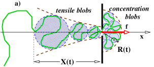
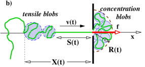
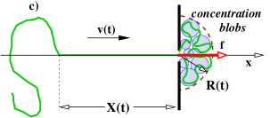
Figure 1: Dynamical response of the polymer chain to the driving force $f$ acting in the pore. Concentration blobs on the trans side make up a “mushroom cap”. Blob sizes on the cis - side are $x$-dependent and have the cylindrical symmetry, while the concentration blobs have a hemispherical symmetry. The front propagation on the cis- and trans- sides are denoted by $X(t)$ and $R(t)$ respectively. (a) For small forces, $T/aN^{\nu}\ll f\leq T/a$, tensile blobs on the cis - side are shaped in the form of a “trumpet” ; (b) For the intermediate forces, $T/a<f\ll(T/a)N^{\nu}$, the part of the chain affected by tension has a “stem-flower” configuration, with the stem length $S(t)$; (c) Finally, for large forces, $f>(T/a)N^{\nu}$, the part of chain affected by tension looks like a “stem”.

II.1.1 Weak forces: $T/aN^{\nu}\ll f\leq T/a$

The tensile blob size $\xi(x,t)$ , located at distance $x$ from the membrane, can be expressed in terms of the corresponding tensile force $f(x,t)$ as follows

$$\xi(x,t)=\dfrac{T}{f(x,t)}.$$ (1)

On the other hand, the local tensile force $f(x,t)$ is balanced by the Stokes friction force acting on the segments located between $x$ and $-X(t)$ (recall that the origin of coordinates, $x=0$, is placed in the pore ), i.e.

$$f(x,t)=6\pi\>\zeta_{0}\int\limits_{-X(t)}^{x}v(x^{\prime},t)\left[\dfrac{\xi(x^{\prime},t)}{a}\right]^{z-2}\>\dfrac{dx^{\prime}}{\xi(x^{\prime},t)}.$$ (2)

In Eq. (2) $dx^{\prime}/\xi(x^{\prime},t)$ counts the number of blobs in the interval $x^{\prime},x^{\prime}+dx^{\prime}$, whereas $\zeta_{0}v(x^{\prime},t)[\xi(x^{\prime},t)/a]^{z-2}$ is the local Stokes friction force, with $\zeta_{0}$ being the friction coefficient DeGennes . The dynamic exponent is equal either $z=2+1/\nu$ or $z=3$ for Rouse or Zimm dynamics respectively. We also keep explicitly the coefficient $6\pi$ bearing in mind that in both, Rouse or Zimm, cases we have a succession of spherical units, beads or impenetrable blobs, which are responsible for Stokes friction.

In order to simplify the mathematical treatment of the tensile propagation (on the cis - side) and the crowding effect on the trans side as well as to gain more physical insight into the process we will rely on the “homogeneous approximation”. In this case the tensile propagation consideration is based on the “two phase picture” Sakaue_1 ; Sakaue_2 where the moving and quiescent domains are separated by a narrow tension front. Moreover, the moving domain is treated as a uniform block within which all monomers are moving with the same time-dependent representative velocity $v(t)$. In this case instead of Eq. (2) we have

$$f(x,t)=6\pi\>\zeta_{0}\>v(t)\int\limits_{-X(t)}^{x}\left[\dfrac{\xi(x^{\prime},t)}{a}\right]^{z-2}\>\dfrac{dx^{\prime}}{\xi(x^{\prime},t)}.$$ (3)

By making use the local relationships $\xi(x,t)=T/f(x,t)$ we have

$$\dfrac{1}{\xi(x,t)}=\dfrac{6\pi\>\zeta_{0}}{T}\>v(t)\int\limits_{-X(t)}^{x}\left[\dfrac{\xi(x^{\prime},t)}{a}\right]^{z-2}\>\dfrac{dx^{\prime}}{\xi(x^{\prime},t)},$$ (4)

which when recast in differential form reads

$$\dfrac{d\xi}{dx}=-\dfrac{6\pi\>\zeta_{0}\>v(t)}{Ta^{z-2}}\>\xi^{z-1}.$$ (5)

Equation 5 should be supplemented with the boundary condition

$$\xi(x=0,t)=\dfrac{T}{F(t)},$$ (6)

where $F(t)$ stands for the resulting force in the pore (see below for more details). As a result the solution reads

$$\xi(x,t)=\dfrac{a}{\left\{\dfrac{6\pi\>\zeta_{0}v(t)}{T}\>x+\left[\dfrac{aF(t)}{T}\right]^{z-2}\right\}^{1/(z-2)}}$$ (7)

The second condition at the free boundary, i.e. at $x=-X(t)$, claims that the tension $f(x=-X(t),t)=T/\xi(x=-X(t),t)=0$. Taking into account Eq. (7) we have $-6\pi\>\zeta_{0}v(t)X(t)/T+[aF(t)/T]^{z-2}=0$ and hence the chain velocity obeys

$${\widetilde{v}}(t)=\dfrac{[{\widetilde{F}}(t)]^{z-2}}{{\widetilde{X}}(t)},$$ (8)

where we introduced the dimensionless quantities: ${\widetilde{v}}(t)\equiv 6\pi\>\zeta_{0}av(t)/T$, ${\widetilde{F}}(t)\equiv aF(t)/T$ and ${\widetilde{X}}(t)\equiv X(t)/a$. Taking Eq. (8) into account Eq. (7) could be represented in the form

$${\widetilde{\xi}}({\widetilde{x}},t)=\dfrac{1}{\{{\widetilde{v}}(t)[{\widetilde{x}}+{\widetilde{X}}(t)]\}^{1/(z-2)}},$$ (9)

where the notations ${\widetilde{x}}\equiv x/a$ and ${\widetilde{\xi}}\equiv\xi/a$ have been used.

Using the global material balance of monomers we arrive at the following relation

$$\int\limits_{-X(t)}^{0}\>\left[\dfrac{\xi(x,t)}{a}\right]^{1/\nu}\dfrac{dx}{\xi(x,t)}+M(t)=N(t),$$ (10)

where the first integral counts the number of monomers in the moving domain (see Fig. 1), $M(t)$ denotes the number of translocated monomers and $N(t)$ stands for the total number of monomers subjected to tension during the time interval $[0,t]$. At time $t=0$ all these $N(t)$ monomers were in equilibrium and occupying a region of size $X(t)$. In other words $N(t)$ and $X(t)$ are related by the Flory expression, i.e.

$$X(t)=a[N(t)]^{\nu}.$$ (11)

Substituting Eq. (9) and Eq. (11) in Eq. (10) for the material balance, leads to

$$\dfrac{{\widetilde{X}}(t)}{C_{1}\>[{\widetilde{F}}(t)]^{\frac{1}{\nu}-1}}+M(t)=[{\widetilde{X}}(t)]^{\frac{1}{\nu}},$$ (12)

where the numerical coefficient $C_{1}=1-(1-\nu)/[\nu(z-2)]$, i.e. $C_{1}=\nu$ for Rouse and $C_{1}=2-1/\nu$ for Zimm models.

The flux of monomers at the pore $j_{0}(t)=\rho(x=0,t)v(t)$ (where $\rho(x,t)=[\xi(x,t)/a]^{1/\nu}/\xi(x,t))$ is the linear density of monomers) should be taken equal to $dM(t)/dt$ , i.e. as a result

$$\dfrac{dM(t)}{dt}=\left[\dfrac{\xi(x=0,t)}{a}\right]^{1/\nu}\dfrac{v(t)}{\xi(x=0,t)},$$

or in terms of the dimensionless variables

$$\dfrac{dM(t)}{d{\widetilde{t}}}=\dfrac{[{\widetilde{F}}(t)]^{z-1-1/\nu}}{6\pi\>{\widetilde{X}}(t)}.$$ (13)

where we have used Eq. (8) and Eq. (9) and also introduced the dimensionless time ${\widetilde{t}}=t/\tau_{0}$, with $\tau_{0}=a^{2}\zeta_{0}/T$.

It is worth mentioning that the foregoing consideration refers to the tension propagation. After the characteristic time $\tau_{1}$ when the tension has propagated to the last monomer of the chian, i.e. at ${\widetilde{X}}(\tau_{1})=N^{\nu}$ or $N(\tau_{1})=N$, the second, so-called tail retraction, stage sets in. For $t>\tau_{1}$ the material balance equation (12) should therefore be replaced by the following relation

$$\dfrac{{\widetilde{X}}(t)}{C_{1}\>[{\widetilde{F}}(t)]^{\frac{1}{\nu}-1}}+M(t)=N.$$ (14)

In the case of intermediate driving forces, i.e. for $(T/a)<f\ll T/a$, the foregoing equations Eqs. (8), (12), (13), (14), will change form, which we will discuss next.

II.1.2 Intermediate forces: $T/a<f\ll(T/a)N^{\nu}$

In this case the translocation starts with a “stem” formation and the velocity decreases , so that at the moment $t=\tau^{\sharp}$ the drag force at the stem-flower junction point becomes $T/a$, i.e. $6\pi\zeta_{0}v(\tau^{\sharp})=T/a$ or in dimensionless notations ${\widetilde{v}}(\tau^{\sharp})=1$. At $t>\tau^{\sharp}$ the “stem-flower” regime sets in (see Fig. 1b) with the “flower” part following the same as for the weak force differential equation, Eq. (5). However, the boundary condition is different and reads $\xi(x=-S(t))=a$. Thus, the “flower” part follows the law

$$\xi({\widetilde{x}},t)=\dfrac{a}{\left\{1+{\widetilde{v}}(t)[{\widetilde{x}}+{\widetilde{S}}(t)]\right\}^{1/(z-2)}},$$ (15)

where the dimensionless values ${\widetilde{x}}=x/a$ and ${\widetilde{S}}(t)=S(t)/a$. Again at ${\widetilde{x}}=-{\widetilde{X}}(t)$ the tensile force is zero, i.e. $f({\widetilde{x}}=-{\widetilde{X}}(t))=T/\xi({\widetilde{x}}=-{\widetilde{X}}(t),t)=0$ and by making use Eq. (15) we have

$${\widetilde{X}}(t)={\widetilde{S}}(t)+\dfrac{1}{{\widetilde{v}}(t)}.$$ (16)

The material balance is in this case given by (cf. Eq. (10))

$$\int\limits_{-{\widetilde{X}}(t)}^{-{\widetilde{S}}(t)}\>\left[\dfrac{\xi({\widetilde{x}},t)}{a}\right]^{1/\nu}\dfrac{a\>d{\widetilde{x}}}{\xi({\widetilde{x}},t)}+{\widetilde{S}}(t)+M(t)=N(t),$$ (17)

which after using Eqs. (11) and (15) takes the form

$$\dfrac{1}{C_{1}{\widetilde{v}}(t)}+{\widetilde{S}}(t)+M(t)=[{\widetilde{X}}(t)]^{1/\nu}.$$ (18)

To exclude ${\widetilde{v}}(t)$ and ${\widetilde{S}}(t)$ we write down the force balance for the stem, i.e. $6\pi\zeta_{0}v(t){S}(t)/a=F(t)-T/a$ or in terms of dimensionless variables ${\widetilde{v}}(t){\widetilde{S}}(t)={\widetilde{F}}(t)-1$. Combination of this result with Eq. (16) leads to

$${\widetilde{v}}(t)=\dfrac{{\widetilde{F}}(t)}{{\widetilde{X}}(t)},$$ (19)

and

$${\widetilde{S}}(t)={\widetilde{X}}(t)-\dfrac{{\widetilde{X}}(t)}{{\widetilde{F}}(t)}.$$ (20)

Thus, the material balance Eq. (18) becomes

$$\left(\dfrac{1}{C_{1}}-1\right)\dfrac{{\widetilde{X}}(t)}{{\widetilde{F}}(t)}+{\widetilde{X}}(t)+M(t)=\left[{\widetilde{X}}(t)\right]^{1/\nu}$$ (21)

For the same reason as in the weak force case Eq. (21) only applies for $t~{}\leq~{}\tau_{1}$. For $t>\tau_{1}$ Eq. (21) should be must be replaced by the expression

$$\left(\dfrac{1}{C_{1}}-1\right)\dfrac{{\widetilde{X}}(t)}{{\widetilde{F}}(t)}+{\widetilde{X}}(t)+M(t)=N.$$ (22)

The flux of monomers through the pore is $dM(t)/dt=v(t)/a$ or in fully dimensionless variables this reads

$$\dfrac{dM({\widetilde{t}})}{d{\widetilde{t}}}=\dfrac{{\widetilde{F}}({\widetilde{t}})}{6\pi{\widetilde{X}}({\widetilde{t}})},$$ (23)

where we have invoked Eq. (19). We next turn to the strongly forced chain.

II.1.3 Strong forces: $f>(T/a)N^{\nu}$

In this case the moving domain on the cis-side is completely stretched (“stem”) as shown in Fig. 1c and the force balance reads

$${\widetilde{F}}(t)={\widetilde{v}}(t){\widetilde{X}}(t).$$ (24)

The material balance for $t<\tau_{1}$ is simply given by

$${\widetilde{X}}(t)+M(t)=N(t).$$ (25)

Taking into account again that $N(t)^{\nu}={\widetilde{X}}(t)$ we have

$${\widetilde{X}}(t)+M(t)=[{\widetilde{X}}(t)]^{1/\nu}.$$ (26)

For $t>\tau_{1}$ the material balance takes the form

$${\widetilde{X}}(t)+M(t)=N.$$ (27)

where $N$ is the chain length.

Equation for $M(t)$ has the following form (in dimensionless variables) $dM(t)/d{\widetilde{t}}={\widetilde{v}}(t)/6\pi$. Taking into account the force balance equation, Eq. (24) we arrive at

$$\dfrac{dM(t)}{d{\widetilde{t}}}=\dfrac{{\widetilde{F}}(t)}{6\pi{\widetilde{X}}(t)},$$ (28)

which is exactly equivalent to the corresponding Eq. (23) for the “stem-flower” case. It is also interesting that this equation exactly corresponds to Eq. (13) taken for the Rouse model, i.e. at $z-2=1/\nu$.

The two equations, Eq. (12) (or the corresponding Eq. (14)) and Eq. (13), for two unknowns, ${\widetilde{X}}(t)$ and $M(t)$, are still not closed, because the resulting force ${\widetilde{F}}(t)$ acting in the pore is not simply a given function of time. This force includes the driving force $f$ which is balanced by the pore friction as well as the osmotic pressure on the trans- side (crowding effect). In order to quantify the last one we should investigate the blob dynamics on the trans-side in more detail, to which we turn in the next subsection.

II.2 Concentration-blob picture on the trans-side

In the “homogeneous approximation” used before, the monomer density in the hemisphere of size $R(t)$ is uniform and mass density $\phi(t)=a^{3}M(t)/[R(t)]^{3}$. The concentration blob size $\xi(t)$ is now given by

$$\xi(t) =a[\phi(t)]^{\nu/(1-3\nu)}=a[{\widetilde{R}}(t)^{3}/M(t)]^{\nu/(3\nu-1)},$$ (29)

where the dimensionless ${\widetilde{R}}(t)\equiv R(t)/a$ was introduced. This approximation in the context of polymer decompression dynamics has been previously discussed by Sakaue et al. Sakaue_4 .

We next derive the differential equation for ${\widetilde{R}}(t)$. The confinement free energy $\Delta{\cal F}$ can be written as a number of concentration blobs, $R(t)^{3}/\xi(t)^{3}$, times the temperature $T$ Sakaue_4 ; DeGennes . If we next use Eq. (29) we find

$$\Delta{\cal F}=T\dfrac{R(t)^{3}}{\xi(t)^{3}}=T\>C_{2}\>\left[\dfrac{M(t)^{\nu}}{{\widetilde{R}}(t)}\right]^{3/(3\nu-1)},$$ (30)

where $C_{2}$ is a constant of order unity. The equation of motion for ${\widetilde{R}}(t)$ can be obtained by equating the friction (or drag) force $f_{\rm fr}$ to the thermodynamic force $f_{\rm th}=-\partial\Delta{\cal F}/\partial R$. In the Rouse model the chain is fully free-draining and all beads experience the same friction, i.e. $f_{\rm fr}=6\pi\zeta_{0}M(t)dR(t)/dt$, where $\zeta_{0}$ is a monomer friction coefficient. In the Zimm model the friction force is defined by the geometric dimension of the trans-domain times the velocity, i.e. $f_{\rm fr}=6\pi\eta_{0}R(t)dR(t)/dt$, where $\eta_{0}\sim\zeta_{0}/a$ is the solvent viscosity. The thermodynamic force $f_{\rm th}$ is given by

$$f_{\rm th}=-\dfrac{\partial}{\partial R}\>\Delta{\cal F}\simeq T\left(\dfrac{3C_{2}}{3\nu-1}\right)\dfrac{[M]^{3\nu/(3\nu-1)}}{a[{\widetilde{R}}]^{(3\nu+2)/(3\nu-1)}}$$ (31)

Balancing the friction and thermodynamic forces, $f_{\rm fr}=f_{\rm th}$, we find the governing equation for $\widetilde{R}$ in the Rouse and Zimm case as

$$\dfrac{d{\widetilde{R}}}{d{\widetilde{t}}}=\begin{cases}\dfrac{C_{2}[M]^{1/(3\nu-1)}}{2\pi(3\nu-1){\widetilde{R}}^{(3\nu+2)/(3\nu-1)}},&\mbox{Rouse}\\ \\ \dfrac{C_{2}[M]^{3\nu/(3\nu-1)}}{2\pi(3\nu-1){\widetilde{R}}^{(6\nu+1)/(3\nu-1)}},&\mbox{Zimm}\end{cases}$$ (32)

Equation (32) is usually referred to as the Onsager equation Puri . Finally, we discuss the resulting force $F(t)$ acting in the pore.

II.3 Resulting force $F(t)$ in the pore

The driving force $f$ push the monomers in the trans-domain which has a hemispherical form of size $R(t)$. In the “homogeneous approximation” this process could be seen as the work done against the osmotic pressure within the hemisphere, i.e. the monomer in the pore which is about to translocate could be thought of as a small piston. In other words, the driving force is counterbalanced by the osmotic pressure times the pore cross-area. Thus, the resulting force $F(t)$ in the pore is made up of following components: the external driving force $f$ which is mitigated by the counterbalance force $f_{\rm count}(t)$, caused by the osmotic pressure in the compressed trans-domain (crowding effect), as well as by the the friction force $f_{\rm pore}(t)$ in the pore, i.e.

$$F(t)=f-f_{\rm count}(t)-f_{\rm pore}(t).$$ (33)

The force $f_{\rm count}(t)$ is defined as the osmotic pressure times the cross-sectional area of the pore, i.e.

$$f_{\rm count}(t)=\underbrace{\left(-\dfrac{\partial\Delta{\cal F}}{\partial V}\right)}_{\rm osmotic\>\>pressure}\times\underbrace{\dfrac{\pi}{4}a^{2}}_{\rm area}=\dfrac{T}{a}\left[\dfrac{3C_{2}}{8(3\nu-1)}\right]\left(\dfrac{M}{{\widetilde{R}}^{3}}\right)^{3\nu/(3\nu-1)},$$

where we took into account that the the trans-domain (see Fig. 1) has the volume $V=(2\pi/3)R(t)^{3}$. In the dimensionless notations

$${\widetilde{f}}_{\rm count}(t)=\left[\dfrac{3C_{2}}{8(3\nu-1)}\right]\left(\dfrac{M(t)}{{\widetilde{R}}(t)^{3}}\right)^{3\nu/(3\nu-1)}.$$ (34)

The pore friction force (in the dimensionless units) ${\widetilde{f}}_{\rm pore}(t)\equiv af_{\rm pore}/T=6\pi\zeta_{p}av(t)/T=(\zeta_{p}/\zeta_{0}){\widetilde{v}}(t)$, where $\zeta_{p}$ is the pore friction coefficient and we have used the notation ${\widetilde{v}}(t)\equiv 6\pi\zeta_{0}av(t)/T$. Taking into account Eq. (8) we have

$${\widetilde{f}}_{\rm pore}(t)=\dfrac{\zeta_{p}[{\widetilde{F}}(t)]^{z-2}}{\zeta_{0}{\widetilde{X}}(t)}.$$ (35)

Finally, by using Eq. (33) we obtain the algebraic equation

$${\widetilde{F}}(t)={\widetilde{f}}-\left[\dfrac{3C_{2}}{8(3\nu-1)}\right]\left[\dfrac{M(t)}{{\widetilde{R}}(t)^{3}}\right]^{3\nu/(3\nu-1)}-\dfrac{\zeta_{p}[{\widetilde{F}}(t)]^{z-2}}{\zeta_{0}{\widetilde{X}}(t)}.$$ (36)

For intermediate and strong forces (which corresponds to “stem-flower” and “stem” scenario, respectively) the pore friction reads ${\widetilde{f}}_{\rm pore}(t)=(\zeta_{p}/\zeta_{0}){\widetilde{v}}(t)=(\zeta_{p}/\zeta_{0}){\widetilde{F}}(t)/{\widetilde{X}}(t)$, where we have used Eq. (19) (or analogously Eq. (24) for the “stem” case). As a result, Eq. (36) will be replaced by

$${\widetilde{F}}(t)={\widetilde{f}}-\left[\dfrac{3C_{2}}{8(3\nu-1)}\right]\left[\dfrac{M(t)}{{\widetilde{R}}(t)^{3}}\right]^{3\nu/(3\nu-1)}-\dfrac{\zeta_{p}[{\widetilde{F}}(t)]}{\zeta_{0}{\widetilde{X}}(t)},$$ (37)

or, equivalently,

$${\widetilde{F}}(t)=\dfrac{{\widetilde{f}}-\left[\dfrac{3C_{2}}{8(3\nu-1)}\right]\left[\dfrac{M(t)}{{\widetilde{R}}(t)^{3}}\right]^{3\nu/(3\nu-1)}}{1+\dfrac{\zeta_{p}}{\zeta_{0}{\widetilde{X}}(t)}}.$$ (38)

As a result we have four equations, i.e. Eqs. (12) , (13), (32) and (36) (in the case of intermediate forces these equations are Eqs. (21), (23), (32) and (38)) for four unknowns ${\widetilde{X}}(t)$, ${\widetilde{R}}(t)$, $M(t)$ and ${\widetilde{F}}(t)$. The translocation problem within this model is treated self-consistently, which means that the resulting force in the pore $F(t)$ is not given but depends on the front positions on cis, ${\widetilde{X}}(t)$, and trans, ${\widetilde{R}}(t)$, sides as well as on the number of translocated monomers $M(t)$. In the next section we discuss the numerical solution of this set of equations. In doing so, we will compare the results with the simplified case without crowding and pore friction Dubbeldam . A more detailed exposition for this case is given in Appendix A.

III Numerical computations

The resulting four equations, Eqs. (12) , (13), (32) and (36), for the four variables: ${\widetilde{X}}(t)$, ${\widetilde{R}}(t)$, $M(t)$ and ${\widetilde{F}}(t)$ are known as the semi-explicit differential-algebraic equations (DAE) Brenan . For these particular DAE we can distinguish between the differential variables: ${\widetilde{R}}(t)$ and $M(t)$, and the algebraic ones: ${\widetilde{X}}(t)$ and ${\widetilde{F}}(t)$. In the case of intermediate forces, i.e. $1<{\widetilde{f}}<N^{\nu}$, the corresponding equations are Eqs. (21), (23), (32) and (38). By fixing the initial conditions for the differential variables, ${\widetilde{R}}(0)$ and $M(0)$, the corresponding initial values for ${\widetilde{X}}(0)$ and ${\widetilde{F}}(0)$ are obtained from Eqs.(12), (36) employing the Newton-Ralphson method. By alternatingly solving the differential equations for ${\widetilde{R}}$ and $M$ (using the Euler forward method), and the algebraic equations for ${\widetilde{X}}(t)$ and ${\widetilde{F}}(t)$, we obtain the solution of the system of DAE. In all calculations the constant $C_{2}$, which naturally appears in the scaling expression for the free energy Eq. (30), has been set to $C_{2}=1$. However, we verified that the numerical results do not change notably even when $C_{2}$ was set to $10$.

In Fig. 2, we show the translocation time $\tau$ vs. chain length $N$ or two different driving forces $\widetilde{f}=1$ and $\widetilde{f}=10$. We find scaling $\tau\propto N^{\alpha}$ in a wide range of chain lengths, $10^{2}<N<10^{6}$. We note that for ${\widetilde{f}}=1$ and ${\widetilde{f}}=10$ we have used for calculations the “trumpet” and “stem-flower” scenarios, respectively. The corresponding results are shown in Fig. 2. First of all one can see that trans side crowding practically does not affect the scaling behavior: the curve corresponding to the case without crowding and pore friction (shown by red filled circles in Fig.  2) coincides with the case with crowding but vanishing pore friction, i.e. $r=\xi_{p}/\xi_{0}=0$ (shown by blue boxes in Fig.  2). In other words the impact of the “crowding effect” by itself is almost negligible. Only for larger pore friction ratios, $r=10$ and $r=100$, the exponent $\alpha$ mildly changes (especially for a relatively small force, ${\widetilde{f}}=1$, shown in Fig. 2a); larger values of $r$ correspond to smaller values of $\alpha$. For the stronger force, ${\widetilde{f}}=10$, the value of the translocation exponent falls to $\alpha=1.12$ for the high friction pore, $r=\xi_{p}/\xi_{0}=100$ (cf. Fig.2b ). This value is smaller than the value of $\alpha$ for the no crowding case, $\alpha=1+\nu=1.588$ (shown by filled red circles in Fig. 2b ), and close to the linear scaling law, $\tau\propto N$, found experimentally by Kasianowicz et al. Kasianowicz for polyuridylic acid in the range of 100 - 500 nucleotides. On the other hand, experiments on double-stranded DNA translocation through a solid-state nanopore lead to the exponent $\alpha=1.27$ Storm ; Storm_1 , which is close to our findings for ${\widetilde{f}}=10$ and $10<r<100$ shown in Fig.2b.

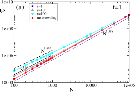
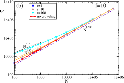
Figure 2: Translocation time $\tau$ dependence on $N$ (with crowding and pore friction effects) for different values of the forces: (a) ${\widetilde{f}}=1$ and (b) ${\widetilde{f}}=10$. The different pore frictions ratios, $r=\xi_{p}/\xi_{0}$, are specified in the legend. The scaling for the no crowding and no pore friction case (outlined in Appendix A) is shown for reference by filled red round symbols.

Another interesting behavior exhibited by Fig. 2 is the finite chain length effect due to the pore friction. One can see that as the chain length $N$ increases the scaling exponent $\alpha$ approaches the “no crowding and no pore friction” case, i.e. $\alpha=1+\nu$ (see Appendix A). Moreover, the larger the pore friction, the greater is the chain length crossover $N_{c}$. For example, for ${\widetilde{f}}=10$ and $r=100$ the crossover chain length $N_{c}\approx 10^{5}$. This behavior is in full agreement with results of Ikonen et al. Ikonen ; Ikonen_2 .

Next we investigate the dynamics of the translocation process. Figure 3 shows the number of translocated monomers $M(t)$ and the resulting force ${\widetilde{F}}(t)$ as functions of time. As one can see from Fig. 3a the translocation velocity initially slightly decreases, however, when the chain has nearly threaded the pore it experiences a large acceleration as witnessed by the almost vertical tangent to the curve when $M(t)$ approaches the chain length $N=400$. In Fig. 3a we compare in a clear way the simplified model without crowding and pore friction (as discussed in Appendix A), on the one hand, and the model with crowding but without pore friction friction ($r=0$), on the other hand. This comparison shows once more that crowding by itself hardly influences the speed of the translocation process. Alternatively, a large pore friction coefficient (as compared with the bulk friction coefficient) leads to a clear dynamical slowing down.

The resulting force evolution given in Fig. 3b first shows a gradual increase which after reaching its maximum value rapidly decreases to zero. It is interesting that the maximum of force is attained when the propagating front on the cis - side has reached the end of the polymer chain (tension propagation stage). After that the whole chain, which participates in the translocation process, starts to accelerate. During this stage (known as the tail retraction stage Ikonen_1 ; Ikonen_2 ) the tensile force in the chain starts to drop and vanishes when the chain has fully translocated through the pore.

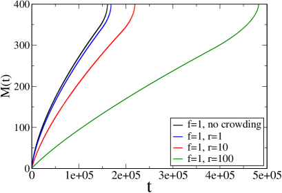
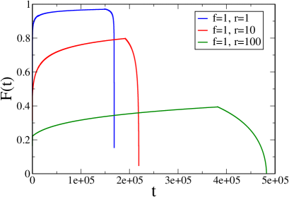
Figure 3: In (a) the number of translocated monomers for a N=400 chain is shown as function of time. The upper curve corresponds to the sipmified “no crowding and no pore friction case” outlined in Appendix A. (b) the dependence of the resulting force in the pore as a function of time is displayed.

The same two stages of translocation also could be seen on the waiting time distribution $w(M)$ which is defined as the time that takes for the transition $M\rightarrow M+\Delta M$ (cf. ref. Linna_3 ; Ikonen_1 ; Ikonen_2 ). It is apparent that in the continuous limit the waiting time distribution is nothing but the inverse translocation coordinate velocity, i.e. $w(M)=(dM/dt)^{-1}$. In Figure 4 we show these distributions for different chain lengths, pore frictions and forces. Again one can discern the tensile force propagation stage during which transloaction slows down, which is then followed by the chain tail retraction stage during which the translocation process speeds up. Our results are in qualitative agreemenent with the findings based on MD-simulation and BDTP-model Linna_3 ; Ikonen_1 ; Ikonen_2 ).

Figure 4: Waiting time distribution function, $w(M)=(dM/dt)^{-1}$, as a function of $M$ for different forces: a) $f=1$ and b) $f=10$. Chain lengths, $N=100,400,1000$, and friction coefficients ratios, $r=\xi_{p}/\xi_{0}=1,10$, are shown in legends.

IV Conclusions

We have given a detailed theoretical interpretation of crowding and pore friction effects in the course of driven polymer translocation. Translocation dynamics is treated self-consistently when the resulting force in the pore, $F(t)$, depends on the front positions on cis, $\widetilde{X}(t)$, and trans, $\widetilde{R}(t)$, sides as well as on the number of translocated monomers $M(t)$. This approach provides a generalization of the BDTP-model Ikonen ; Ikonen_1 ; Ikonen_2 where the time-dependent friction coefficient of the cis side moving domain was taken from the simplified model without crowding and pore friction. The resulting four differential - algebraic equations for four dynamical variables, ${\widetilde{X}}(t)$, ${\widetilde{R}}(t)$, $M(t)$ and ${\widetilde{F}}(t)$, were derived by taking into account the tensile force propagation on the cis - side of the membrane as well as the concentration blob picture on the trans-side. Our detailed numerical solutions of these equations show that the translocation dynamics is scarcely affected by the crowding itself, which is consistent with previous findings Ikonen_1 ; Ikonen_2 . On the other hand, in the presence of pore friction the translocation process not only becomes slower but also the translocation exponent $\alpha$ (especially for relatively large driving forces) decreases as compared to the idealized case without crowding and pore friction, i.e. $\alpha<1+\nu$. With increase of chain length the translocation scaling asymptotically approaches the “no crowding no pore friction” case, i.e. the scaling exponent $\alpha=1+\nu$ (see Appendix A). The crossover is very broad with the corresponding critical chain length $N_{c}\approx 10^{5}$ (for large force and high pore friction). This conclusion is in a full agreement with results of Ikonen et al. Ikonen ; Ikonen_2 . Hence the translocation exponent $\alpha$ is not universal and (for relatively short polymer chains and strong forces) mainly the pore friction could lower its value. This, in turn, explains the large variety of $\alpha$ values which have been reported in experiments Kasianowicz ; Storm ; Storm_1 and computer simulations Milchev .

Appendix A Simplification: no crowding and no pore friction

Let’s now simplify matters by neglecting crowding and pore friction effects. In this case the effective force ${\widetilde{F}}(t)={\widetilde{f}}$ and we go back to the case which was investigated in ref. Dubbeldam . Then Eqs. (13) and (12) become closed and we have

$$\dfrac{dM(t)}{d{\widetilde{t}}}=\dfrac{{\widetilde{f}}^{z-1-1/\nu}}{6\pi\>{\widetilde{X}}(t)}$$ (39)

and

$$\dfrac{{\widetilde{X}}(t)}{C_{1}\>{\widetilde{f}}^{\frac{1}{\nu}-1}}+M(t)=[{\widetilde{X}}(t)]^{\frac{1}{\nu}}$$ (40)

At $t>\tau_{1}$ instead of the material balance equation Eq. (40) we have

$$\dfrac{{\widetilde{X}}(t)}{C_{1}\>{\widetilde{f}}^{\frac{1}{\nu}-1}}+M(t)=N$$ (41)

This simplified case enables to solve the problem analytically. Really, after differentiation of Eq. (40) and combination with Eq. (39) we have

$$\dfrac{1}{\nu}\left[1-({\widetilde{f}}{\widetilde{X}})^{1/\nu-1}\right]\>\dfrac{d{\widetilde{X}}}{d\>{\widetilde{t}}}=-\dfrac{{\widetilde{f}}^{z-2}}{6\pi{\widetilde{X}}}$$ (42)

where we have also used that for the Rouse model $C_{1}=\nu$. This equation could be easily solved with the natural initial condition ${\widetilde{X}}(0)=1/{\widetilde{f}}$. The corresponding solution reads

$${\widetilde{t}}=t_{0}+\dfrac{6\pi}{1+\nu}\;{\widetilde{f}}^{1/\nu-z+1}{\widetilde{X}}^{1/\nu+1}\left[1-\dfrac{1+\nu}{\nu({\widetilde{f}}{\widetilde{X}})^{1/\nu-1}}\right]$$ (43)

where $\tau_{0}=6\pi/[\nu(1+\nu){\widetilde{f}}^{z}]$. The first stage of the translocation process, tension propagation, is continued up to $t=\tau_{1}$ when the tension attain the very last monomer, i.e. ${\widetilde{X}}(\tau_{1})=N^{\nu}$. In this case the characteristic (dimensionless) time of the first stage reads

$$\tau_{1}=\dfrac{6\pi}{1+\nu}\;{\widetilde{f}}^{1/\nu-z+1}N^{1+\nu}\left[1-\dfrac{1+\nu}{\nu({\widetilde{f}}N^{\nu})^{1/\nu-1}}\right]$$ (44)

At the second stage, tail retraction, the material balance equation is given by Eq. (41), which, due to Eq. (39), yields

$${\widetilde{X}}\>\dfrac{d{\widetilde{X}}}{d{\widetilde{t}}}=-\dfrac{\nu}{6\pi}\>{\widetilde{f}}^{z-2}$$ (45)

As it can be seen at the tail retraction regime $d{\widetilde{X}}/d{\widetilde{t}}<0$ and ${\widetilde{X}}$ decreases from ${\widetilde{X}}(\tau_{1})=N^{\nu}$ up to ${\widetilde{X}}(\tau_{\rm fin})=0$, where $\tau_{\rm fin}$ is the final time moment of the translocation. The solution of Eq. (45) has the form

$${\widetilde{t}}=\tau_{\rm fin}-\dfrac{3\pi{\widetilde{X}}^{2}}{\nu{\widetilde{f}}^{z-2}}$$ (46)

The second stage of translocation lasts $\tau_{2}=\tau_{\rm fin}-\tau_{1}$ and due to Eq. (46) we have

$$\tau_{2}\propto\dfrac{N^{2\nu}}{{\widetilde{f}}^{z-2}}$$ (47)

As a result the total traslocation time is given as Dubbeldam

$$\langle\tau\rangle = \tau_{1}+\tau_{2}$$ (48)

$$= B_{1}\dfrac{N^{1+\nu}}{{\widetilde{f}}^{z-1-1/\nu}}+B_{2}\dfrac{N^{2\nu}}{{\widetilde{f}}^{z-2}}$$

For the Rouse case (i.e. when $z=2+1/\nu$) we arrive at the result

$$\langle\tau\rangle=B_{1}\dfrac{N^{1+\nu}}{{\widetilde{f}}}+B_{2}\dfrac{N^{2\nu}}{{\widetilde{f}}^{1/\nu}}$$ (49)

This important result, which indicates the crossover between the tension propagation and tail retraction regimes as the chain length $N$ increases, has been derived for the first time in ref. Dubbeldam (see Eq. (2.26) in this reference) by a slightly different method. Eq. (49) predicts that the effective translocation exponent falls in the range $2\nu\leqslant\alpha\leqslant 1+\nu$, which closely agrees with MD-findings by Luo et al. Luo . This crossover could also lead, along with polymer-pore friction, to lower values of the translocation exponent $\alpha$ for relatively small chain lengths.

Lastly, we should mention that the result given by Eq. (49) leads to the correct scaling for the unbiased translocation case when the driving force ${\widetilde{f}}$ is vanishingly small. Really, in this case ${\widetilde{f}}\longrightarrow 1/N^{\nu}$ (this is the lower bound for the Pincus blob formation DeGennes ) and Eq. (49) can be written as $\langle\tau\rangle\propto N^{2\nu+1}$. This result was obtained first by Kantor&Kardar Kantor in a different way.

References

- (1) M. Muthukumar, Polymer Translocation, CRC Press, Taylor& Francis Group, London, NY, 2011.
- (2) T. Sakaue, Phys. Rev. E 81, 041808 (2010).
- (3) T. Saito, T. Sakaue, Eur. Phys. J. E 34, 135 (2011).
- (4) T. Saito, T. Sakaue, arXiv: 1205.3861v.3 (2012).
- (5) J. L. A. Dubbeldam, V.G. Rostiashvili, A. Milchev, T.A. Vilgis, Phys. Rev. E 85, 041801 (2012).
- (6) P. Rowghanian, A.Y. Grosberg, J. Phys. Chem. B 115, 141127 (2011).
- (7) V.V. Lehtola, R. P. Linna, K. Kaski, Europhys. Lett. 85, 58006 (2009).
- (8) V.V. Lehtola, K. Kaski, R. P. Linna, Phys. Rev. E, 031908 (2010).
- (9) A. Bhattacharya, K. Binder, Phys. Rev. E 81, 041804 (2010).
- (10) T. Sakaue, N. Yoshinaga, Phys. Rev. Lett. 102, 148302 (2009).
- (11) P. G. de Gennes, Scaling Concept in Polymer Physics, Cornell University Press, Ithaca, NY, 1979.
- (12) T. Saito, T. Sakaue, Phys. Rev. E 88, 042606 (2013).
- (13) P.M. Suhonen, K. Kaski, R. P. Linna, submitted (http://arxiv.org/abs/1405.0902) (2014).
- (14) T. Ikonen, A. Bhattacharya, T. Ala-Nissila, W. Sung, Europhys. Lett. 103, 38001 (2013).
- (15) T. Ikonen, A. Bhattacharya, T. Ala-Nissila, W. Sung, Phys. Rev. E 85, 051803 (2012).
- (16) T. Ikonen, A. Bhattacharya, T. Ala-Nissila, W. Sung, J. Chem. Phys. 137, 085101 (2012).
- (17) A. Bhattacharya, Phys. Proc. 3, 1411 (2010).
- (18) C.M. Edmonds, Y.C. Hudiono, A.G. Ahmadi, P.J. Hesketh, J.Chem. Phys. 136, 065105 (2012).
- (19) J. Chuang, Y. Kantor, M. Kardar, Phys. Rev. E 65, 011802 (2001).
- (20) S. Dattagupta, S. Puri, Dissipative Phenomena in Condensed Matter, Springer-Verlag, Berlin, 2004.
- (21) K.E. Brenan, S.L. Campbell, L.R. Petzold, Numerical Solution of Initial-Value problems in Differential-algebraic Equations, North-Holland, Amsterdam, 1989.
- (22) J. Kasianowicz, E. Brandin, J. Golovchenko, D. Branton, D. Deamer, Proc. Natl. Acad. Sci. USA 93, 13770 (1996).
- (23) A.J. Strom, C. Strom, J.H. Chen, H.W. Zandbergen, J-F. Joanny, C. Dekker, Nano Lett. 5, 1193 (2005).
- (24) A.J. Strom, J. H. Chen, H. W. Zandbergen, C. Dekker, Phys. Rev. E 71, 051903 (2005).
- (25) J.L.A. Dubbeldam, V.G. Rostiashvili, A. Milchev, T.A. Vilgis, Phys. Rev. E 87, 032147 (2013).
- (26) A. Milchev, J. Phys. Cond. Matt. 23, 103101 (2011).
- (27) K. Luo, S.T.T. Ollila, I. Huopaniemi, T. Ala-Nissila, P. Pomorski, M. Kattunen, Phys. Rev. E 78, 050901(R) (2008).