Irreversible Langevin samplers and variance reduction: a large deviations approach
Abstract.
In order to sample from a given target distribution (often of Gibbs type), the Monte Carlo Markov chain method consists in constructing an ergodic Markov process whose invariant measure is the target distribution. By sampling the Markov process one can then compute, approximately, expectations of observables with respect to the target distribution. Often the Markov processes used in practice are time-reversible (i.e., they satisfy detailed balance), but our main goal here is to assess and quantify how the addition of a non-reversible part to the process can be used to improve the sampling properties. We focus on the diffusion setting (overdamped Langevin equations) where the drift consists of a gradient vector field as well as another drift which breaks the reversibility of the process but is chosen to preserve the Gibbs measure. In this paper we use the large deviation rate function for the empirical measure as a tool to analyze the speed of convergence to the invariant measure. We show that the addition of an irreversible drift leads to a larger rate function and it strictly improves the speed of convergence of ergodic average for (generic smooth) observables. We also deduce from this result that the asymptotic variance decreases under the addition of the irreversible drift and we give an explicit characterization of the observables whose variance is not reduced reduced, in terms of a nonlinear Poisson equation. Our theoretical results are illustrated and supplemented by numerical simulations.
Keywords: Monte Carlo; Non-reversible Markov Processes; Large Deviations; Asymptotic Variance; Steady State Simulation; Metastability.
AMS: 60F05, 60F10, 60J25, 60J60, 65C05, 82B80
1. Introduction
In a wide range of applications it is often of interest to sample from a given high-dimensional distribution. However, often, the target distribution, say , is known only up to normalizing constants and then one has to rely on approximations. In practice, one often relies on approximations using Markov processes that have the particular target distributions as their invariant measure, as for example in Monte Carlo Markov Chain methods. Closely related, in steady-state simulations one is often interested in quantities of the form , where is the state space and is a given function. When closed-form evaluation of such integrals is prohibitive, one considers a Markov process which has as its invariant distribution and under the assumption that is positive recurrent, the ergodic theorem gives
| (1.1) |
for all . Hence, the estimator can be used to approximate the expectation .
Standard criteria to analyze the degree of efficiency of a simulation method relies on the ergodic properties of the Markov process. The spectral gap of the semigroup in (or in other functional settings), which provides a bound for the distance between the distribution of and , as well as the asymptotic variance of are commonly used, see for example [1, 3, 5, 6, 9, 10, 15, 16, 17, 19, 20, 21, 23, 26, 27, 28, 29, 30, 32, 34, 35]. A couple of years ago, in [14, 13], the theory of large deviations, specifically the rate function for the empirical measure, has been proposed as a comparison tool to assess Monte-Carlo methods and used to analyze the swapping algorithm. In this paper we use this criterium as a guide to design and analyze non-reversible Markov processes and compare them with reversible ones. We show that the rate function increases under the addition of an irreversible drift. This is shown to improve the convergence properties of the ergodic average for generic (smooth) observables. We prove as well that a fine analysis of the large deviation rate function allows us to show that the asymptotic variance for generic smooth observables decreases.
In this paper, we specialize to the diffusion setting: to sample the Gibbs measure on the set with density
one can consider the (time-reversible) Langevin equation
| (1.2) |
whose invariant measure is . There are however many other stochastic differential equations with the same invariant measure, for example the family of equations
| (1.3) |
where the vector field satisfies the condition
This constraint ensures that remains the unique invariant measure, but then the Markov process is time-reversible only if . There are many possible choices for the vector field . Indeed, since is equivalent to
we can choose for example to be both divergence free and orthogonal to . In any dimension one can for example set where is an (arbitrary) anti-symmetric matrix . More generally, by Theorem 5.3 of [4] any divergence free vector field in dimension can be written, locally, as the exterior (or wedge) product for some . Therefore for our purpose we can pick of the form
for arbitrary , and this guarantees that by the properties of the exterior product.
The main result in [21] is that the absolute value of the second largest eigenvalue of the Markov semigroup in strictly decreases under a natural non-degeneracy condition on (the corresponding eigenspace should not be invariant under the action of the added drift ). More detailed results on the spectral gap are in [7, 15] where the authors consider diffusions on compact manifolds with and a one-parameter families of perturbations for and is some divergence vector field. In these papers the behavior of the spectral gap is related to the ergodic properties of the flow generated by (for example if the flow is weak-mixing then the second largest eigenvalue tends to as ). Further, a detailed analysis of linear diffusion processes with and for a antisymmetric can be found in [20, 23] where the optimal choice of is determined.
We consider here the same class of problems but we take the large deviations rate function as a measure of the speed of convergence to equilibrium and deduce from it results on the asymptotic variance for a given observable. While the spectral gap measures the distance of the distribution of compared to the invariant distribution, from a practical Monte-Carlo point of view one is often more interested in the distribution of the ergodic average and how likely it is that this average differs from the average . It will be useful to consider in a first step the empirical measure
| (1.4) |
which converges to almost surely. Let us assume that we have a large deviation principle for the family of measures , which we write, symbolically as
Here denotes logarithmic equivalence (the formal definition is given in Definition 2.1). Then, the rate function which is non-negative and vanishes if and only if quantifies the exponential rate at which the random measure converges to . Clearly, the larger is, the faster the convergence occurs.
Breaking detailed balance has been shown to accelerate convergence to equilibrium for Markov chains by increasing spectral gap and/or decreasing asymptotic variance and for diffusions by increasing spectral gap, e.g., [6, 9, 10, 15, 16, 17, 20, 21, 26, 27, 28, 34]. The novelty of the present paper lies in that (a): we use large deviations theory in a novel way to characterize convergence to equilibrium, (b): we prove that asymptotic variance is also decreased when breaking detailed balance for diffusions, and (c): we derive a Poisson equation which characterizes when irreversible perturbations lead to strict improvement in performance.
Our first key result here is that if has a smooth density and satisfies the non-degeneracy condition , the large deviation rate function strictly increases, , when one adds a non-zero appropriate drift to make the process irreversible, see Theorem 2.2. Moreover, specializing to perturbations of the form for appropriate and , we find that the rate function for the empirical measure is quadratic in , see Theorem 2.3.
Our second key result is that the information in can be used to study specific observable: from the large deviation for the empirical measure we have a large deviation for principle for observables ,
and we show that unless and satisfy the non degeneracy condition (in form of a Poisson equation) given in Theorem 2.4, see also Remarks 2.5 and 2.6.
Moreover, one can deduce information about asymptotic variances from the large deviations rate function, since the second derivative of the rate function evaluated at is inversely proportional to the asymptotic variance of the estimator, denoted by . Based on this relation, we show that the asymptotic variance strictly decreases , for generic observables.
The paper is organized as follows. In Section 2 we recall some well-known results about large deviations due to Donsker-Varadhan and Gärtner and we present our main results. Proofs of statements related to the rate function for the empirical measure are in Section 3. In particular, we prove Theorems 2.2 and 2.3 by using a representation of the rate function due to Gärtner [18]. Proofs related to the rate function for a given observable and the results for variance reduction are in Section 4. In particular, we use the results of Section 3 to deduce the results on the rate function and asymptotic variance for observables, i.e. Theorems 2.4 and 2.7. In Section 5 we present a few simulation results to illustrate the theoretical findings.
2. Main results
Let us first recall the definition of the large deviations principle for a family of empirical measures . Let be a Polish space, i.e., a complete and separable metric space. Denoting by the space of all probability measures on , we equip with the topology of weak convergence, which makes metrizable and a Polish space.
Definition 2.1.
Consider a sequence of random probability measures . The family is said to satisfy a large deviations principle (LDP) with rate function (equivalently action functional) if the following conditions hold:
-
•
For all open sets , we have
-
•
For all closed sets , we have
-
•
The level sets are compact in for all .
If the random measures are the empirical measures of an ergodic Markov process (see (1.4)) with invariant distribution then is a nonnegative convex function with and thus controls the rate at which the random measure concentrates to .
For convenience we will assume that the diffusion process which solves the SDE (1.3) takes values in a compact space and that the vector fields are sufficiently smooth. We fully expect, though, our result to still hold in under suitable confining assumptions on the potential to ensure a large deviation principle. Throughout the rest of the paper we assume that
(H) The state space is a connected, compact, d-dimensional smooth Riemann manifold without boundary, and there exists an such that the potential and the vector field . Moreover, we assume that so that the measure is invariant.
From the work of Gärtner and Donsker-Vardhan, [18, 11], under condition , the empirical measures satisfy a large deviation principle which is uniform in the initial condition, i.e. the rate function is independent of the distribution of . Let us denote by the infinitesimal generator of the Markov process and by its domain of definition. The rate function (usually referred to as the Donsker-Vardhan functional) takes the form
An alternative formula for , more useful in the context of this paper, is given in terms of the Legendre transform
where is the maximal eigenvalue of the Feyman-Kac semigroup acting on the Banach space . As shown in [18] for nice this formula can be used to derive a useful, more explicit, formula for which will be central in our analysis (see Theorem 3.1 below).
In the sequel and in order to emphasize the dependence on of the rate function we will use the notation . Our first two results show that adding an irreversible drift increases the Donsker-Varadhan rate function pointwise.
Theorem 2.2.
Assume that is as in Assumption . For any we have . Let be a probability measure with positive density for some and . Then, we have
where is the unique solution (up to a constant) of the elliptic equation
Moreover, we have if and only if the positive density satisfies . Equivalently such have the form where is such that is an invariant for the vector field (i.e., ).
To obtain a slightly more quantitative result let us consider a one-parameter family where and . We show that for any fixed measure the functional is quadratic in .
Theorem 2.3.
Assume that is as in Assumption and consider the measure with positive density for some . Then we have
where the functional is strictly positive if and only if . Moreover, the functional takes the explicit form
where is the unique solution (up to a constant) of the elliptic equation
For the contraction principle implies that the ergodic average satisfies a large deviation principle with the rate function
Note that can also be expressed in terms of a Legendre transform
where
The eigenvalue is a smooth strictly convex function of so that if belongs to the range of we have
In fact, if , then by Proposition 4.1 there is , with and such that . Then, Theorem 2.2 and Proposition 4.1 give Theorem 2.4. Theorem 2.4 shows that the rate function for observables increases pointwise under a non-degeneracy condition.
Theorem 2.4.
Assume that is as in Assumption . Consider and with . Then we have
Moreover if there exists such that for the vector field , then we must have
| (2.1) |
where is such that is invariant under the particular vector field .
The following remarks are of interest.
Remark 2.5.
Remark 2.6.
In is interesting to note here that the Poisson equation (2.1) is reminiscent of Poisson equations that have appeared in the literature in the analysis of MCMC algorithms, see for example Chapter 17 of [25]. In this paper, we see that the particular Poisson equation can be also used to characterize when irreversible perturbations do actually strictly improve convergence to equilibrium.
A standard measure of efficiency of a sampling method for an observable is to use the asymptotic variance. Under our assumptions the central limit theorem holds for the ergodic average and we have
| (2.2) |
and the asymptotic variance is given in terms of the integrated autocorrelation function, see e.g., Proposition IV.1.3 in [2],
This is a convenient quantity from a practical point of view since there exists easily implementable estimators for . On the other hand the asymptotic variance is related to the curvature of the rate function around the mean (e.g., see [8]): we have
From Theorem 2.4 it follows immediately that but in fact the addition of an appropriate irreversible drift strictly decreases the asymptotic variance.
Theorem 2.7.
Assume that is a vector field as in assumption and let such that for some and we have . Then we have
Remark 2.8.
An examination of the proof of Theorem 2.7 shows that a less restrictive condition is needed for the strict decrease in variance to hold. In particular, it is enough to assume that
where is the strictly positive invariant density of such that .
Let us conclude this section with an example demonstrating that adding irreversibility in the dynamics does not always result in a increase of the spectral gap, even though the variance of the estimator decreases. The key point is that the imaginary part of complex eigenvalues of the generator for irreversible processes creates oscillations in the autocorrelation function which can dramatically reduce the value of its integral. A related discussion regarding comparison of convergence criteria can be also found in [14]. Related computations for the asymptotic behavior of the mean-square displacement of tracers can be found in [24]. The purpose of this example is to demonstrate that spectral gap as a criterium of convergence may not be tight enough to assess improvement in performance when breaking irreversibility. On the other hand, the large deviations rate function and the asymptotic variance both reflect the improved convergence properties due to the irreversible perturbation.
Example 2.9.
Let us consider the family of diffusions
on the circle with generator
For any the Lebesgue measure on is invariant, but is self-adjoint on and thus is reversible if and only if . A simple computation (using for example Lemma 3.2) shows that for a measure that has positive and sufficiently smooth density we have
and in this case strictly increases unless . The eigenvalues of are with eigenfunction and thus the spectral gap is for any . However for any real-valued function the asymptotic variance decreases: for with with Fourier coefficients we have
In this example, even though the spectral gap does not increase at all, the variance not only decreases, but it can be made as small as we want by increasing . The latter is in agreement with both Theorem 2.3 and Theorem 2.7 and illustrates how irreversibility improves sampling.
3. The Donsker-Vardhan functional
A standard trick in the theory of large deviations, when computing the probability of an unlikely event, is to perform a change of measure to make the unlikely event typical. In the context of SDE’s, this takes of the form of changing the drift of the SDE’s itself. This is the idea behind the proof of the following result due to Gärtner, [18].
Theorem 3.1 (Theorem 3.2 in [18]).
Consider the SDE
on with and with generator
Let , where is a measure with positive density for some . The Donsker-Vardhan rate function takes the form
| (3.1) |
where is the unique (up to constant) solution of the equation
| (3.2) |
and is the formal adjoint of in .
In the special case where is a gradient, then up to an additive constant , and we get
| (3.3) |
which is the usual explicit formula for the rate function in the reversible case.
It will be useful to rewrite in a different form.
Lemma 3.2.
Under the conditions of Theorem 3.1, we have
where is the unique (up to constant) solution of the elliptic equation
Proof.
Motivated by the solution in gradient case, let us write . By plugging in (3.1), we get
We claim that . Indeed, using , the constraint (3.2) gives the following chain of equalities
The weak formulation of the latter statement reads as follows
Choosing , we obtain
which is precisely the statement . So we have indeed proven the claim. ∎
With the representation of we can now prove Theorem 2.2.
Proof of Theorem 2.2: Since , using Lemma 3.2, becomes
| (3.4) | |||||
where is the unique (up to constant) solution of the equation
The proof of Lemma 3.2 shows that where is the unique solution (up to constants) of the equation (3.2) with .
Using the explicit formula (3.3) for the reversible case we obtain for the difference
The condition can be rewritten as
Integration by parts gives for the last term in
Hence, we obtain
Using the constraint in its weak form
| (3.5) |
we can pick freely . If we first choose , then, (3.5) gives
and thus
| (3.6) |
Clearly . If possesses a strictly positive density, it is clear that if and only if . In other words, if and only if .
Finally let us write the positive density as , since we have and we have
and thus , i.e. is a conserved quantity under the flow . ∎
We now consider the one-parameter family and prove Theorem 2.3.
Proof of Theorem 2.3: For notational convenience let us write instead of and let us set . From Theorem 2.2 we have
| (3.7) |
where is the unique (up to constant) solution of the equation
| (3.8) |
Let us define . Then,
and because , is the unique (up to constant) solution of the equation
The last equation makes it clear that, modulo an additive constant, is in fact independent of . Thus, there exists a functional such that
Clearly, if with then , otherwise . ∎
4. Large deviation for observables and the asymptotic variance
Let us consider a function with mean . Let us set
By the contraction principle satisfies a large deviation principle with action functional given by
| (4.1) |
where and is the Donsker-Vardhan action functional for the empirical measure .
4.1. Large deviation for observables
Proposition 4.1.
Let , and . Then there exists with and such that
Proof.
As discussed in Gärtner [18], the semigroup is strong-Feller and the strong-Feller property is inherited by the Feynman-Kac semigroup
if . Moreover the semigroups are quasi-compact on the Banach space and by a Perron-Frobenius argument the semigroup has a dominant simple positive eigenvalue with a corresponding strictly positive eigenvector . We write and instead of in order to emphasize their dependence on the observable .
For any , is a bounded perturbation of . By analytic perturbation theory (see for example Chapter VIII of [22]) and the simplicity of the eigenvalue this implies that the maps and are real-analytic functions. If we require, in addition, that , then the bounded linear operator that maps to is invertible with compact inverse. Hence, the relation
implies that is a simple eigenvalue of the operator in and that the solution is in (see [12]). This implies
The rate function can be written as
If we pick with and then it is shown in [18] that the supremum is attained when is chosen such that is the invariant measure for the SDE with infinitesimal generator
Turning now to the rate function for observables we note first that if then is finite. Indeed simply pick any measure with a strictly positive density such that , then which is finite by Theorem 3.1. Besides the representation (4.1) we can also represent the rate function as the Legendre transform of the moment generating function of
where
Due to the relation
| (4.2) |
is a simple eigenvalue of in and as mentioned before is in . We can then compute by calculus and the sup is attained if is chosen such that . With , the eigenvalue equation (4.2) can be equivalently written as
| (4.3) |
Differentiating (4.3) with respect to and setting we see that satisfies the equation
or equivalently
Thus, the constraint , implies that in order to have for some , should be the invariant measure for the process with generator . Since the corresponding invariant measure is strictly positive and has a density .
To conclude the proof of the proposition, by [18] we have . But since this is also equal to . ∎
Completion of the proof of Theorem 2.4: Let be such that . By Proposition 4.1, there exists measures and , both with strictly positive densities such that and .
Let us first assume that . Since for any with strictly positive densities such that , this implies that .
By contradiction let us now assume that
Let us first assume that . Since , we have
which contradicts . Now if then we have
However, this contradicts the fact that we always have for such that . This proves that .
If then with we must have . As in the proof of Proposition 4.1, the density is an invariant measure for the SDE with added drift , i.e.,
but since we have in fact
Also is the generator of a reversible ergodic Markov process and thus from which we see that
On the other hand is the solution of the eigenvalue equation
Since , we have that . Thus, the last display reduces to
We also note that changing into leaves unchanged but changes to . So, for some constant , we must have
∎
4.2. Asymptotic variance
In this subsection, we prove that adding irreversibility results in reducing the asymptotic variance of the estimator. The existence of the central limit theorem, see (2.2), of the second derivative and of the relation implies that it is enough to prove that for and
We recall that by (3),
By Proposition 4.1, it is enough to consider measures that have a strictly positive density in . We start by computing the first and second order Gâteaux directional derivatives of for with . For notational convenience we shall often write instead of . Let and let us define
| (4.4) |
In Subsubsection 4.2.1 we compute first order Gâteaux directional derivative, whereas in Subsubsection 4.2.1 we compute second order Gâteaux directional derivative. Then, in Subsection 4.3 we put things together proving Theorem 2.7.
4.2.1. First order Gâteaux directional derivative
Let and notice that
For every , we notice that satisfies
Since , it follows (as in Section 3 of [18]) that there is a such that
where as . Then , satisfies
| (4.5) |
Let us then denote
We obtain
It is clear that if the measure is the invariant measure, i.e., , then denoting by the density of , we have that . The latter implies that for any direction , we get
which is of course expected to be true.
4.2.2. Second order Gâteaux directional derivative
Next we compute the second order Gâteaux directional derivative. For , we get
As it was done for the computation of the first order directional derivative, we next notice that for every , satisfies
As in Section 3 of [18], it follows then that there is a such that
where as . Then, for every , satisfies
| (4.6) |
Let us then denote
We get
| (4.7) |
Using the constraint (4.6) with the test function , we then obtain
Recall that for every , satisfies (4.5) and similarly for . Thus, selecting , we get
| (4.8) |
Relation (4.8) implies that pointwise in and for non-zero directions the second order directional derivative of increases when adding an appropriately non-zero irreversible drift , i.e.,
Of course, this is expected to be true due to convexity. Let us next investigate what happens at the law of large numbers limit . So, let us choose to be the invariant measure and let us denote its density by . Then, we notice that in this case . So, (4.8) becomes
| (4.9) |
where, , satisfies
| (4.10) |
In addition, (4.10) shows that if , or if are such that , then
4.3. Completion of the proof of Theorem 2.7
Let and be such that for every . Then, we want to prove
We know by Proposition 4.1 that there exist measures, say and , that have a strictly positive densities in such that
By convexity and the definitions of and , we have that for all
Then, (4.9) implies that when evaluated at the law of large numbers ,
| (4.12) |
such that (4.10) holds with , i.e. satisfies
| (4.13) |
∎
5. Simulations
In this section we present some numerical results to illustrate the theoretical findings. We study numerically the effect that adding irreversibility has on the speed of convergence to the equilibrium. Consider the SDE in 2 dimensions
where and, for , with . Here, , is the identity matrix and is the standard antisymmetric matrix, i.e., , and .
Clearly, in the case we have reversible dynamics, whereas for the dynamics is irreversible. Notice that for any , the invariant measure is
Let us suppose that we are given an observable and we want to compute
It is known that an estimator for is given by
where is some burn-in period that is used with the hope that the bias has been significantly reduced by time . This estimate is based on simulating a very long trajectory .
In general, a central limit theorem holds and takes the following form
where is the asymptotic variance and is a deterministic constant. Then it is known, e.g., Proposition IV.1.3 in [2], that
The objective now is to see how scales as a function of . For this purpose, we recall that up to constants
where is the second derivative of the large deviations action functional evaluated at .
We have seen already that adding the irreversibility in the dynamics results in smaller variance , as Theorem 2.7 verifies. Let us demonstrate this through an empirical study. To do so we use the well established method of batch means (e.g., Section IV.5 in [2]) in order to construct confidence interval for . Let us recall here the algorithm for convenience.
Let us fix a desired time instance and the number of batches, say . Then for we define
and
Then, we have in distribution
where is the Student’s T distribution with degrees of freedom. So, a confidence interval is given by
For the simulations that follow we used time step , and number of batches ranging from to at gets larger. Also, in order to minimize the bias, we used a burn-in time .
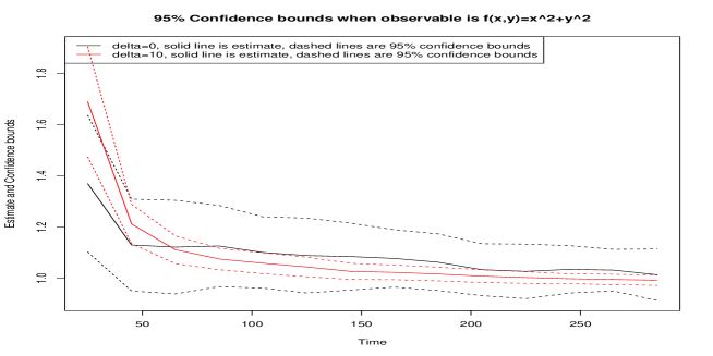
We present three different examples. In the first example we pick the potential and the observable . These dynamics was also considered in [23]. We remark here that the quantity is the long-time mean-square displacement of the process . In Figures 1 and 2 we see confidence bounds for . It is clear the adding irreversibility not only speeds up convergence to equilibrium, but it also results in significant reduction in the variance. In Figure 1 we compare the reversible case (i.e., with ) with the irreversible case with . Then, in Figure 2, we have also included the case . For the particular test case, the confidence bounds are even tighter when when compared to . This result illustrates Theorem 2.3 and Theorem 2.7.
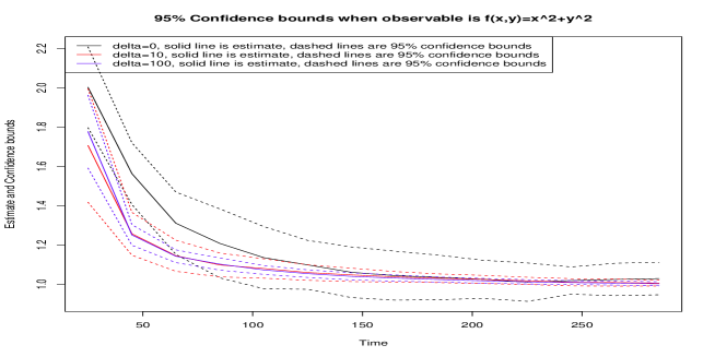
For illustration purposes, we present in Table 1, variance estimates for different values of and time horizons in the set-up of Figure 2. It is noteworthy that the variance reduction for this particular example is about two orders of magnitude.
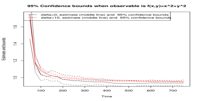
In the second example we pick again a bimodal potential and the observable . In Figure 3 we see confidence bounds for . In Table 2, we present numerical data for the variance estimates that are illustrated in Figure 3. Again, we see variance reduction and it is at the order of about two magnitudes.
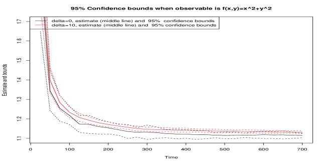
In the third example we pick the potential
Due to the somewhat complex form of , we have also plotted in Figure 4 its phase portrait.

We see that it has two local minima at , two saddle points at and at and a local maximum at .
We consider again the observable . In Figure 5 we see confidence bounds for . In Table 3, we present numerical data for the variance estimates that are illustrated in Figure 5. Again, we see variance reduction and it is at the order of about one magnitude when the irreversible parameter is .
We conclude this section with a remark on the optimal choice of irreversibility. Theorem 2.3 suggests that in the generic situation, perturbations of the form yield better results as the parameter increases. However, in practice the higher the is, the smaller the discretization step in the simulation algorithm should be, i.e., there is a trade-off to consider here. Thus it makes sense to look for the optimal perturbation and this could be formulated as a solution to a variational problem that involves minimizing the asymptotic variance of the estimator. Since, the asymptotic variance is inversely proportional to the second derivative of the rate function of the observable evaluated at , the variational problem to consider is basically maximization over vector fields that satisfy condition of the quantity (4.12) under the constraint (4.13). We plan to investigate this question in a future work.
6. Conclusions
In this article we have considered the problem of estimating the expected value of a functional of interest using as estimator the long time average of a process that has as its invariant distribution the target measure. We have argued using large deviations theory, both theoretically and numerically, that adding an appropriate drift to the dynamics of a reversible Langevin equation, results in smaller asymptotic variance for the time average estimator. We characterize when observables do not see their variance reduced in terms of a precise non-linear Poisson equation.
References
- [1] Y. Amit and U. Grenander, Comparing sweeping strategies for stochastic relaxation, Journal of Multivariate Analysis, Vol. 37, (1991), pp. 197-222.
- [2] S. Asmussen and P.W. Glynn, Stochastic Simulation, Springer, 2007.
- [3] K.A. Athreya, H. Doss and J. Sethuraman, On the convergence of the Markov chain simulation method, Annals of Statistics, Vol. 24, (1996), pp. 69-100.
- [4] C. Barbarosie, Representation of divergence-free vector fields, Quarterly of Applied Mathematics, Vol. 69, (2011), pp. 309–316.
- [5] M. Bedard and J.S. Rosenthal, Optimal Scaling of Metropolis Algorithms: Heading Towards General Target Distributions, Canadian Jounral of Statistics, Vol. 36, Issue 4, (2008), pp. 483-503.
- [6] J. Bierkens, Non-reversible Metropolis-Hastings. Preprint (2014), arxiv.org/abs/1401.8087
- [7] P. Constantin, A. Kiselev, L. Ryshik and A. Zlatos, Diffusion and mixing in fluid flow Annals of Mathematics, Vo. 168 (2008), pp. 643-674.
- [8] F. Den Hollander, Large deviations, American Mathematical Society, Providence, RI, 2000.
- [9] P. Diaconis, S. Holmes and R. Neal, Analysis of a nonreversible Markov chain sampler, Annals of Applied Probability, Vol. 10, (2010), pp. 726-752.
- [10] P. Diaconis and L. Miclo, On the spectral analysis of second-order Markov chains, submitted, (2013).
- [11] M.D. Donsker and S.R.S. Varadhan, Asymptotic evaluation of certain Markov process expectations for large times, I, Communications Pure in Applied Mathematics, Vol. 28, (1975), pp. 1-47, II, Communications on Pure in Applied Mathematics, Vol. 28, (1975), pp. 279–301, and III, Communications on Pure in Applied Mathematics, Vol. 29, (1976), pp. 389-461.
- [12] A. Douglis and L. Nirenberg, Interior estimates for elliptic systems of partial differential equations. Communications Pure in Applied Mathematics, Vol. 8, (1975), pp. 503-538.
- [13] N. Plattner, J.D. Doll, P. Dupuis, H. Wang, Y. Liu, and J.E. Gubernatis. An infinite swapping approach to the rare-event sampling problem. J. of Chemical Physics, Vol. 135, (2011), pp. 134111.
- [14] P. Dupuis, Y. Liu, N. Plattner, and J. D. Doll, On the Infinite Swapping Limit for Parallel Tempering. SIAM Multiscale Modeling and Simulation, Vol. 10, Issue 3, (2012), pp. 986-1022.
- [15] B. Franke, C.-R. Hwang, H.-M. Pai, and S.-J. Sheu, The behavior of the spectral gap under growing drift, Transactions of the American Mathematical Society, Vol 362, No. 3 (2010), pp. 1325-1350.
- [16] A. Frigessi, C.R. Hwang, S.J. Sheu and P. Di Stefano, Convergence rates of the Gibbs sampler, the Metropolis algorithm, and their single-site updating dynamics, Journal of Royal Statistical Society Series B, Statistical Methodology, Vol. 55, (1993), pp. 205-219.
- [17] A. Frigessi, C.R. Hwang and L. Younes, Optimal spectral structures of reversible stochatic matrices, Monte Carlo methods and the simulation of Markov random fields, Annals of Applied Probability, Vol. 2, (1992), pp. 610-628.
- [18] J. Gärtner, On large deviations from the invariant measure, Theory of probability and its applications, Vol. XXII, No. 1, (1977), pp. 24-39.
- [19] W.R. Gilks and G.O. Roberts, Strategies for improving MCMC, Monte Carlo Markov Chain in practice, Chapman and Hall, Boca Raton, FL, (1996), pp. 89-114.
- [20] C.R. Hwang, S.Y. Hwang-Ma and S.J. Sheu, Accelerating Gaussian diffusions. The Annals of Applied Probability Vol. 3, (1993) pp. 897-913.
- [21] C.R. Hwang, S.Y. Hwang-Ma and S.J. Sheu, Accelerating diffusions, The Annals of Applied Probability, Vol 15, No. 2, (2005), pp. 1433-1444.
- [22] T. Kato, Perturbation theory of linear operators, New York, 1969.
- [23] T. Lelievre, F. Nier and G.A. Pavliotis, Optimal non-reversible linear drift for the convergence to equilibrium of a diffusion, CJournal of Statistical Physics, 152(2), (2013), pp. 237-274.
- [24] A. J. Majda and P. R. Kramer, Simplified models for turbulent diffusion: Theory, numerical modelling and physical phenomena, Physics Reports, 314 (4-5), (1999), pp. 237-574.
- [25] S. Meyn and R.L. Tweedie, Markov Chains and Stochastic Stability, Cambridge University Press, Second Edition, 2009.
- [26] A. Mira, Ordering and improving the performance of Monte Carlo Markov chains, Statist. Sci., Vol. 16, No. 4, (2001), pp. 340-350.
- [27] A. Mira and C. J. Geyer, On non-reversible Markov chains, In Monte Carlo methods, Volume 26 of Fields Inst. Commun, Amer. Math. Soc., Providence, RI, (2000), pp. 95-110.
- [28] R.M. Neal, Improving asymptotic variance of MCMC estimators: Non-reversible chains are better, Techincal report, No. 0406, Department of Statistics, University of Toronto, 2004.
- [29] K.L. Mergessen and R.L. Tweedie, Rates of convergence of the Hastings and Metropolis algorithms, Annals of Statistics, Vol. 24, (1996), pp. 101-121.
- [30] P.H. Peskun, Optimum Monte-Carlo Sampling Using Markov Chains, Biometrika, Vol. 60, No. 3 (1973), pp. 607-612.
- [31] R. Pinsky, The I-function for diffusion processes with boundaries, The Annals of Probability, Vol. 13, No. 3, (1985), pp. 676-692.
- [32] G.O. Roberts and J.S. Rosenthal, General state space Markov Chain and MCMC algorithms, Probability Surveys, Vol. 1, (2004), pp. 20-71.
- [33] R.T. Rockafellar, Convex Analysis, Princeton Landmarks in Mathematics and Physics, (1970).
- [34] Y. Sun, F. Gomez, and J. Schmidhuber, Improving the Asymptotic Performance of Markov Chain Monte- Carlo by Inserting Vortices. In Advances in Neural Information Processing Systems Vol. 23, (2010), pp. 2235 2243.
- [35] L. Tierney, A Note on Metropolis-Hastings Kernels for General State Spaces, The Annals of Applied Probability, Vol. 8, No. 1 (1998), pp. 1-9.