Stochastic resonance in the two-dimensional $q$-state clock models

Abstract

We numerically study stochastic resonance in the two-dimensional $q$-state clock models from $q=2$ to $7$ under a weak oscillating magnetic field. As in the mean-field case, we observe double resonance peaks, but the detailed response strongly depends on the direction of the field modulation for $q\geq 5$ where the quasiliquid phase emerges. We explain this behavior in terms of free-energy landscapes on the two-dimensional magnetization plane.

I Introduction

A weak input signal can be amplified by noise. This is called stochastic resonance (SR) and there has been a vast amount of theoretical and experimental studies about this phenomenon Gammaitoni et al. (1998). For a system with a single degree of freedom, SR can be illustrated by a particle trapped in a double-well potential but constantly hit by random noise: The particle inside one minimum moves to the other due to the noise, and this happens with a characteristic time scale $\tau$ denoted by the relaxation time. If we apply weak force that oscillates with frequency $f\sim\tau^{-1}$, which is termed time-scale matching condition, the particle can jump over the potential barrier back and forth in a periodic manner, amplifying the input force.

In many practical situations, the noise is given by thermal contact with a heat bath, and $\tau$ thus depends on temperature $T$ Néda (1995); Leung and Néda (1998). For a system with a single degree of freedom, $\tau$ is described by the simple Kramer rate Nicolis and Nicolis (2000) which diverges exponentially at $T=0$. As a result, if we consider the response as a function of $T$, the time-scale matching condition is usually fulfilled at a single point, and multiple resonance peaks are observable only when the dynamics has certain symmetry Vilar and Rubi (1997). For a system with many degrees of the freedom, on the other hand, $\tau$ is not necessarily explained in that way: If the system undergoes a continuous phase transition at $T=T_{c}$, for example, $\tau$ diverges at this critical point. In other words, $\tau^{-1}$ has a nonzero value over the whole temperature region except at $T_{c}$. Therefore, as long as $f$ is low enough, the matching condition can be satisfied once above $T_{c}$ and once below $T_{c}$, so the resonance will take place twice as $T$ varies from zero to infinity. The prediction of double peaks has been confirmed in various many-body systems under periodic perturbations, including classical spin systems Néda (1995); Kim et al. (2001); Baek and Kim (2012) as well as a quantum-mechanical case Han et al. (2012). However, most of these systems share one common feature that they undergo spontaneous symmetry breaking in the absence of external perturbations. Our question in this study is how the response changes if a system possesses the quasi-long-range order without spontaneous symmetry breaking, and the two-dimensional (2D) $q$-state clock model José et al. (1977); *elit can be the best candidate to systematically investigate this problem. This model has played an important role in a 2D melting scenario Strandburg (1988), and some experimental studies suggest a connection of this model to domain pattern in ferroelectric materials Chae et al. (2012).

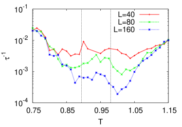
Figure 1: (Color online) Relaxation time $\tau$ of the five-state clock model in equilibrium at $\mathbf{h}=0$, obtained from the normalized autocorrelation function of $m$ (see Ref. Kim et al. (1997)). The temperature $T$ is given in units of $J/k_{B}$, where $k_{B}$ is the Boltzmann constant, and the vertical lines indicate $T_{c1}$ and $T_{c2}$ in the thermodynamic limit, respectively, estimated in Ref. Borisenko et al. (2011). As the system size increases, $\tau^{-1}$ vanishes in the quasiliquid phase between $T_{c1}$ and $T_{c2}$, where $\mathbf{m}=me^{i\phi}$ may freely wander around in the angular direction.

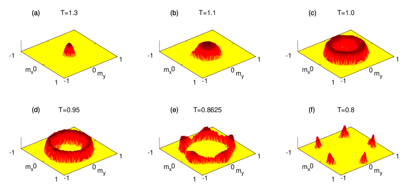
Figure 2: (Color online) Free-energy landscapes on the magnetization plane, drawn upside down for the five-state clock model with size $N=80\times 80$ (see text for details).

Let us review some equilibrium properties of this model. The Hamiltonian of the $q$-state clock model in the $L\times L$ square lattice is written as

$$H=-J\sum_{\left<j,k\right>}\mathbf{S}_{j}\cdot\mathbf{S}_{k}-\mathbf{h}\cdot\sum_{j}\mathbf{S}_{j},$$ (1)

where $J$ is a coupling constant, $\sum_{\left<j,k\right>}$ runs over the nearest neighbor pairs and $\mathbf{h}$ is an external magnetic field. Each spin $\mathbf{S}_{j}$ at site $j$ has a discrete angle $\theta_{j}=2\pi n_{j}/q$ with $n_{j}=0,1,2,\ldots,q-1$. If $q=2$, the model reduces to the Ising model, and it approaches the $XY$ model as $q\rightarrow\infty$. The magnetization is given as a 2D vector $\mathbf{m}=N^{-1}\sum_{j}\mathbf{S}_{j}$, where $N\equiv L^{2}$ is the total number of spins, and it can also be written as a complex number $me^{i\phi}=N^{-1}\sum_{j}e^{i\theta_{j}}$ with $m\equiv|\mathbf{m}|$. Suppose that the field $\mathbf{h}$ is absent. For $q<5$, the system undergoes a single order-disorder transition and we may well expect double resonance peaks Néda (1995); Kim et al. (2001); Baek and Kim (2012). On the other hand, if $q\geq 5$, there appear two infinite-order phase transitions, one at $T_{c1}$ and the other at $T_{c2}(>T_{c1})$ Baek and Minnhagen (2010); Baek et al. (2013). In the disordered phase at $T>T_{c2}$, the spins are randomly rotated by thermal fluctuations to one of the $q$ possible directions so that two spins are not much correlated if placed just a few lattice spacings apart. It is obvious that $m$ vanishes in this phase. When $T<T_{c1}$, on the other hand, almost all the spins point in the same direction, yielding nonzero $m$. In this ordered phase, thermal fluctuations are so weak that a spin can only individually deviate from the preferred direction every once in a while. It implies that there is no appreciable collective mode and we again find short-ranged correlation in spin fluctuations. The intermediate phase between $T_{c1}$ and $T_{c2}$ is actually more interesting than the other two surrounding it, because the spin-spin correlation decays algebraically with a diverging correlation length $\xi\rightarrow\infty$. The spin relaxation time $\tau$ also diverges because $\tau\sim\xi^{z}$ with a dynamic critical exponent $z>0$. This intermediate phase is sometimes dubbed quasiliquid due to the nontrivial correlations in space and time. Since $\tau^{-1}$ is zero in the quasiliquid phase (Fig. 1), we deduce that the time-scale matching condition can be satisfied below $T_{c1}$ and above $T_{c2}$, but not in between.

It is instructive to see the free-energy landscape $f(\mathbf{m})$ in the 2D magnetization plane (Fig. 2). It can be estimated as $f(\mathbf{m})\propto-k_{B}T\ln{p(\mathbf{m})}$, where $k_{B}$ is the Boltzmann constant and $p(\mathbf{m})$ means the probability to observe $\mathbf{m}$ in Monte Carlo (MC) simulations. We have obtained Fig. 2 by simulating the model on a $80\times 80$ square lattice, where both $J$ and $k_{B}$ are set to unity. For better visualization, the landscapes are drawn upside down so that a free-energy minimum appears as a peak. In the disordered phase at $T>T_{c2}$, the free-energy landscape has a global minimum at the center [Fig. 2(a)], which implies $m=0$ in the thermodynamic limit as explained above. One should note that the nonzero $m$ in the disordered and the quasiliquid phases is a finite-size effect which eventually vanishes as $N\rightarrow\infty$. In the disordered phase, $\mathbf{m}$ can take any angle $\phi$ between zero and $2\pi$, and the minimum gets broader as $T$ decreases [Fig. 2(b)]. It is important that the transition at $T_{c2}$ is not involved with spontaneous symmetry breaking [Figs. 2(c) and 2(d)], and the breaking happens only when $T$ is lowered further down to $T_{c1}$ [Figs. 2(e) and 2(f)]. When the system is perturbed slightly from a minimum of this free-energy landscape $f(\mathbf{m})$, we expect $d\mathbf{m}/dt\propto-\partial f/\partial\mathbf{m}$ Baek and Kim (2012). In other words, if the minimum is approximated as $f(\mathbf{m})\approx\frac{1}{2}\kappa|\mathbf{m}|^{2}$ in the high-temperature phase, our guess is that the coefficient $\kappa$ will be inversely proportional to the relaxation time $\tau$ since $d\mathbf{m}/dt\propto-\kappa\mathbf{m}$. Such a relation is well substantiated in Fig. 3. If we further extend this observation to lower temperatures, the shapes of the landscapes immediately suggest the existence of two different time scales, i.e., one in the radial direction and the other in the angular direction, which we denote by $\tau_{\parallel}$ and $\tau_{\perp}$, respectively. Even if a time-dependent external field is applied, as long as it is weak enough, the free-energy picture can still provide us with qualitative understanding. We therefore expect from Fig. 2 that the SR behavior will depend on the modulating direction of $\mathbf{h}$ when $q\geq 5$ and $T<T_{c2}$.

Figure 3: Comparison between the inverse relaxation time, measured from the autocorrelation of $m$, and the curvature of the free-energy landscape (see Fig. 2) near its minimum with varying $T$. Each data point represents a different $T$ in the high-temperature phase ($1.1\leq T\leq 1.2$) for the system of the size $L=80$. The error bar is smaller than the symbol size.

This speculation is readily confirmed by our numerical calculations: By measuring correlation between $\mathbf{m}$ and $\mathbf{h}$ as will be detailed below, we observe the followings: When a time-varying field $\mathbf{h}$ is applied in the direction of $\mathbf{m}$, we find that the transition point $T_{c2}$ is sandwiched between two SR peaks as in the Ising case Néda (1995); Kim et al. (2001); Baek and Kim (2012), though the one below $T_{c2}$ is broadened all the way down to $T_{c1}$. If the driving field $\mathbf{h}$ is orthogonal to $\mathbf{m}$, the behavior becomes radically different because it is the whole quasiliquid phase rather than a single point that is surrounded by two SR peaks. We first begin with explaining our numerical method in the next section and then present the results in Sec. III. With discussing physical implications of our results, we conclude this work in Sec. IV.

II Numerical method

In case of the Ising model ($q=2$), it is a common practice to use the kinetic Glauber-Ising dynamics Glauber (1963) when one studies its behavior slightly out of equilibrium Leung and Néda (1998); Kim et al. (2001). It is worth noting that this approach has achieved qualitative agreements with experimental observations such as dynamic hysteresis Chakrabarti and Acharyya (1999). We need to generalize the Glauber dynamics for simulating the $q$-state clock model Baek and Kim (2012), the result of which essentially corresponds to the heat-bath algorithm among MC methods Loison et al. (2004); *newman. Although MC algorithms are not meant to simulate dynamic properties, it has been widely accepted that they can effectively describe real dynamics as long as equipped with a local update rule and a small acceptance ratio Nowak et al. (2000); *mcdynamics. So our algorithm works as follows: We randomly choose a spin, say, $\mathbf{S}_{j}$ with $\theta_{j}=2\pi n_{j}/q$, and calculate how much the energy would change if the angle was switched to $\theta_{j}^{\prime}=2\pi n_{j}^{\prime}/q$. Denoting this amount of change by $\Delta E(n_{j}^{\prime})$, the probability to choose $n_{j}^{\prime}$ as its next value is given as $p(n_{j}^{\prime})\propto\exp[-\Delta E(n_{j}^{\prime})/T]$ with a normalization condition $\sum_{n_{j}^{\prime}}p(n_{j}^{\prime})=1$.

The underlying geometry is the $L\times L$ square lattice with periodic boundary conditions, the size of which varies between $L=40$ and $160$. The time $t$ in MC simulations is measured in units of one MC time step which corresponds to $N$ MC tries for spin update. We will fix the field amplitude $h_{0}=10^{-2}$ and frequency $f=10^{-3}$, respectively, throughout this work. As mentioned above, we may consider two different field directions: Since the angle of $\mathbf{m}$ is denoted as $\phi$, the field in the parallel direction is written as $\mathbf{h}_{\parallel}(t)=h_{0}\cos{2\pi ft}(\cos{\phi},\sin{\phi})$, while in the perpendicular direction it is written as $\mathbf{h}_{\perp}(t)=h_{0}\cos{2\pi ft}(-\sin{\phi},\cos{\phi})$. Since $\phi$ is also time-dependent, we need to measure it at the beginning of each period to adjust the field direction, but it should be kept fixed within the period. We are going to apply either $\mathbf{h}_{\parallel}$ or $\mathbf{h}_{\perp}$ to the system and compare the responses. We point out that an external field ${\mathbf{h}}$ in a fixed direction can be decomposed into two components (parallel and perpendicular to ${\mathbf{m}}$) and the system’s response contains contributions from both components. We drive the system either by $\mathbf{h}_{\parallel}$ or by $\mathbf{h}_{\perp}$ only to identify physical mechanism of the resonance behavior more clearly in comparison with the temperature-dependent free-energy landscape in Fig. 2. Our main observable is defined as

$$D\equiv\left\langle\frac{1}{h_{0}\Lambda}\int_{n\Lambda}^{(n+1)\Lambda}\mathbf{m}\cdot\mathbf{h}~{}dt\right\rangle,$$ (2)

where the integral is over one period $\Lambda\equiv f^{-1}$ and the bracket means the average over $n\in[101,900]$ with the transient behavior in early times ($n\in[0,100]$) neglected. In one limiting case where $T\rightarrow\infty$, $D$ should be identically zero since $m$ vanishes there. In the other limiting case where $T\rightarrow 0$, $\mathbf{m}$ is frozen regardless of the small perturbation $\mathbf{h}$ so that the integral of cosine over one period yields zero again. Only when $\mathbf{m}$ runs closely after $\mathbf{h}$, the integrand gives positive contribution on average, and we interpret a large value of $D$ as signaling the stochastic resonance behavior. At the same time, one should note that $\mathbf{m}\perp\mathbf{h}$ may also induce vanishingly small $D$ even if $\mathbf{m}$ does vary in time.

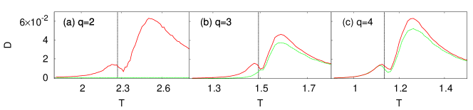
Figure 4: (Color online) Responses for $q<5$, where the solid (red) and dashed (green) curves show results under $\mathbf{h}_{\parallel}$ and $\mathbf{h}_{\perp}$, respectively. (a) When $q=2$, the system can respond only to $\mathbf{h}_{\parallel}$. (b) When $q=3$ or (c) $q=4$, double SR peaks appear in any of the field directions. The vertical dotted lines indicate the equilibrium critical points in the thermodynamic limit when the field is absent.

Figure 5: (Color online) The solid (red) lines represent $m$ for $q=2$, and the sinusoidal dashed (green) lines show the normalized external field, $\cos 2\pi ft$. (a) When $T$ is low, the system is frozen at a symmetry-broken state. (b) As $T$ increases, $m$ begins to fluctuate but the amplitude is small because it is trapped in a narrow free-energy minimum. (c) The strongest response is found around the resonance peak above $T_{c}$ where $m(t)$ moves between the positive and negative sides. (d) If $T$ increases further, the free-energy minimum at the origin ($m=0$) gets narrow and the resonance is thus suppressed.

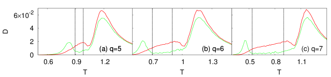
Figure 6: (Color online) Double SR peaks for $q\geq 5$, where the solid (red) and dashed (green) lines mean the results under $\mathbf{h}_{\parallel}$ and $\mathbf{h}_{\perp}$, respectively. The equilibrium critical points in the thermodynamic limit are represented as the vertical dotted lines. While strong responses are found below and above $T_{c2}$ under $\mathbf{h}_{\parallel}$, the quasiliquid phase shows little $D$ under $\mathbf{h}_{\perp}$ so the left peak is located below $T_{c1}$. Note that $T_{c1}$ ($T_{c2}$) tends to be underestimated (overestimated) for finite $N$.

III Results

In this section, we present MC results obtained only for $L=80$, because the qualitative features remain unaltered for larger systems and there is little size dependence in peak heights as well.

If $q<5$, the system undergoes a single continuous phase transition. Therefore, the observable $D$ shows the expected double-peak structure, one below and the other above $T_{c}$ when $\mathbf{h}_{\parallel}$ is applied (Fig. 4). Even though $\mathbf{h}_{\perp}$ has no physical meaning in the Ising case ($q=2$), it induces qualitatively the same responses as $\mathbf{h}_{\parallel}$ does when $q=3$ or $q=4$. It is notable that the two peaks are highly asymmetric in each plot, which means that the system amplifies the signal better at the second peak above $T_{c}$ (Fig. 5). This asymmetry is characteristic of a low-dimensional system, in contrast to the mean-field (MF) case Baek and Kim (2012): In the MF case with a given field frequency $f$, the response is fully specified by $\tau$. Since each of the double peaks is characterized by the same condition that $\tau\sim f^{-1}$, the peak height is accordingly the same as well. Returning back to the 2D case, we see that the asymmetry is actually plausible because the system is more susceptible in the disordered phase. It is well-known that the static susceptibility $\chi$ around $T_{c}$ behaves as $\chi_{\pm}\sim\Gamma_{\pm}|T-T_{c}|^{-\gamma}$, where the subscript means the sign of the reduced temperature $(T-T_{c})/T_{c}$, and $\gamma$ is a critical exponent of the model. A prediction from the renormalization-group theory is that the amplitude ratio between $\Gamma_{+}$ and $\Gamma_{-}$ is universal, whereas they are not individually. The universal amplitude ratio is exactly calculated as $\Gamma_{+}/\Gamma_{-}=37.6936520\ldots$ for $q=2$ and $q=4$ Barouch et al. (1973); *delfino, and estimated as $\Gamma_{+}/\Gamma_{-}\approx 13.86(12)$ for $q=3$ Shchur et al. (2008). It is reasonable to guess that a relevant factor to the peak height will be $\left<\Delta m\right>=\sqrt{\left<m^{2}\right>-\left<m\right>^{2}}\propto\chi^{1/2}$. In other words, our guess is that the ratio between the peak heights $D^{\ast}_{+}/D^{\ast}_{-}$ is roughly proportional to $(\chi_{+}/\chi_{-})^{1/2}\sim(\Gamma_{+}/\Gamma_{-})^{1/2}$ so that $\zeta\equiv(D^{\ast}_{+}/D^{\ast}_{-})^{-1}(\Gamma_{+}/\Gamma_{-})^{1/2}$ yields similar values when $q$ varies between $2$ and $4$. Although this argument is not meant to be exact and the estimates of $D^{\ast}_{+}/D^{\ast}_{-}$ are not precise either, this explains some part of the observation because we indeed find $\zeta=1.32(12)$, $1.31(7)$, and $1.44(4)$ for $q=2,3$, and $4$, respectively. Moreover, these values are comparable to the MF result $\zeta_{\rm MF}=\sqrt{2}=1.414\ldots$ since we already know $D^{\ast}_{+}/D^{\ast}_{-}=1$ and the Landau theory predicts $\Gamma_{+}/\Gamma_{-}=2$.

It is straightforward to perform the same simulations for $q\geq 5$, but the behavior is rather different depending on the field direction as expected (Fig. 6). The response is insensitive to the direction in the disordered phase since $\mathbf{m}$ has no meaningful direction with vanishingly small magnitude. Below $T_{c2}$, however, the dependence on the field direction is clearly visible, which can be understood by using the free energy landscape (Fig. 2), provided that the field is so weak that the system remains close to equilibrium. According to this picture, in the quasiliquid phase, there is no significant free-energy barrier in the angular direction: This implies very large $\tau_{\perp}$, whereas $\tau_{\parallel}$ remains always finite because the system is effectively confined in a free-energy well in the radial direction. This explains why the SR peak is observed only under $\mathbf{h}_{\parallel}$ in this phase. It is below $T_{c1}$ that the system experiences free-energy barriers in the angular direction. This barrier regulates the divergence of $\tau_{\perp}$, and a clear resonance peak is thereby developed under $\mathbf{h}_{\perp}$. For an arbitrary field direction, the response of the system is described as a combination of the results under $\mathbf{h}_{\parallel}$ and $\mathbf{h}_{\perp}$, because we are working in the linear-response regime. We have also measured peak height ratios when $q\geq 5$ for the sake of completeness: Under $\mathbf{h}_{\parallel}$, we estimate $D^{\ast}_{+}/D^{\ast}_{-}$ as $3.55(11)$, $3.4(2)$, and $3.2(1)$ for $q=5,6$, and $7$, respectively. If we apply $\mathbf{h}_{\perp}$ instead, the estimates of $D^{\ast}_{+}/D^{\ast}_{-}$ now read $2.91(7)$, $2.6(1)$, and $2.5(1)$, respectively. It is interesting that $q=6$ and $7$ are so similar in this respect that the values in either direction are on top of each other within the errorbars.

IV Conclusion

Figure 7: Spin configuration of the 2D clock model in the large-$q$ limit quenched from $T=\infty$ to $T=0$. Each spin direction $\theta_{j}$ is expressed as brightness proportional to $\sin^{2}2\theta_{j}$.

We have investigated responses of the 2D $q$-state clock system under external oscillating fields. Double resonance peaks are found below and above the unique critical point $T_{c}$ for $q<5$, and the peak positions are not sensitive to the field direction. For $q\geq 5$, however, the emergence of the quasiliquid phase in 2D makes the situation more complicated than the MF analysis in that the resonance behavior crucially depends on the field direction, especially when $T<T_{c2}$. We have qualitatively explained this difference by using the free energy landscape. Of course, the free-energy argument implies that we have restricted ourselves to the linear-response regime, which loses validity as the applied field becomes stronger.

We may also interpret the directional dependence in the quasiliquid phase in the context of liquid crystal (LC) de Gennes and Prost (1993): Suppose that each LC molecule carries a small electric dipole moment and can be described as an $XY$-typed spin variable. If a thin LC film is exposed to linearly polarized light, the oscillating electric field interacts with each electric dipole, and the periodically driven dipole in turn emits electromagnetic waves as a response. Our observation in this work suggests how the response will depend on the relative orientation between the dipole moment and the polarization of the incident light: If they are perpendicular to each other, for example, the molecule will respond to the input with a large phase delay due to the continuous symmetry, as indicated by small $D$. As a consequence, secondary wave will interfere destructively with the primary one. In addition, when LC is placed between two crossed polarizers, the so-called Schlieren texture de Gennes and Prost (1993) captures spatial variations in orientations of the LC molecules. In a simple thought experiment where these polarizers are taken into account, as the direction $\phi$ of LC rotates from zero to $2\pi$, the final intensity of light through the second polarizer will have four minima at $\phi=0,\pi/2,\pi$, and $3\pi/2$. By numerically simulating the quasiliquid phase of a 2D clock model with very large $q$, we illustrate a possible optical image in Fig. 7, which precisely reproduces a typical Schlieren texture in real experiments.