A Calculus of Located Entities

Abstract

We define BioScape^L, a stochastic pi-calculus in 3D-space. A novel aspect of BioScape^L is that entities have programmable locations. The programmer can specify a particular location where to place an entity, or a location relative to the current location of the entity. The motivation for the extension comes from the need to describe the evolution of populations of biochemical species in space, while keeping a sufficiently high level description, so that phenomena like diffusion, collision, and confinement can remain part of the semantics of the calculus. Combined with the random diffusion movement inherited from BioScape, programmable locations allow us to capture the assemblies of configurations of polymers, oligomers, and complexes such as microtubules or actin filaments.

Further new aspects of BioScape^L include random translation and scaling. Random translation is instrumental in describing the location of new entities relative to the old ones. For example, when a cell secretes a hydronium ion, the ion should be placed at a given distance from the originating cell, but in a random direction. Additionally, scaling allows us to capture at a high level events such as division and growth; for example, daughter cells after mitosis have half the size of the mother cell.

1 Introduction

Our earlier work on BioScape[11] was motivated by the need to visualize the evolution of species in 3D space. The simulator of BioScape randomly places initial distributions of entities within specified confinement areas. However, while BioScape naturally captures a large family of wet-lab experiments, it does not have the ability to describe the assembly of entities into compound structures such as dimers, polymers, oligomers, etc. In order to describe the composition of such structures from smaller components, we introduce a new calculus where an entity’s location can be programmed. The long-term goal of our research program is to create programming platforms to describe complex 3D landscapes, where agents interact with the environment. Applications of such modeling platforms include simulating intracellular viral traffic, and designing multifunctional antibacterial surfaces that prevent or minimize infection while maximizing tissue growth.

In this paper we define BioScape^L, a stochastic $\pi$-calculus in 3D-space with programmable locations. It builds on BioScape[11] by adding three new features: programmable entity’s location, random translation and scaling. As we just mentioned, programmable locations allow the programmer to specify the location of new entities, either by describing an absolute location in the global frame, or by specifying a location relative to the current location of the generating entity. Random translation lets the programmer describe a distance from the original position where to place the new entity without specifying an absolute or relative location. For example a random translation from point p of 1cm will place the new entity’s barycentre somewhere on the 1cm radius sphere around p. Finally, scaling enables the creation of new entities whose shape is obtained by resizing the shape of the original entity. The key aspect of all three extensions is their high level nature. The placement of new objects in space needs to account for confinement and collision, which in BioScape^L are part of the semantics of the calculus, unlike in low level calculi, where they are a burden to the programmer.

As we observed before, dynamic spatial arrangement of components is useful in representing assembly of polymers such as actin filaments and cytoskeletal microtubules. Microtubules are part of the cytoskeleton of eukaryotic cells, and form roads on which organelles ride on their way to the cell nucleus. Microtubules are hollow and formed with dimers of $\alpha$ and $\beta$ tubulin. They are anchored to a starting point around the Microtubules Organizing Center, and while the starting point is fixed, microtubules grow and shrink from the end piece. We now motivate the programmable entity’s location feature, by implementing a simplified model of microtubules polymerization in BioScape^L. Random translation and scaling are introduced later in Section 4.

val Cytosol:space =  cuboid(50.0,50.0,30.0) @ <1.0,2.0,24.0>
val step = 0.0,stepP = 0.1, r = 0.0, rP= 0.2
new MTConstruction@0.116,rP:ch(ch(),fl*fl*fl)

let MTPart()@Cytosol,stepP,sphere(1.0)=( new y@0.27,r:ch()
do ?MTConstruction(x,u); MTLeft(x)_glue(this,u)
or !MTConstruction(y,this); MTRight(y)_this
or mov.MTPart()_this )

and MTRight(rht:chan())@Cytosol,step,sphere(1.0) =
do delay@1.0; MTRight(rht)_this
or ?rht; MTPart()_this

and MTLeft(lft:chan())@Cytosol,step,sphere(1.0) =
( new z@0.27,r:ch()
do delay@1.0; MTLeft(lft)_this
or !MTConstruction(z,this); MTMiddle(lft,z)_this
or !lft; MTPart()_this
or ?lft;MTPart()_this )

and MTMiddle(rht1:chan(),lft1:chan())@Cytosol,
     step,sphere(1.0) =
do delay@1.0; MTMiddle(rht1,lft1)
or !lft1;MTLeft(rht1)_this

run (MTPart()_p1 | MTPart()_p2 |...| MTPart()_pN )

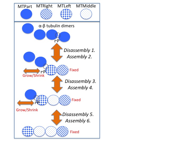
Figure 1: Microtubules polymerization

A motivating example

For our next example, microtubules polymerization, consider Fig. 1, containing the BioScape^L code as well as a graphical representation of the evolution of the system. Microtubules are dynamic tubulin polymers; although they are formed with dimers of $\alpha$ and $\beta$ tubulin, we simplify their structure in our example, and consider them as assembled starting from parts, MTPart, where a part is an $\alpha$-$\beta$ tubulin dimer. MTParts are scattered in the Cytosol. Microtubules have a start piece MTRight and an end piece MTLeft. Between the start (right) and the end (left) pieces there can be any number of MTMiddle pieces. While the start piece is fixed, microtubules grow and shrink from the end piece. In order to grow, a new MTPart becomes the new MTLeft, and the old MTLeft becomes an MTMiddle. Similarly the end piece can disassemble making the last MTMiddle the new MTLeft, and making the old MTLeft a free MTPart. The construction is done using private channels, similar to the process modeling of actin polymerization of [7], so that only adjacent pieces share channels. In this model, we assume that MTLeft, MTMiddle, and MTRight do not move, unless they become a free MTPart.

We assume an initial concentration of N MTPart’s placed in the Cytosol, implemented with a parallel composition of N copies of MTPart with barycentres p1, $\cdots$, pN in the run command at the end of the program.

The first line of code defines the space within which all the entities are enclosed. It is a cuboid whose bottom left vertex is the point (1.0,2.0,24.0). The second line defines four floating point constants which will be used to specify the step of the diffusion rate of the entities, and the radius of the channels. The diffusion rates are: step=0.0 for the components of the microtubules, i.e., MTLeft, MRight, and MTMiddle, since we assume that they do not move, and stepP=0.1 for MTParts, which are subject to brownian motion. The radius of a channel is the maximum distance between two entities synchronizing on that channel. Communications between entities forming microtubules requires radius r=0.0, specifying that communication can only happen upon contact. Instead, the radius rP specifies that for two entities to synchronize on channel MTConstruction, their closest points must be at most 0.2 units apart.

The expression new MTConstruction@0.116,rP:ch(ch(),fl*fl*fl) declares channel
MTConstruction, with stochastic rate 0.116, and radius rP. The stochastic rate is used by the simulation algorithm to determine the probability and the reaction time for synchronization on the channel. The type ch(ch(),fl*fl*fl) declares MTConstruction, as a channel on which the data exchanged are pairs whose first component is another channel and the second component is a triple of floating-point numbers.

In the rest of the program MTPart, MTRight, MTLeft, and MTMiddle are defined. Each definition has four components. Consider the case of MTPart, the Cytosol is the confinement area, where instances of MTPart can be located; stepP is the diffusion rate of an MTPart, sphere(1.0) is its shape, and the rest is a process describing the behavior of MTPart.

An MTPart can either synchronize with another MTPart and become MTRight and MTLeft respectively. It can also synchronize with an MTLeft, or move.

In more detail, for each instance of MTPart, a new private channel is created with new y@0.27,r, where y is the name of the channel. The stochastic reaction rate of the channel is 0.27, and the channel radius is r. MTPart can either do an input on channel MTConstruction, ?MTConstruction(x), or an output on the same channel, !MTConstruction(y).

Consider MTPart()_p1 | MTPart()_p2, representing MTPart’s at locations p1 and p2 respectively. If the closest points of the two parts are closer that rP, there can be a synchronization on channel MTConstruction. The entity MTPart()_p1 sends on channel MTConstruction the private channel name y and the position p1, and it becomes MTRight(y)_p1, whereas MTPart()_p2 receives y, and p1, on channel MTConstruction, binds y to x and u to p1, and it becomes MTLeft(y)_p3. Point p3, the result of glue(p2,p1), is such that MTLeft(y)_p3 and MTRight(y)_p1 are in contact with each other. MTLeft(y)_p3 shares the private channel y with MTRight(y)_p1. This evolution is shown in the picture at Fig. 1, by Assembly 2. Note that, ${\tt this}$ denotes the barycentre of the MTPart from which MTRight or MTLeft evolve. The metavariable ${\tt this}$ is an abstract reference to the runtime position of the generating entity; ${\tt this}$ is similar to the origin, ✠, of $3\pi$[8]. The position of an entity can be the result of an operation such as the sum of points or scalar product derived from the location of the originating entity (this).

The entity MTPart()_p1 can perform the move action, in which case a new point p4 placed randomly at distance stepP from p1 is generated, and MTPart()_p1 evolves into a new MTPart located at p4.

The entity MTRight can remain an MTRight with a delay prefix, or it can do an input action with the adjacent MTLeft with which it shares the channel rht and evolve into a MTPart placed in its original position (this). This corresponds to the final disassembling of the microtubule, shown in the picture in Fig. 1, by Disassembly 1. Notice that, in this case, there is no information sent on channel rht.

The entity MTLeft has a parameter lft, which is a channel private to MTLeft and the adjacent MTRight or MTMiddle. MTLeft has four alternative behaviors. It can remain an MTLeft with a delay prefix (first line of the definition). It can interact with a MTPart, by synchronizing on channel MTConstruction, and evolve into a MTMiddle with which it shares the private channel z for interactions, and to which it passes the private channel lft, shared with adjacent MTMiddle or MTRight. In other words, MTLeft(y)_p3 | MTPart()_p4 becomes MTMiddle(y,z)_p3 | MTLeft(z)_p5, where p5 is glue(p4,p3); see Assembly 4 and 6 in Fig. 1. In Assembly 4, the channel y is shared with the adjacent MTRight, whereas in Assembly 6, it is shared with the adjacent MTMiddle. MTLeft can also interact with a MTRight, by synchronizing on their private channel and disassemble; see Disassembly 1 in Fig. 1. Finally, MTLeft can interact with a MTMiddle on their private channel, and disassemble; see Disassembly 5 and 3 in Fig. 1. For example, consider MTMiddle(y,z)_p3 | MTLeft(z)_p5, the synchronization on private channel z makes MTMiddle(y,z)_p3 evolve into MTLeft(y)_p3. Alternatively, with the same synchronization, MTLeft(z)_p5 evolves into MTPart()_p5, becoming a free part.

The entity MTMiddle can remain an MTMiddle with a delay prefix, or it can synchronize with the adjacent MTLeft. As previously described, MTMiddle(y,z)_p3 evolves into MTLeft(y)_p3, which, in Disassembly 5, shares the channel y with an MTMiddle, whereas in Disassembly 3, it shares the channel y with the final MTRight.

2 BioScape^L: Syntax

$$P,Q \mathrel{::=}\boldsymbol{0}$$ Empty Process

$$\;\;\mid\;\;X(\delta)_{\delta}$$ Located Entity Instance

$$\;\;\mid\;\;P\mid Q$$ Parallel Composition

$$\;\;\mid\;\;(\nu a@{\delta,\delta}:{\tt chan}\{T\}).P$$ Restriction

$$M \mathrel{::=}\pi.P\;[+\;M]$$ Choice of Prefixed Process

$$\pi \mathrel{::=}\texttt{delay}@{\delta}$$ Delay

$$\;\;\mid\;\;!u(\delta)$$ Output

$$\;\;\mid\;\;?u(x)$$ Input

$$\;\;\mid\;\;\texttt{mov}$$ Move

$$N \mathrel{::=}{M\;\;\;\mid\;\;(\nu a@{\delta,\delta}:{\tt chan}\{T\}).N}$$ Restricted Choice

$$u \mathrel{::=}a\;\;\mid\;\;b\;\;\mid\;\;\cdots\;\;\mid\;\;x\;\;\mid\;\;y\;\;\mid\;\;\cdots$$ Identifiers

$$\delta \mathrel{::=}u\;\;\mid\;\;{\tt c}\;\;\mid\;\;{\tt this}\;\;\mid\;\;{\delta_{1},\ldots,\delta_{n}}\;\;\mid\;\;(\,)\;\;\mid\;\;\delta.i\;\;\mid\;\;{\tt op}(\delta)$$ Expressions

$$v \mathrel{::=}a\;\;\mid\;\;b\;\;\mid\;\;\cdots\;\;\mid\;\;{\tt c}\;\;\mid\;\;(\,)\;\;\mid\;\;{v_{1},\ldots,v_{n}}$$ Expression Values

$$T \mathrel{::=}{\tt chan}\{T\}\;\;\mid\;\;{\tt fl}\;\;\mid\;\;T_{1}\ast\cdots\ast T_{n}\;\;\mid\;\;\top$$ Expression Types

$$D \mathrel{::=}\emptyset\;\;\mid\;\;D,X(x:T)={N}^{\xi,\omega,\sigma}\quad\texttt{FV}(M)\subseteq\overline{x}$$ Entity Definitions

$$E \mathrel{::=}\emptyset\;\;\mid\;\;E,{a@{\tt r},{\tt rad}:{\tt chan}\{T\}}$$ Channel Declarations

$$\Gamma \mathrel{::=}\emptyset\;\;\mid\;\;\Gamma,X{:}T\;\;\mid\;\;\Gamma,u{:}T$$ Type Environment

Figure 2: Syntax of BioScape^L

The abstract syntax of BioScape^L extends that of BioScape [10], and it appears in Fig. 2. We assume a set of channel names, denoted by $a$, $b$, and a set of variables, denoted by $x$, $y$, and the metavariable ${\tt c}$ for real numbers. We will also use ${\tt r}$ for the stochastic rate, and ${\tt rad}$ to specifying the radius of channels, both ${\tt r}$, and ${\tt rad}$, are real numbers. Points, denoted by the metavariable $p$, are triples $({\tt c}_{1},{\tt c}_{2},{\tt c}_{3})$ of real numbers.

Expressions $\delta$ may be channel names, variables, real numbers, the metavariable ${\tt this}$, tuples of expressions, including the empty tuple $(\,)$, tuple selection $\delta.i$, and operators applied to expressions ${\tt op}(\delta)$. The metavariable ${\tt this}$ denotes the barycentre of the entity instance in which the expression is evaluated. Expression values, are either channel names, real numbers, or tuples of value. The BioScape^L types characterizing these values are: channel types, ${\tt chan}\{T\}$, specifying the type $T$ of the values sent on them; the type of real numbers, ${\tt fl}$; the type of tuples, $T_{1}\ast\cdots\ast T_{n}$, specifying the types $T_{i}$ of its components, and $\top$, which is the type of the empty tuple. Channels only used for synchronization, such as lft in Fig. 1 have type ${\tt chan}\{\top\}$.

The empty process is $\boldsymbol{0}$. By $X(\delta)_{\delta^{\prime}}$ we denote an instance of the entity defined by $X$, with actual parameter $\delta$ and positions $\delta^{\prime}$. The process $P\mid Q$ is the parallel composition of processes $P$ and $Q$. The process $(\nu a@\delta,\delta^{\prime}:{\tt chan}\{T\}).P$ defines the channel name $a$ with stochastic rate $\delta$, radius $\delta^{\prime}$, and type ${\tt chan}\{T\}$ in process $P$. As mentioned before, the radius is the maximum distance between entities in order to communicate through channel $a$, the reaction rate determines how long it takes for two entities to react given that they are close enough to communicate, and ${\tt chan}\{T\}$ states that $a$ is a channel for communicating values of type $T$.

The heterogeneous choice is denoted by $M$, where $\pi.P\;[+\;M]$ means $\pi.P\;\;\mid\;\;\pi.P\;+\;M$. Choices may have reaction branches and movement branches. The reaction branches are probabilistic (stochastic), since reactions are subject to kinetic reaction rates, while the movement branches are non-deterministic, since diffusion is always enabled. The prefix $\pi$ denotes the action that the process $\pi.P$ can perform. The prefix $\texttt{delay}@\delta$ is a spontaneous and unilateral reaction of a single process, where $\delta$ is the stochastic rate of the reaction. The prefix $!u(\delta)$ denotes the output of the value of $\delta$ on channel $u$, and the prefix $?u(x)$ denotes input on channel $u$ with bound variable $x$. The prefix mov denotes the movement of processes in space according to their diffusion rate $\omega$. We use standard syntactic abbreviations such as $\pi$ for $\pi.0$. The restricted choice, denoted by $N$, is a choice of prefixed processes $M$ with top level local channel definitions.

We denote by $D$ a global list of entity definitions. The clause $X(x:T)=N^{\xi,\omega,\sigma}$ defines entity $X$ with formal parameter $x$ of type $T$ to be the restricted choice $N$ with geometry $\xi,\omega,\sigma$, specifying a movement space $\xi$, a step $\omega$, and a shape $\sigma$. The restricted choice $N$ describes the behavior of $X$ with a choice of prefixed processes $M$, and the set of channels private to the entity $X$. The movement space $\xi$ is a 3D area where instances of $X$ are allowed to be located. The step $\omega\in\mathbb{R}_{\geq 0}$, is the distance that $X$ can move in a unit of time, and it corresponds to the diffusion rate of $X$; $\sigma$ is the three-dimensional shape (sphere, cube, etc.) of $X$, having a barycentre. The movement space for the empty process $\boldsymbol{0}$ is everywhere, the global space, and its movement step is 0. Each entity variable $X$ can be defined at most once in $D$, and the free variables of $N$, must be a subset of the variables $\overline{x}$. We also write $X(x)=(\pi.\pi^{\prime}.P)^{\xi,\omega,\sigma}$ as short for $X(x)=(\pi.Y(x))^{\xi,\omega,\sigma}$ and $Y(x)=(\pi^{\prime}.P)^{\xi,\omega,\sigma}$.

Free variables, FV, and free channel names, FN, of processes and choices can be defined in the usual way. The input prefix $?u(x)$, and the restriction $\nu a@\_$ are binders, and define the scope of the variable $x$, and the channel name $a$ respectively.

$E$ ranges over environments of channel name declarations. $a@{\tt r},{\tt rad}:{\tt chan}\{T\}$ defines channel name $a$ with rate ${\tt r}$, radius ${\tt rad}$ and type ${\tt chan}\{T\}$. The domain of $E$ is the set of channel names declared in $E$, and channel names are declared at most once in $E$.

$\Gamma$ ranges over type environments, which map entity names $X$ with the type of the parameter of the entity, channel names $a$ with channel types, and variables with their type.

In the concrete syntax of the example in Fig. 1, we used new instead of $\nu$; do-or instead of ${+}$, and !a, ?a, and chan() instead of !a(), ?a(), and ${\tt chan}\{\top\}$, when no value is exchanged,

3 BioScape^L: Semantics

We now introduce the static and dynamic semantics of BioScape^L. In Fig. 3 we define the well formed processes and definitions, and in Fig. 4, 5, and  6 the operational semantics of BioScape^L.

In Fig. 3 we define the rules for the judgements:

• $\Gamma\vdash\delta:T$, meaning, in the type environment $\Gamma$, the expressions $\delta$ has type $T$;

• $\Gamma\vdash R\ \diamond$, meaning, in the type environment $\Gamma$, $R$ is well formed, where $R$ is either a process $P$, a choice $M$ or a restricted choice $N$, and

• $\Gamma\vdash D\ \diamond$, meaning, in the type environment $\Gamma$, the list of definitions $D$ is well formed.

$$\scriptstyle{\textsc{(Ty.id)}}\ \displaystyle\frac{u{:}T\in\Gamma}{\Gamma\vdash u:T}\ \penalty 50\hskip 20.00003pt plus 0.5fil minus 5.0pt\scriptstyle{\textsc{(Ty.const)}}\ \displaystyle\frac{}{\Gamma\vdash{\tt c}:{\tt fl}}\ \penalty 50\hskip 20.00003pt plus 0.5fil minus 5.0pt\scriptstyle{\textsc{(Ty.this)}}\ \displaystyle\frac{}{\Gamma\vdash{\tt this}:{\tt fl}\ast{\tt fl}\ast{\tt fl}}\ \penalty 50\hskip 20.00003pt plus 0.5fil minus 5.0pt\scriptstyle{\textsc{(Ty.tuple)}}\ \displaystyle\frac{\Gamma\vdash\delta_{i}:T_{i}\quad(1\leq i\leq n)}{\Gamma\vdash{\delta_{1},\ldots,\delta_{n}}:T_{1}\ast\cdots\ast T_{n}}\ \penalty 50\hskip 20.00003pt plus 0.5fil minus 5.0pt\scriptstyle{\textsc{(Ty.empty)}}\ \displaystyle\frac{}{\Gamma\vdash(\,):\top}\ \penalty 50\hskip 20.00003pt plus 0.5fil minus 5.0pt\scriptstyle{\textsc{(Ty.sel)}}\ \displaystyle\frac{\Gamma\vdash\delta:T_{1}\ast\cdots\ast T_{n}\quad(1\leq i\leq n)}{\Gamma\vdash\delta.i:T_{i}}\ \penalty 50\hskip 20.00003pt plus 0.5fil minus 5.0pt\scriptstyle{\textsc{(Ty.op)}}\ \displaystyle\frac{{\tt typeOf}({\tt op})=(T_{1},T_{2})\quad\Gamma\vdash\delta:T_{1}}{\Gamma\vdash{\tt op}(\delta):T_{2}}\$$

$$\scriptstyle{\textsc{(Ty.nil)}}\ \displaystyle\frac{}{\Gamma\vdash\boldsymbol{0}\ \diamond}\ \penalty 50\hskip 20.00003pt plus 0.5fil minus 5.0pt\scriptstyle{\textsc{(Ty.inst)}}\ \displaystyle\frac{X{:}T\in\Gamma\quad\Gamma\vdash\delta:T\quad\Gamma\vdash\delta^{\prime}:{\tt fl}\ast{\tt fl}\ast{\tt fl}}{\Gamma\vdash X(\delta)_{\delta^{\prime}}\ \diamond}\ \penalty 50\hskip 20.00003pt plus 0.5fil minus 5.0pt\scriptstyle{\textsc{(Ty.par)}}\ \displaystyle\frac{\Gamma\vdash P\ \diamond\quad\Gamma\vdash Q\ \diamond}{\Gamma\vdash P\mid Q\ \diamond}\ \penalty 50\hskip 20.00003pt plus 0.5fil minus 5.0pt\scriptstyle{\textsc{(Ty.restr)}}\ \displaystyle\frac{\Gamma,a{:}{\tt chan}\{T\}\vdash R\ \diamond\quad\Gamma\vdash\delta:{\tt fl}\quad\Gamma\vdash\delta^{\prime}:{\tt fl}}{\Gamma\vdash(\nu a@\delta,\delta^{\prime}:{\tt chan}\{T\}).R\ \diamond}\ \penalty 50\hskip 20.00003pt plus 0.5fil minus 5.0pt\scriptstyle{\textsc{(Ty.out)}}\ \displaystyle\frac{u{:}{\tt chan}\{T\}\in\Gamma\quad\Gamma\vdash\delta:T\quad\Gamma\vdash P\ \diamond}{\Gamma\vdash!u(\delta).P\ \diamond}\ \penalty 50\hskip 20.00003pt plus 0.5fil minus 5.0pt\scriptstyle{\textsc{(Ty.in)}}\ \displaystyle\frac{u{:}{{\tt chan}\{T\}}\in\Gamma\quad\Gamma,x{:}T\vdash P\ \diamond}{\Gamma\vdash?u(x).P\ \diamond}\ \penalty 50\hskip 20.00003pt plus 0.5fil minus 5.0pt\scriptstyle{\textsc{(Ty.pref)}}\ \displaystyle\frac{\Gamma\vdash P\ \diamond}{\begin{array}[]{l}\Gamma\vdash\texttt{mov}.P\ \diamond\end{array}}\ \penalty 50\hskip 20.00003pt plus 0.5fil minus 5.0pt\scriptstyle{\textsc{(Ty.pref)}}\ \displaystyle\frac{\Gamma\vdash P\ \diamond\quad\Gamma\vdash\delta:{\tt fl}}{\begin{array}[]{l}\Gamma\vdash\texttt{delay}@\delta.P\ \diamond\end{array}}\ \penalty 50\hskip 20.00003pt plus 0.5fil minus 5.0pt\scriptstyle{\textsc{(Ty.choice)}}\ \displaystyle\frac{\Gamma\vdash M\ \diamond\quad\Gamma\vdash M^{\prime}\ \diamond}{\Gamma\vdash M\;+\;M^{\prime}\ \diamond}\ \penalty 50\hskip 20.00003pt plus 0.5fil minus 5.0pt\scriptstyle{\textsc{(Ty.defs)}}\ \displaystyle\frac{\Gamma\vdash D\ \diamond\quad\Gamma,x{:}T\vdash N\ \diamond}{\Gamma\vdash D,X(x:T)=N^{\xi,\omega,\sigma}\ \diamond}\$$

Figure 3: Well typed expressions, processes, and definitions

To define the type expressions, we assume a function ${\tt typeOf}$ such that ${\tt typeOf}({\tt op})=(T_{1},T_{2})$ means that the operator ${\tt op}$ takes a parameter of type $T_{1}$ and returns a value of type $T_{2}$. The rules for expressions are standard; notice that the type of ${\tt this}$ in rule (Ty.this) is a triple of floating-points representing 3D coordinates. An entity instance $X(\delta)_{\delta^{\prime}}$ is well formed (rule (Ty.inst)), if the actual parameter $\delta$ has the type associated with $X$ in the type environment, and if $\delta^{\prime}$ has the type of a 3D point. In rules (Ty.out) and (Ty.in) the channel identifier $u$ must have a channel type.

Definition 3.1 (BioScape^L Program, Initial Process, and Initial Configuration).

• A BioScape^L program is a triple $(D,E,P)$ such that $D$ is a collection of entity declarations, $E$ is a collection of channel declarations, and $P$ is a parallel composition of entity instances.

• We call $P$ the initial process.

• We call $E\vdash P$ the initial configuration of program $(D,E,P)$.

For the example of Fig. 1, the initial configuration is $E\vdash P$, where $P$ is the argument of the run command:

$$P{\tt=MTPart()\_p1\ |\ MTPart()\_p2\ |\ ...\ |\ MTPart()\_pN},\mbox{ and }$$

$$E{\tt=MTConstruction@0.116,0.2:{\tt chan}\{{\tt chan}\{\top\}\ast({\tt fl}\ast{\tt fl}\ast{\tt fl})\}}$$

The type environment corresponding to channel declarations or entity definitions env is defined as follows, where the notation $\nu_{i}$, is an abbreviation for $\nu a_{i}@{\tt r}_{i},{\tt rad}_{i}:{\tt chan}\{T_{i}\}$.

Definition 3.2 (Type Environment).

• $\texttt{env}(\emptyset)=\emptyset$

• $\texttt{env}(E,{a@{\tt r},{\tt rad}:{\tt chan}\{T\}})=a{:}{\tt chan}\{T\},\texttt{env}(E)$

• $\texttt{env}(D,X(x:T)=N^{\xi,\omega,\sigma})=X{:}{T},\texttt{env}(D)$

Definition 3.3 (Well Formed BioScape^L Program).

A BioScape^L program $(D,E,P)$ is well formed iff

$\texttt{env}(E)\vdash D\ \diamond$

and

$\texttt{env}(E),\texttt{env}(D)\vdash P\ \diamond$

The big-step operational semantics of the expression language is presented in Fig. 4. The statement $\delta\Downarrow v$ means that the evaluation of $\delta$ produces the value $v$. The rules are standard, just notice that selection of the $i$-th component of a tuple is successful only when the value of the expression to which it is applied has at least $i$ components. We conjecture that evaluation of well typed expressions not containing free variables or the metavariable ${\tt this}$, produces a value of the same type as the one of the original expression.

$$\scriptstyle{\textsc{(Exp.ch)}}\ \displaystyle\frac{}{a\Downarrow a}\ \penalty 50\hskip 20.00003pt plus 0.5fil minus 5.0pt\scriptstyle{\textsc{(Exp.const)}}\ \displaystyle\frac{}{{\tt c}\Downarrow{\tt c}}\ \penalty 50\hskip 20.00003pt plus 0.5fil minus 5.0pt\scriptstyle{\textsc{(Exp.tuple)}}\ \displaystyle\frac{\delta_{1}\Downarrow v_{1}\cdots\delta_{n}\Downarrow v_{n}}{\delta_{1},\ldots,\delta_{n}\Downarrow v_{1},\ldots,v_{n}}\ \penalty 50\hskip 20.00003pt plus 0.5fil minus 5.0pt\scriptstyle{\textsc{(Exp.())}}\ \displaystyle\frac{}{(\,)\Downarrow(\,)}\ \penalty 50\hskip 20.00003pt plus 0.5fil minus 5.0pt\scriptstyle{\textsc{(Exp.sel)}}\ \displaystyle\frac{\delta\Downarrow v_{1},\ldots,v_{n}\quad 1\leq i\leq n}{\delta.i\Downarrow v_{i}}\ \penalty 50\hskip 20.00003pt plus 0.5fil minus 5.0pt\scriptstyle{\textsc{(Exp.op)}}\ \displaystyle\frac{\delta\Downarrow v\quad{\tt op}(v)=v^{\prime}}{{\tt op}(\delta)\Downarrow v^{\prime}}\$$

Figure 4: Operational semantics of expressions

We now define distance between entities, run-time configurations, structural equivalence, and the reduction relation, $\mathrel{{\xrightarrow{}}}$.

Definition 3.4 (Distance Between Located Entities).

We call $\{X(v)\}_{p}$ a located entity. If $\sigma$ is the shape of $X$, and $\sigma^{\prime}$ the shape of $Y$, we define

• ${\it Ps}(p,X)=\{p+q\;|\;q\in\sigma\}$ to be the set of points of $X$ positioned at $p$, and

• ${\tt dis}(\{X(v)\}_{p},\{Y(v^{\prime})\}_{p^{\prime}})$ for the distance between two located entities, as the minimum of the set $\{d(p_{1},p_{2})\;|\;p_{1}\in{\it Ps}(p,\sigma)\,\wedge\,p_{2}\in{\it Ps}(p^{\prime},\sigma^{\prime})\}$, where $d(p_{1},p_{2})$ is the euclidean distance between the points $p_{1}$ and $p_{2}$.

$$\scriptstyle{\textsc{(S.Loc)}}\ \displaystyle\frac{P\equiv Q}{\{P\}_{p}\equiv\{Q\}_{p}}\ \penalty 50\hskip 20.00003pt plus 0.5fil minus 5.0pt\scriptstyle{\textsc{(S.Loc.Par)}}\ \displaystyle\frac{}{\{P\}_{p}\mid\{Q\}_{p}\equiv\{P\mid Q\}_{p}}\ \penalty 50\hskip 20.00003pt plus 0.5fil minus 5.0pt\scriptstyle{\textsc{(S.Loc.Nu)}}\ \displaystyle\frac{(\delta[p/{\tt this}])\Downarrow{\tt r}\quad(\delta^{\prime}[p/{\tt this}])\Downarrow{\tt rad}}{(\nu a@{\tt r},{\tt rad}{:}{\tt chan}\{T\}).\{P\}_{p}\equiv\{(\nu a@\delta,\delta^{\prime}{:}{\tt chan}\{T\}).P\}_{p}}\ \penalty 50\hskip 20.00003pt plus 0.5fil minus 5.0pt\scriptstyle{\textsc{(S.Nu.Com)}}\ \displaystyle\frac{a\not=b}{(\nu a@{\tt r},{\tt rad}{:}{\tt chan}\{T\}).(\nu b@{\tt r}^{\prime},{\tt rad}^{\prime}{:}{\tt chan}\{T^{\prime}\}).A\equiv(\nu b@{\tt r}^{\prime},{\tt rad}^{\prime}{:}{\tt chan}\{T^{\prime}\}).(\nu a@{\tt r},{\tt rad}{:}{\tt chan}\{T\}).A}\ \penalty 50\hskip 20.00003pt plus 0.5fil minus 5.0pt\scriptstyle{\textsc{(S.Nu.Abs)}}\ \displaystyle\frac{}{(\nu a@{\tt r},{\tt rad}{:}{\tt chan}\{T\}).(\nu a@{\tt r}^{\prime},{\tt rad}^{\prime}{:}{\tt chan}\{T^{\prime}\}).A\equiv(\nu a@{\tt r}^{\prime},{\tt rad}^{\prime}{:}{\tt chan}\{T^{\prime}\}).A}\ \penalty 50\hskip 20.00003pt plus 0.5fil minus 5.0pt\scriptstyle{\textsc{(S.Nu.Par)}}\ \displaystyle\frac{a\not\in\texttt{fn}(B)}{((\nu a@{\tt r},{\tt rad}{:}{\tt chan}\{T\}).A)\mid B\equiv(\nu a@{\tt r},{\tt rad}{:}{\tt chan}\{T\}).(A\mid B)}\$$

Figure 5: Structural Equivalence

Definition 3.5 (Spatial Configuration).

Spatial configurations, denoted by $A$, $B$, $\ldots$ are defined as:

$$A,B\mathrel{::=}\{P\}_{p}\;\;\mid\;\;A\mid B\;\;\mid\;\;\ (\nu a@{\tt r},{\tt rad}{:}{\tt chan}\{T\}).A\;\;\mid\;\;\{X(v)\}_{p}$$

where $P$ is closed.

The spatial configuration $\{P\}_{p}$ indicates an entity that has its barycentre at $p$ and whose behavior is described by the process $P$, and $\{X(v)\}_{p}$ denotes the entity whose behavior is described by the definition of $X$ and has its barycentre at $p$. This is different from $\{X(\delta)_{\delta^{\prime}}\}_{p}$, which represents the entity $X$ evolved from an unspecified entity originally positioned at $p$. The position and the actual parameter of $X$ will be given by the evaluation of the expressions $\delta^{\prime}$ and $\delta$ respectively, in which the metavariable ${\tt this}$ is substituted by $p$, see function ${\tt place}$ below, which evaluates the locations of entities. This will change when we add random translation and scaling.

For instance, in our example from Fig. 1, the suffix this in the expression MTRight(y)_this of the definition of MTPart, means that the barycentre of a new instance of MTRight will be the original barycentre of MTPart. Another example in the same definition is MTLeft(x)_glue(this,u), where glue is an operator applied to the pair (this,u), and its value determines the barycentre of the new instance of MTLeft.

The structural equivalence on configurations is defined in Fig. 5, where we omit the rules for associativity and commutativity of $\mid$ and $+$ and reflexivity, symmetry and transitivity of ${\equiv}$. Parallel composition has neutral element $\{0\}_{p}$ for any $p$. Rule (S.Loc) uses the standard structural equivalence of pi-calculus processes. In rule (S.Loc.Par) the point $p$ is distributed on the two processes saying that both processes will be located at position $p$. The rest of the rules deal with channel name restriction, and allow us to bring all the restrictions outside the process, renaming if needed. Rule (S.Loc.Nu) moves the restriction inside process located at $p$, evaluating the expressions for the rate and radius of the channel after the substitution of $p$ for the metavariable ${\tt this}$. Therefore, rate and radius could depend on the location of the process.

In the following, the notation $\nu_{i}$ ($i\geq 0$) is an abbreviation for $\nu a_{i}@{\tt r}_{i},{\tt rad}_{i}:{\tt chan}\{T_{i}\}$.

Definition 3.6.

• A spatial configuration $A$ is pre-canonical if it is of the form:

  $$\nu_{1}.\ldots.\nu_{m}.\{X_{1}(\delta_{1})_{\delta^{\prime}_{1}}\}_{p_{1}}\mid\cdots\mid\{X_{n}(\delta_{n})_{\delta^{\prime}_{n}}\}_{p_{n}}$$

• The function ${\tt place}$ is defined as follows:

  1. ${\tt place}(\emptyset)=\emptyset$

  2. ${\tt place}(\{X(\delta)_{\delta^{\prime}}\}_{p}\mid A)=\{X(v)\}_{p^{\prime}}\mid{\tt place}(A)\}$, where $\delta[p/{\tt this}]\Downarrow v$, and $\delta^{\prime}[p/{\tt this}]\Downarrow p^{\prime}$

  3. ${\tt place}((\nu a@{\tt r},{\tt rad}{:}{\tt chan}\{T\}).\ A)=(\nu a@{\tt r},{\tt rad}{:}{\tt chan}\{T\}).\ {\tt place}(A)$

• A spatial configuration $A$ is canonical if it is of the form:

  $$\nu_{1}.\ldots.\nu_{m}.\{X_{1}(v_{1})\}_{p_{1}}\mid\cdots\mid\{X_{n}(v_{n})\}_{p_{n}}$$

The structural equivalence of Fig. 5, allows us to find for any $B$, a pre-canonical $A$ such that $A\equiv B$. The function ${\tt place}$ evaluates the argument and location of the entity instances in the pre-canonical configuration, transforming it into its corresponding canonical configuration. In a canonical configuration all the entities are located. Note that, in the evaluation of both $\delta$ and $\delta^{\prime}$ the metavariable ${\tt this}$ denotes $p$, the barycentre of the entity of which $X$ is the evolution.

A canonical configuration is space consistent, if all its entities are contained in their respective movement space, and, furthermore, there are no overlapping entities. The space consistency predicate, ${\rm SC}$, is defined as follows.

Definition 3.7.

Let $A$ be the canonical configuration $\nu_{1}.\ldots.\nu_{m}.\{X_{1}(v_{1})\}_{p_{1}}\mid\cdots\mid\{X_{n}(v_{n})\}_{p_{n}}$. $A$ is SC if:

• for all $i$, $1\leq i\leq n$, we have that ${\it Ps}(p_{i},X_{i})\subseteq\xi_{i}$, and

• for all $i$, $j$, $1\leq i\not=j\leq n$, we have that ${\it Ps}(p_{i},X_{i})\cap{\it Ps}(p_{j},X_{j})=\emptyset$.

The operational semantics of BioScape^L is given in Fig.  6, by the reduction relation $\mathrel{{\xrightarrow{}}}$ on run-time configurations of the form $E\vdash\{X_{1}(v_{1})\}_{p_{1}}\mid\cdots\mid\{X_{n}(v_{n})\}_{p_{n}}$, where all the free channel names of $\{X_{1}(v_{1})\}_{p_{1}}\mid\cdots\mid\{X_{n}(v_{n})\}_{p_{n}}$ are in the domain of $E$. We denote the reflexive and transitive closure of $\mathrel{{\xrightarrow{}}}$ with $\mathrel{{\xrightarrow{}}}^{\ast}$. The reduction $\mathrel{{\xrightarrow{}}}$ is defined by the rule (Par). This rule uses the auxiliary reductions ${\stackrel{{\scriptstyle\texttt{r}}}{{\hookrightarrow}}}$ and ${\stackrel{{\scriptstyle\texttt{mv}}}{{\hookrightarrow}}}$. The spatial configuration $B$ to which $A$ reduces (${E\vdash A{\stackrel{{\scriptstyle{\tt l}}}{{\hookrightarrow}}}B}$) may not be a pre-canonical configuration, so, in order to produce a correct canonical configuration, we consider a pre-canonical configuration, $\nu_{1}.\ldots.\nu_{m}.D^{\prime}$, structurally equivalent to $B$, and then use the function ${\tt place}$ to transform it into a canonical configuration $D$. In the configuration resulting from the reduction, all the channel definitions corresponding to the restrictions $\nu_{1}.\ldots.\nu_{m}$ are moved into the channel environment. In so doing, we assume renaming of the names in the restriction to avoid clashes with channel names already in the domain of $E$. In this rule, we also check that the configuration produced is space consisten, with $D\mid C\ {\rm SC}$. The rule (Par) cannot be applied, when there is no auxiliary rule that can yield a space consistent configuration. The selection of one of the choices depends not only on the available interactions with other processes, but also on the available space. Therefore, the evolution of systems in BioScape^L preserves space consistency.

The rules of the auxiliary reductions involve entities, $X(v)$, and entities evolve according to one of the choices in their definitions in $D$. In the rules (Delay), (Com), and (Move), there is no check of whether the entities of the resulting process overlap or whether they are contained in their confinement space. These checks are done, as previously said, in the reduction rule (Par).

In the two stochastic rules, (Delay), and (Com), r is the rate of the synchronization that determines probability and duration of the reduction. Rule (Delay) makes the entity $X$ evolve into the process $P$ with a stochastic rate ${\tt r}$, which is the result of the evaluation of the expression $\delta$ after the substitution of $p$ by ${\tt this}$. Consequently, the rate may depend on the position in space of the entity and its actual parameter. In rule (Com) the entity $X(v_{x})$ sends on channel $a$ the value $v_{a}$ to the entity $Y(v_{y})$, and evolves into process $P$ located at $p_{x}$. The entity $Y(v_{y})$ receives $v_{a}$ and evolves into $Q$, in which $v_{a}$ substitutes the variable $z$, and it is located at $p_{y}$. This communication happens on the common channel $a$, if the located entities $\{X(v_{x})\}_{p_{x}}$ and $\{Y(v_{y})\}_{p_{y}}$ are close enough. In particular, to interact on channel $a@\texttt{r},\texttt{rad}$, it must be the case that ${\tt dis}(\{X(v)\}_{p},\{Y(v^{\prime})\}_{p^{\prime}})\leq{\tt rad}$. For instance, ${\tt rad}=0$ means that the two entities must be in contact to react.

The non-stochastic rule (Move) defines movement. In this rule, ${\tt rand}(\omega)$ returns a random point whose distance from $\langle 0,0,0\rangle$ is $\omega$, and the located entity is moved randomly a distance $\omega$ from its original position. This prefix mov says that the entity is subject to brownian motion.

$$\scriptstyle{\textsc{(Par)}}\ \displaystyle\frac{{E\vdash A{\stackrel{{\scriptstyle{\tt l}}}{{\hookrightarrow}}}B}\quad\quad B\equiv\nu_{1}.\ldots.\nu_{m}.D^{\prime}\ \ \mbox{pre-canonical}\quad\quad{\tt place}(D^{\prime})=D\quad\quad D\mid C\ \ {\rm SC}\quad{{\tt l}\in\{{\tt r},\mbox{{\tt mv}}\}}}{E\vdash A\mid C\mathrel{{\xrightarrow{}}}E,a_{1}@{\tt r}_{1},{\tt rad}_{1}{:}{\tt chan}\{T_{1}\},\ldots,a_{m}@{\tt r}_{m},{\tt rad}_{m}{:}{\tt chan}\{T_{m}\}\vdash D\mid C}\ \penalty 50\hskip 20.00003pt plus 0.5fil minus 5.0pt\scriptstyle{\textsc{(Delay)}}\ \displaystyle\frac{X(x)=({\nu_{1}.\ldots.\nu_{n}.}delay@\delta.P\;[+\;M])^{\xi,\omega,\sigma}\in D\quad\delta[p/{\tt this},v/x]\Downarrow{\tt r}}{E\vdash\{X(v)\}_{p}{\stackrel{{\scriptstyle{\tt r}}}{{\hookrightarrow}}}\{{\nu_{1}.\ldots.\nu_{n}.}P[v/x]\}_{{p}}}\ \penalty 50\hskip 20.00003pt plus 0.5fil minus 5.0pt\scriptstyle{\textsc{(Com)}}\ \displaystyle\frac{\begin{array}[]{l}X(x)={\nu_{1}.\ldots.\nu_{n}.}M_{x}^{\xi,\omega,\sigma}\in D\quad M_{x}[v_{x}/x]=(!a(\delta_{a}).P\;[+\;M])\quad\delta_{a}[p_{x}/{\tt this}]\Downarrow v_{a}\\ Y(y)={\nu^{\prime}_{1}.\ldots.\nu^{\prime}_{m}.}M_{y}^{\xi^{\prime},\omega^{\prime},\sigma^{\prime}}\in D\quad M_{y}[v_{y}/y]=(?a(z).Q\;[+\;N])\\ {\tt dis}(\{X(v_{x})\}_{p_{x}},\{Y(v_{y})\}_{p_{y}})\leq{\tt rad}\end{array}}{E,a@{\tt r},{\tt rad}:{\tt chan}\{T\}\vdash\{X(v_{x})\}_{p_{x}}\mid\{Y(v_{y})\}_{p_{y}}{\stackrel{{\scriptstyle\texttt{r}}}{{\hookrightarrow}}}\{{\nu_{1}.\ldots.\nu_{n}.}P\}_{p_{x}}\mid\{{\nu^{\prime}_{1}.\ldots.\nu^{\prime}_{m}.}Q[v_{a}/z]\}_{p_{y}}}\ \penalty 50\hskip 20.00003pt plus 0.5fil minus 5.0pt\scriptstyle{\textsc{(Move)}}\ \displaystyle\frac{p^{\prime}=p+{\tt rand}(\omega)\quad X(x)=({\nu_{1}.\ldots.\nu_{n}.}\texttt{mov}.P\;[+\;M])^{\xi,\omega,\sigma}\in D}{E\vdash\{X(v)\}_{p}{\stackrel{{\scriptstyle\texttt{mv}}}{{\hookrightarrow}}}\{{\nu_{1}.\ldots.\nu_{n}.}P[v/x]\}_{p^{\prime}}}\$$

Figure 6: Reduction Relation

We conjecture that if $(D,E,\{X_{1}(v_{1})\}_{p_{1}}\mid\cdots\mid\{X_{n}(v_{n})\}_{p_{n}})$ is a well formed BioScape^L program, then for all $E^{\prime}$ and $A$ such that $\texttt{env}(E),\texttt{env}(D)\vdash\{X_{1}(v_{1})\}_{p_{1}}\mid\cdots\mid\{X_{n}(v_{n})\}_{p_{n}}\mathrel{{\xrightarrow{}}}^{\ast}E^{\prime}\vdash A$, we have that $E^{\prime}\vdash A\ \diamond$.

4 Random Translation and Scaling

Random Translation

Consider the case of a bacterium that secretes a hydronium ion (HIon). The language extension discussed so far will allow us to describe where to locate the HIon, but it will be at a specified location with respect to the position of the bacterium. Instead we would like to be able to say that it should be at a given distance, but in a random direction. To this end, we annotate entity instances with expressions evaluating to pairs, whose first component is, as before, a translation point, and the second component, a number which specifies a distance from which we generate a random point, as in the rule (Move) of Fig 6. In the fragment of code in Fig. 7(a), the barycentre of the instances of Bac will be in the position of the Bac they evolve from. On the other hand, the barycentre of the instances of HIon will be in a random position that is at a distance equal to the sum of the radii of the bacterium and the ion, from the barycentre of the Bac it evolves from.

Bac()@_,_,_ =
do mov.Bac()_(this,0)
or delay@0.005.(Bac()_(this,0) | HIon()_(this,rB+rH))
or ...

(a)

Bac()@_,_,_,max-size =
do mov.Bac()_((fst(this),0),1.1)
or delay@0.005.( Bac()_((fst(this),0),1) | HIon()_((fst(this),rB+rH),1) )
or delay@0.2.( Bac()_((fst(this),rB),0.5) | Bac()_((fst(this),rB),0.5) )
or .....

(b)

Figure 7: (a) Random translation and (b) scaling

As far as the definition of the syntax for this extension, we have to change the typing rule for entity instances so that the type of the subscript expression, $\delta^{\prime}$, is a pair whose first component has the type of a point (giving the deterministic component of the translation) and the second component is a floating point (giving the random component of the translation). The new rule is (Ty.inst.R) of Fig. 8. Notice that, up until now, given an entity instance. $X(\delta)_{\delta^{\prime}}$, the metavariable ${\tt this}$ and $\delta^{\prime}$ had the same type. However, this is no longer the case, since, even though the expression $\delta^{\prime}$ has type $({\tt fl}\ast{\tt fl}\ast{\tt fl})\ast{\tt fl}$, the metavariable ${\tt this}$ still has type ${\tt fl}\ast{\tt fl}\ast{\tt fl}$.

$$\scriptstyle{\textsc{(Ty.inst.R)}}\ \displaystyle\frac{X{:}T\in\Gamma\quad\Gamma\vdash\delta:T\quad\Gamma\vdash\delta^{\prime}:({\tt fl}\ast{\tt fl}\ast{\tt fl})\ast{\tt fl}}{\Gamma\vdash X(\delta)_{\delta^{\prime}}\ \diamond}\ \penalty 50\hskip 20.00003pt plus 0.5fil minus 5.0pt\scriptstyle{\textsc{(Ty.inst.RS)}}\ \displaystyle\frac{X{:}T\in\Gamma\quad\Gamma\vdash\delta:T\quad\Gamma\vdash\delta^{\prime}:(({\tt fl}\ast{\tt fl}\ast{\tt fl})\ast{\tt fl})\ast{\tt fl}}{\Gamma\vdash X(\delta)_{\delta^{\prime}}\ \diamond}\ \penalty 50\hskip 20.00003pt plus 0.5fil minus 5.0pt\scriptstyle{\textsc{(Ty.this.RS)}}\ \displaystyle\frac{}{\Gamma\vdash{\tt this}:({\tt fl}\ast{\tt fl}\ast{\tt fl})\ast{\tt fl}}\$$

Figure 8: Typing rule for entity instance and ${\tt this}$ for random translation and scaling

Regarding the semantics, the located entities are still annotated with a point, however, we have to change the definition of entity placing into space, since now, the evaluation of $\delta^{\prime}$ (the subscript of the entity instance) produces a pair, whose first component is a point, giving the deterministic translation, and the second component is a floating point giving the length of the random translation. To this extent, clause (ii) of function ${\tt place}$ in Definition 3.6 is modified as follows:

$${\tt place}(\{X(\delta)_{\delta^{\prime}}\}_{p}\mid A)=\{X(v)\}_{p^{\prime}+{\tt rand}({\tt c})}\mid{\tt place}(A)$$

where $\delta[p/{\tt this}]\Downarrow v$ and $\delta^{\prime}[p/{\tt this}]\Downarrow(p^{\prime},{\tt c})$. Notice that while $\delta^{\prime}$ evaluates to a pair, and it is specified by the programmer, $p^{\prime}+{\tt rand}({\tt c})$ evaluates to a point (a triple of floating points).

Scaling

We now consider the shape of entities. As it is now, we have a specific shape and always the same dimension. In order to represent a change in scale, a new entity with a smaller or bigger shape would have to be defined. Alternatively, we would like to be able to change the size of the entity using scaling directives. For instance, consider adding to the previous example of the bacterium the fact that bacteria grow and divide, and that movement is associated with a growth of 10%. Accordingly, we add this behavior in Fig. 7(b), by specifying that the bacterium may spontaneously divide into two bacteria of half the size of the original one (0.5), and moved apart in random directions a distance equal to the radius of the shape of the original bacterium (rB). Moreover, movement is associated with a growth of 10% (1.1).

As far as the syntax of the language is concerned, instances are annotated with an expression, $\delta^{\prime}$, evaluating to a pair $((p,{\tt c}),s)$, whose first component is also a pair, $(p,{\tt c})$, which specifies, as in the random translation extension, the deterministic and random components of the translation. The second component of the evaluation of $\delta^{\prime}$, is $s$, the scaling factor for the shape. A located entity is now characterized by having a location for its barycentre, and a scaling factor affecting its shape. Consequently, the metavariable ${\tt this}$, denotes a pair: point and scaling factor. In Fig. 8, we give the new typing rules: (Ty.inst.RS) for entity instances, and (Ty.this.RS), for ${\tt this}$. We use ${\tt fst}$ and ${\tt snd}$ to access the first and second component of a pair.

Going back to the example of Fig. 7(b), mov.Bac()_((fst(this),0),1.1) specifies that the barycentre of this instance of Bac after mov, will be the same as the one of the Bac it evolved from, since fst(this) is the barycentre of the generating Bac and the random translation is of length $0$. The scaling $1.1$ gives a 10% increase in size with respect to the generating Bac. Additionally, in the definition of the entity Bac, we fix a growth limit with max-size. Finally the original move rule will generate the position of the located entity according to the diffusion rate of Bac.

The second line of the definition, specifying the secretion of the HIon is as for the example in Fig. 7(a). Just note that, the barycentre of the instance of Bac is specified by (fst(this),0), i.e., it is the same as the one of the generating Bac, and the one of HIon is (fst(this),rB+rH), i.e., at a distance rB+rH from the one of the generating Bac.

Finally, delay@0.2.(Bac()_((fst(this),rB),0.5)|Bac()_((fst(this),rB),0.5)) specifies that the two instances of the daughter bacteria are positioned at a distance rB from the generating bacterium, (fst(this),rB), and they are half its size, $0.5$.

Spatial configurations now record the scaling factor $s$, in addition to the barycentre of the shape of the entity, and are defined as follows.

$$A,B\mathrel{::=}\{P\}_{(p,s)}\;\;\mid\;\;A\mid B\;\;\mid\;\;\ (\nu a@\texttt{r},\texttt{rad}).A\;\;\mid\;\;\{X(v)\}_{(p,s)}$$

The structural equivalence rules of Fig. 5 are modified by replacing $(p,s)$ for $p$, in rules (S.Loc), (S.Loc.Par), and (S.Loc.Nu). We also modify clause (ii) of function ${\tt place}$ in Definition 3.6, as follows:

$${\tt place}(\{X(\delta)_{\delta^{\prime}}\}_{(p,s)}\mid A)=\{X(v)\}_{(p^{\prime}+{\tt rand}({\tt c}_{r}\times s),s\times{\tt c}_{s})}$$

where $\delta[(p,s)/{\tt this}]\Downarrow v$, and $(\delta^{\prime}[(p,s)/{\tt this}])\Downarrow((p^{\prime},{\tt c}_{r}),{\tt c}_{s})$. As we can see, both the length of the random translation and the scaling factor of the located entity $X$ are obtained by multiplying the result of the evaluation of the expression $\delta^{\prime}$ by the scaling factor $s$ of the entity from which $X$ evolved.

The auxiliary reduction relations are obtained from the rules Fig. 6, by replacing $(p,s)$ for $p$ in rule (Delay), $(p_{x},s_{x})$ for $p_{x}$, and $(p_{y},s_{y})$ for $p_{y}$, in rule (Com). Moreover, since scaling affects the dimension of the shape of entities, the definition of the distance between entities will have to take into account this fact. In particular, ${\tt dis}(\{X(\_)\}_{(p_{x},s_{x})},\{Y(\_)\}_{(p_{y},s_{y})})$ is the minimum of the following set.

$$\{d(p_{1},p_{2})\;|\;p_{1}\in{\it Ps}(p_{x},{\it Sc}(s_{x},X))\,\wedge\,p_{2}\in{\it Ps}(p_{y},{\it Sc}(s_{y},Y))\},$$

where ${\it Sc}(s,X)=\{s\times p\;|\;p\in\sigma\}$.

Finally, in rule (Move) we have to scale the random quantity added to the translated point since this quantity refers to the initial (standard) dimension of entity $X$. The new rule (Move.S) is shown in Fig. 9.

$$\scriptstyle{\textsc{(Move.S)}}\ \displaystyle\frac{X(x)=({\nu_{1}.\ldots.\nu_{n}.}\texttt{mov}.P\;[+\;M])^{\xi,\omega,\sigma}\in D}{\{X(v)\}_{(p,s)}{\stackrel{{\scriptstyle\texttt{mv}}}{{\hookrightarrow}}}\{{\nu_{1}.\ldots.\nu_{n}.}P[v/x]\}_{(p+{\tt rand}(s\times\omega),s)}}\$$

Figure 9: Modified rule (Move) for random translation and scaling

Since scaling affects the dimension of the shape of entities, and therefore the space occupied by them, the definition of space consistent configuration (Definition 3.7) is modified as follows.

Definition 4.1.

Let $A$ be the canonical configuration $\nu_{1}.\ldots.\nu_{m}.\{X_{1}(v_{1})\}_{(p_{1},s_{1})}\mid\cdots\mid\{X_{n}(v_{n})\}_{(p_{n},s_{n})}$. $A$ is SC if:

• for all $i$, $1\leq i\leq n$, we have that ${\it Ps}(p_{i},{\it Sc}(s_{i},X_{i}))\subseteq\xi_{i}$,

• for all $i$, $1\leq i\leq n$, we have that $s_{i}\leq\mu_{i}$, and

• for all $i$, $j$, $1\leq i\not=j\leq n$ we have that ${\it Ps}(p_{i},{\it Sc}(s_{i},X_{i}))\cap{\it Ps}(p_{j},{\it Sc}(s_{j},X_{j}))=\emptyset$.

We still conjecture that, starting from a space consistent initial configuration we get subsequent space consistent configurations.

5 Related Work

In this paper we define BioScape^L, a stochastic pi-calculus in 3D-space with programmable locations. It is an extension of BioScape[11], of which the authors have also provided a parallel semantics [10]. We have introduced the language with its type system and the operational semantics. The position and size of the entities can be programmed, and the operational semantics enforces the constraint that during the evolution of the system, entities are confined in their containing space and do not overlap.

BioScape^L, like BioScape, is a stochastic process algebras. As an alternative to models built around sets of ordinary differential equations (ODEs), process algebras are formal languages where multiple objects with different behavioral attributes can interact with each other and dynamically influence overall systems development. Process algebras have been originally introduced for the description of complex reactive processing systems. The description of a system is modular, with sub-components interacting through shared channels. This is similar to the structure of biological systems where species can be seen as processes, and their interaction with other species is described by synchronization on channels. In stochastic process algebras, synchronization happens at a stochastic rate. This reflects more closely the behavior of biological system. Some stochastic process algebras which have been proposed, are PEPA [12] and EMPA [4]. With name passing stochastic process algebras, such as stochastic pi-calculus [17], information or data can be exchanged on communication channels. By using the tool SPiM (Stochastic Pi Machine) [16], computer simulations can be run, and the change in time of the biological species is displayed. A number of biological systems have been modeled with the use of stochastic pi-calculus [18, 6, 2, 20].

One of the motivations for the introduction of BioScape^L is the desire to model biological systems in which position of entities in space could be used to determine their behavior. A limited notion of space is incorporated in BioAmbients [15] and BioPepa [9]. Geometric capabilities are present in a spatial extension of the pi-calculus [13], Shape Calculus [3], and CCS-like timed calculus with an associated simulating tool [5]. However, both [13] and [3] lack stochasticity. As already mentioned in the introduction, the calculus that is closer to BioScape^L is $3\pi$[8], a geometric process algebra in which the processes are equipped with affine transformations. There are two main differences between BioScape^L and $3\pi$. First, in BioScape^L we do not consider affine transformations, but just a uniform scaling in all directions maintaining the barycentre of the entity in its original position, and in addition to standard translation also a random translation. Neither our scaling nor our random translation are affine transformations. Second, and most important, is the fact that $3\pi$ is a low level language that gives absolute control of spatial attributes to the programmer, while in BioScape^L the programmer specifies species at a higher level, and it has been designed to program biological and biomaterial processes and their interactions. In $3\pi$, diffusion and confinement, have to be explicitly controlled by the programmer in terms of the low level abstraction provided by affine transformations. In [7] an extension of pi-calculus for displaying geometric information is introduced. However, this is a rather ad hoc extension motivated by the description of the biological processes to model actin polymerization.

6 Future Work

In collaboration with materials scientist Matthew Libera, from the Stevens Institute of Technology, we are working on the computationally assisted development of antibacterial surfaces [19]. Traditionally biomaterials development consists of designing a surface and testing its properties experimentally. This trial-and-error approach is limited, because of the resources and time needed to sample a representative number of configurations in a combinatorially complex scenario. In many cases the design is also aided by computational models tailored to a specific application. In these cases, there have been successful attempts to identify biomaterials with optimal properties [14, 21, 22]. However, developing such dedicated software frameworks is time consuming, and small modifications in the understanding of the application can lead to significant and time consuming software changes.

Our proposal consists of designing antibacterial biomaterials from first principles. Using the antibacterial effect of individual components, we will computationally design optimally antibacterial surfaces, which simultaneously promote the growth of healthy tissue. Our model will stochastically assemble surface blocks whose connectivity will be determined by their antibacterial properties, as well as their ability to encourage tissue growth, in the same way a child assembles building blocks. These designed surfaces will then be tested in virtual experiments in the same platform. In order to test these surfaces we will use BioScape^L, where surfaces will be described by a collection of located entities generated by the surface design process.

The emerging surface patterns with maximal antibacterial effect will be used to design tiling patterns, which will motivate the design of new biomaterials that will then be tested in wet lab experiments.

7 Acknowledgements

We are grateful to Philip Leopold for introducing us to the fascinating world of intracellular transport. We also thank Mariangiola Dezani for illuminating discussions and comments on earlier drafts. This article was also improved due to the helpful suggestions of the anonymous referees of DCM 2013. Vishakha Sharma acknowledged the generous support from the Stevens Center for Complex Systems and Enterprises.

References

- [1]
- [2] Yifei Bao, Adriana B. Compagnoni, Joseph Glavy & Tommy White (2010): Computational Modeling for the Activation Cycle of G-proteins by G-protein-coupled Receptors. In: MeCBIC’10, EPTCS 40, pp. 39–53. Available at http://dx.doi.org/10.4204/EPTCS.40.4.
- [3] Ezio Bartocci, Flavio Corradini, Maria Rita Di Berardini, Emanuela Merelli & Luca Tesei (2010): Shape Calculus. A Spatial Mobile Calculus for 3D Shapes. Sci. Ann. Comp. Sci. 20, pp. 1–31. Available at http://www.info.uaic.ro/bin/Annals/Article?v=XX&a=0.
- [4] Marco Bernardo & Roberto Gorrieri (1998): A tutorial on EMPA: A theory of concurrent processes with nondeterminism, priorities, probabilities and time. Theor. Comput. Sci. 202(1–2), pp. 1–54. Available at http://dx.doi.org/10.1016/S0304-3975(97)00127-8.
- [5] F. Buti, D. Cacciagrano, F. Corradini, E. Merelli & L. Tesei (2010): BioShape: a spatial shape-based scale-independent simulation environment for biological systems. Procedia Computer Science 1(1), pp. 827–835. Available at http://dx.doi.org/10.1016/j.procs.2010.04.090.
- [6] Luca Cardelli, Emmanuelle Caron, Philippa Gardner, Ozan Kahramanoğulları & Andrew Phillips (2009): A process model of Rho GTP-binding proteins. Theor. Comput. Sci. 410(33), pp. 3166–3185. Available at http://dx.doi.org/10.1016/j.tcs.2009.04.029.
- [7] Luca Cardelli, Emmanuelle Caron, Philippa Gardner, Ozan Kahramanogullari & Andrew Phillips (2009): A Process Model of Actin Polymerisation. Electr. Notes Theor. Comput. Sci. 229(1), pp. 127–144. Available at http://dx.doi.org/10.1016/j.entcs.2009.02.009.
- [8] Luca Cardelli & Philippa Gardner (2012): Processes in Space. Theor. Comput. Sci. 431, pp. 40–55. Available at http://dx.doi.org/10.1016/j.tcs.2011.12.051.
- [9] Federica Ciocchetta & Jane Hillston (2009): Bio-PEPA: A framework for the modelling and analysis of biological systems. Theor. Comput. Sci. 410(33-34), pp. 3065–3084. Available at http://dx.doi.org/10.1016/j.tcs.2009.02.037.
- [10] Adriana B. Compagnoni, Mariangiola Dezani-Ciancaglini, Paola Giannini, Karin Sauer, Vishakha Sharma & Angelo Troina (2012): Parallel BioScape: A Stochastic and Parallel Language for Mobile and Spatial Interactions. In: MeCBIC, pp. 101–106. Available at http://dx.doi.org/10.4204/EPTCS.100.7.
- [11] Adriana B. Compagnoni, Vishakha Sharma, Yifei Bao, Matthew Libera, Svetlana Sukhishvili, Philippe Bidinger, Livio Bioglio & Eduardo Bonelli (2013): BioScape: A Modeling and Simulation Language for Bacteria-Materials Interactions. Electr. Notes Theor. Comput. Sci. 293, pp. 35–49. Available at http://dx.doi.org/10.1016/j.entcs.2013.02.017.
- [12] Jane Hillston (2005): Process algebras for quantitative analysis. In: Logic in Computer Science, 2005. Proceedings. 20th Annual IEEE Symposium on, IEEE Computer Society, pp. 239–248. Available at http://dx.doi.org/10.1109/LICS.2005.35.
- [13] Mathias John, Roland Ewald & Adelinde M. Uhrmacher (2008): A Spatial Extension to the Calculus. ENTCS 194(3), pp. 133–148. Available at http://dx.doi.org/10.1016/j.entcs.2007.12.010.
- [14] Damien Lacroix, Josep A Planell & Patrick J Prendergast (2009): Computer-aided design and finite-element modelling of biomaterial scaffolds for bone tisse engineering. Philosophical Transactions of the Royal Society A: Mathematical, Physical and Engineering Sciences 367(1895), pp. 1993–2009. Available at http://dx.doi.org/10.1098/rsta.2009.0024.
- [15] Vinod Mugathan, Andrew Phillips & Maria Vigliotti (2008): BAM: BioAmbient Machine. In: Application of Concurrency to System Design, IEEE Computer Society, pp. 45–49. Available at http://dx.doi.org/10.1109/ACSD.2008.4574594.
- [16] Andrew Phillips & Luca Cardelli (2007): Efficient, Correct Simulation of Biological Processes in the Stochastic Pi-calculus. In: Computational Methods in Systems Biology, Lecture Notes in Computer Science 4695, pp. 184–199. Available at http://dx.doi.org/10.1007/978-3-540-75140-3_13.
- [17] Corrado Priami (1995): Stochastic pi-Calculus. Comput. J. 38(7), pp. 578–589. Available at http://dx.doi.org/10.1093/comjnl/38.7.578.
- [18] Corrado Priami, Aviv Regev, Ehud Y. Shapiro & William Silverman (2001): Application of a stochastic name-passing calculus to representation and simulation of molecular processes. Information Processing Letters 80(1), pp. 25–31. Available at http://dx.doi.org/10.1016/S0020-0190(01)00214-9.
- [19] Vishakha Sharma, Adriana Compagnoni, Matthew Libera, Agnieszka K. Muszanska, Henk J. Busscher & Henny C. van der Mei (2013): Simulating Anti-adhesive and Antibacterial Bifunctional Polymers for Surface Coating Using BioScape. In: Proceedings of the International Conference on Bioinformatics, Computational Biology and Biomedical Informatics, BCB’13, ACM, pp. 613–613. Available at http://dx.doi.org/10.1145/2506583.2506646.
- [20] Vishakha Sharma & Adriana B. Compagnoni (2013): Computational and mathematical models of the JAK-STAT signal transduction pathway. In Agostino G. Bruzzone, Peter Kropf, Linda Ann Riley, Maryam Davoudpour & Adriano O. Solis, editors: SummerSim, Society for Computer Simulation International / ACM DL, p. 15. Available at http://dl.acm.org/citation.cfm?id=2557714.
- [21] Jack R. Smith, Agnieszka Seyda, Norbert Weber, Doyle Knight, Sascha Abramson & Joachim Kohn (2004): Integration of Combinatorial Synthesis, Rapid Screening, and Computational Modeling in Biomaterials Development. Macromolecular Rapid Communications 25(1), pp. 127–140. Available at http://dx.doi.org/10.1002/marc.200300193.
- [22] Kyriacos Zygourakis & Pauline A. Markenscoff (1996): Computer-aided design of bioerodible devices with optimal release characteristics: a cellular automata approach. Biomaterials 17(2), pp. 125–135. Available at http://dx.doi.org/10.1016/0142-9612(96)85757-7.