Proof-graphs for Minimal Implicational Logic

Abstract

It is well-known that the size of propositional classical proofs can be huge. Proof theoretical studies discovered exponential gaps between normal or cut free proofs and their respective non-normal proofs. The aim of this work is to study how to reduce the weight of propositional deductions. We present the formalism of proof-graphs for purely implicational logic, which are graphs of a specific shape that are intended to capture the logical structure of a deduction. The advantage of this formalism is that formulas can be shared in the reduced proof.

In the present paper we give a precise definition of proof-graphs for the minimal implicational logic, together with a normalization procedure for these proof-graphs. In contrast to standard tree-like formalisms, our normalization does not increase the number of nodes, when applied to the corresponding minimal proof-graph representations.

1 Introduction

The use of proof-graphs, instead of trees or lists, for representing proofs is getting popular among proof-theoreticians. Proof-graphs serve as a way to provide a better symmetry to the semantics of proofs [11] and a way to study complexity of propositional proofs and to provide more efficient theorem provers, concerning size of propositional proofs. In [3], one can find a complexity analysis of the size of Frege systems, Natural Deduction systems and Sequent Calculus concerning their tree-like and list-like representation. This leads to $O(nlog(n))$ improvement in the size of the list-based proofs compared to tree-like proofs, which is based on the observation that the hypotheses occur only once in the lists and more than once in the trees. Thus sharing formulas helps to reduce the size of proofs. There are related works, e.g. [2], that use graphs for representing proofs, pointing out that proof-graphs offer a better way to facilitate the visualisation and understanding of proofs in the underlying logic.

On the other hand [5], [4] and [9] show that the use of Directed Acyclic Graphs (DAGs) together with mechanisms of unification/substitution in proof representations has compacting/compressing factor equivalent to cut-introduction. And, obviously, graphs can save space by means of reference, instead of plain copying. This paper shows yet another advantage of using graphs for representing proofs. We show that using “mixed” graph representations of formulas and inferences in Natural Deduction in the purely implicational minimal logic one can obtain a (weak) normalization theorem that, in fact, is a strong normalization theorem. Moreover the corresponding normalization procedure does not exceed the size of the input, which sharply contrasts to the well-known exponential speed-up of standard normalization. The choice of purely implicational minimal logic ($M^{\rightarrow}$) is motivated by the fact that the computational complexity of the validity of $M^{\rightarrow}$ is PSPACE-complete and can polynomially simulate classical, intuitionistic and full minimal logic [12] as well as any propositional logic with a Natural Deduction system satisfying the subformula property [10].

In a more general context, this work has been conducted as part of a bigger tree-to-graph proof compressing research project. The purpose of such proof compression is:

1. To construct small (if possible, minimal) graph-like representations of standard tree-like proofs in a given proof system and – in the propositional case – investigate the corresponding short graph-like theorem provers.

2. To find short (say, polynomial-size) graph-like analogous of standard tree-like proof theoretic operations like e.g. normalization in Natural Deduction and/or cut-elimination in Sequent Calculus.

Note that the present work fulfills both conditions with regard to the mimp-graph representation (see below) of chosen Natural Deduction and the corresponding notion of formula-minimality (see Theorems 1 and 2).

Back to the proof normalization, recall the following properties of a given structural deductive system (Natural Deduction, Sequent Calculus, etc):

• Normal form: To each derivation of $\alpha$ from $\Delta$ there is a normal derivation of $\alpha$ from $\Delta^{\prime}\subseteq\Delta$.

• Normalization: To each derivation of $\alpha$ from $\Delta$ there is a normal derivation of $\alpha$ from $\Delta^{\prime}\subseteq\Delta$, obtained by a particular strategy of reductions application.

• Strong Normalization: To each derivation of $\alpha$ from $\Delta$ there is a normal derivation of $\alpha$ from $\Delta^{\prime}\subseteq\Delta$. This normal form can be obtained by applying reductions to the original derivation in any ordering.

The strong normalization property for a natural deduction system is usually proved by the so-called semantical method:

• Define a property $P(\pi)$ on derivations $\pi$ in the Natural Deduction system;

• Prove that this property implies strong normalization, that is $\forall\pi(P(\pi)\rightarrow SN(\pi))$, where $SN(X)$ means that $X$ is strongly normalizable;

• Prove that $\forall\pi P(\pi)$.

There are well-known examples of this property $P(X)$ : (1) Prawitz’s “strong validity”; (2) Tait’s “convertibility”; (3) Jervell’s “regularity”; (4) Leivant’s “stability”; (5) Martin-Löf’s “computability”; (6) Girard’s “candidate de reducibilité”. Note that such semantical method is inconstructive and even in the case of purely implicational fragment of minimal logic it provides no combinatorial insight into the nature of strong normalization. Another, more constructive strategy would be to show that there is a worst sequence of reductions always producing a normal derivation. Let us call it a syntactic method of proving the strong normalization theorem. This method is used in the present paper.

Other methods use assignments of rather complicated measures to derivations such that arbitrary reductions decrease the measure, which by standard inductive arguments yields a desired proof of the strong normalization. In this paper we show how to represent $M^{\rightarrow}$ derivations in a graph-like form and how to reduce (eliminating maximal formulas) these representations such that a normalization theorem can be proved by counting the number of maximal formulas in the original derivation. The strong normalization will be a direct consequence of such normalization, since any reduction decreases the corresponding measure of derivation complexity. The underlying intuition comes from the fact that our graph representations use only one node for any two identical formulas occurring in the original Natural Deduction derivation (see Theorem 1 for a more precise description).

In [6] another approach to represent Natural Deduction using graphs is proposed. It reports a graph-representation of Natural Deduction, in Gentzen as well as Fitch’s style. In fact the proofs are represented as hypergraphs, or boxed-graphs, with possibility of sharing subproofs. It is developed not only for the implicational fragment, although the representation of linear logic proofs is related as further work. Our approach is different from [6], in that we include graph-representations of formulas in the proofs. The fact that our normalization procedure leads to strong-normalization is a consequence of sharing subformulas, and hence subproofs, in our proof graph representations. It is unclear whether a similar result is available using [6].

2 Mimp-graphs

Mimp-graphs are special directed graphs whose nodes and edges are assigned with labels. Moreover we distinguish between formula nodes and rule nodes. The formula nodes are labelled with formulas as being encoded/represented by their principal connectives (in particular, atoms) and the rule nodes are labelled with the names of the inference rules ($\rightarrow$I and $\rightarrow$E). Both logic connectives proper and inference names may be indexed, in order to achieve a 1–1 correspondence between formulas (inferences) and their representations (names). Since formulas are uniquely determined by the representations in question, i.e. formula node labels, in the sequel we’ll sometimes identify both; to emphasize the difference we’ll refer to the formers as formula graphs, i.e. the ones whose formula node labels are formulas, instead of principal connectives. The edges are labelled with tokens that identify the connections between the respective rule nodes and formula nodes. Note that formulas may occur only once in the mimp-graph. Subformulas are indicated by outgoing edges with labels $l$ (left) and $r$ (right), see Figure 1.

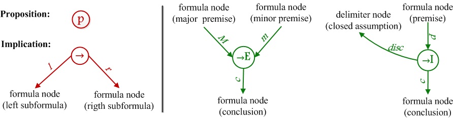
Figure 1: Types of formula nodes of the formula-graph and types of rule nodes of the mimp-graph

The rule nodes, like in Natural Deduction, require the correct number of premises. The premises are indicated by ingoing edges and there are edges from the rule nodes to the conclusion formulas. The right-hand side of Figure 1 shows the rule nodes $\rightarrow$I (implication introduction) and $\rightarrow$E (implication elimination). Note that the discharging of hypotheses may be vacuous. This case in a mimp-graph is represented by a disconnected graph, where the discharged formula node is not linked to the conclusion of the rule by any directed path.

$[p]^{1}$       $p\to q$    $\to$-$E$         $q$        $[q\to r]^{2}$            $\to$-$E$                      $r$                       ($\to$-$I$,1)                    $p\to r$                 ($\to$-$I$,2)              $(q\to r)\to(p\to r)$

$\Downarrow trans$

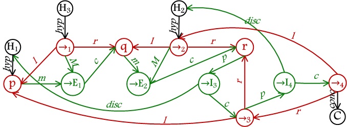
Figure 2: The transition from a natural deduction proof to a mimp-graph

        $[r]^{1}$   $((r\to s)\to r)\to r$      $[(((r\to s)\to r)\to r)\to s]^{3}$                           $s$                          1                       $r\to s$      $[(r\to s)\to r]^{2}$                                                                     $r$                                       2                                    $(((r\to s)\to r)\to r)$      $[(((r\to s)\to r)\to r)\to s]^{3}$                                                                                                        $s$                                                       3                                                    $((((r\to s)\to r)\to r)\to s)\to s$

$\Downarrow trans$

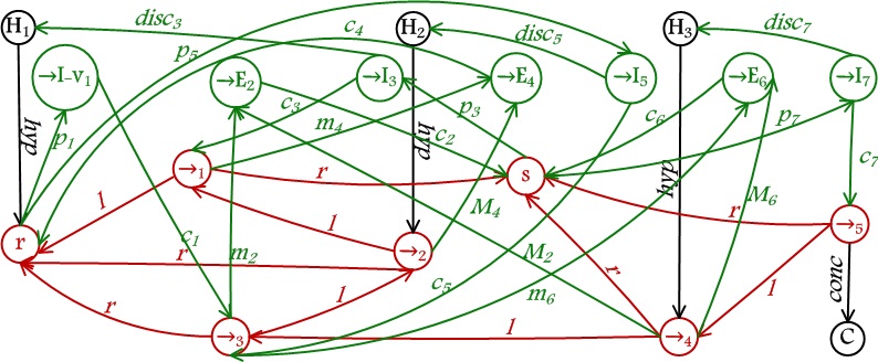
Figure 3: The transition from the derivation of the formula $((((r\to s)\to r)\to r)\to s)\to s$ to a mimp-graph

In the rule nodes, formulas are re-used, which is indicated by putting several arrows towards it, hence the number of ingoing/outgoing edges with label $p$ (premise), $M$ (major premise), $m$ (minor premise) and $c$ (conclusion) coming or going to a formula node could be arbitrarily large. To make all this a bit more intuitive we give an example of a mimp-graph in Figure 2, which can be seen as a derivation of $(q\rightarrow r)\rightarrow(p\rightarrow r)$ from $(p\rightarrow q)$. Indices of discarded hypotheses are replaced by additional edges assigned with the label: $disc$ (discharge). This re-using of formulas is necessary. We remind the reader that some valid implicational formulas, such as $((((r\to s)\to r)\to r)\to s)\to s$ (see Figure 3), need to use twice a subformula in a Natural Deduction proof, in this case the subformula $(((r\to s)\to r)\to r)\to s$ is used twice. Because of this, the edges $p$, $m$, $M$ and $c$ in Figure 3 are indexed in a unique way.

The formula nodes in the graph (Figure 2) are labelled with propositional letters $p$, $q$ and $r$, the connective $\rightarrow$; the rule nodes are labelled with $\rightarrow$E and $\rightarrow$I. The underlying idea is that there is an inferential order between rule nodes that provides the corresponding derivability order; the formula node labelled $\rightarrow_{4}$ linked to the delimiter node $C$ by an edge labelled $conc$ is the root node and the conclusion of the proof represented by the graph. Besides, the node $\rightarrow_{1}$ linked to the delimiter node $H$ by the edge labelled $hyp$ (hypothesis) in the graph is representing the premise $(p\rightarrow q)$.

We want to emphasize that the mimp-graphs put together information on formula-graphs and rule nodes. To make it more transparent we can use bicolored graphs. In this way formula nodes and edges between them are painted red, whereas inference nodes and edges between them and adjacent premises and/or conclusions are painted green. So nodes of types $\to$ and $p$ (propositions) together with adjacent edges $(l,r)$ are red, whereas nodes labelled $\to$I and $\to$E together with adjacent edges $(m,M,p,c,disc)$ are green.

Now we give a formal definition of mimp-graphs.

Definition 1.

L is the union of the four sets of labels types:

• R-Labels is the set of inference labels: {$\to$I${}_{n}/n\in\mathbb{Z}\}\cup\{\to$E${}_{m}/m\in\mathbb{Z}\}$,

• F-Labels is the set of formula labels: {$\to_{i}/i\in\mathbb{N}$} and the propositional letters $\{p,q,r,...\}$,

• E-Labels is the set of edge labels: {$l$ (left), $r$ (right), $conc$ (final conclusion), $hyp$ (hypothesis)$\}$ $\cup$ $\{p_{j}$ (premise)$/j\in\mathbb{Z}\}$ $\cup$ $\{m_{j}$ (minor premise)$/j\in\mathbb{Z}\}$ $\cup$ $\{M_{j}$ (major premise)$/j\in\mathbb{Z}\}$ $\cup$ $\{c_{j}$ (conclusion)$/j\in\mathbb{Z}\}$ $\cup$ $\{disc_{j}$ (discharge)$/j\in\mathbb{Z}\}$,

• D-Labels is the set of delimiter labels: $\{H_{k}/k\in\mathbb{Z}\}\cup\{C\}$.

Definition 2.

A mimp-graph $G$ is a directed graph $\langle$V, E, L, $l_{V}$, $l_{E}\rangle$ where: V is a set of nodes, E is a set of edges, L is a set of labels, $\langle v\in$ V, $t\in$ L, $v^{\prime}\in$ V$\rangle$, where $v$ is the source and $v^{\prime}$ the target, $l_{V}$ is a labeling function from V to R$\cup$F-Labels, $l_{E}$ is a labeling function from E to E-Labels.

Mimp-graphs are defined recursively as follows:

Basis

If $G_{1}$ is a formula graph with root node $\alpha_{m}$ , then the graph $G_{2}$ is defined as $G_{1}$ with the delimiter nodes $H_{n}$ and $C$ and the edges $(\alpha_{m},conc,C)$ and $(H_{n},hyp,\alpha_{m})$ is a mimp-graph.

 $\to$E

If $G_{1}$ and $G_{2}$ are mimp-graphs, and the graph (intermediate step) obtained by $G_{1}\oplus G_{2}$  contains the edge $(\to_{q},l,\alpha_{m})$ and the two nodes $\to_{q}$ and $\alpha_{m}$ linked to the delimiter node $C$, then the graph $G_{3}$ is defined as $G_{1}\oplus G_{2}$ with

1. the removal of the ingoing edges in the node $C$ which were generated in the intermediate step (see Figure 4, dotted area in $G_{1}\oplus G_{2}$);

2. a rule node $\to$E_i at the top level;

3. the edges: $(\alpha_{m},m_{new},\to$E${}_{i})$, $(\to_{q}$, $M_{new}$,$\to$E${}_{i})$, $(\to$E${}_{i},c_{new},\beta_{n})$ and $(\beta_{n},conc,C)$, where $new$ is a fresh (new) index considering all edges of kind $c$, $m$ and $M$ ingoing and/or outgoing the formula-nodes $\alpha_{m}$, $\beta_{n}$ and $\to_{q}$,

is a mimp-graph (see Figure 4).

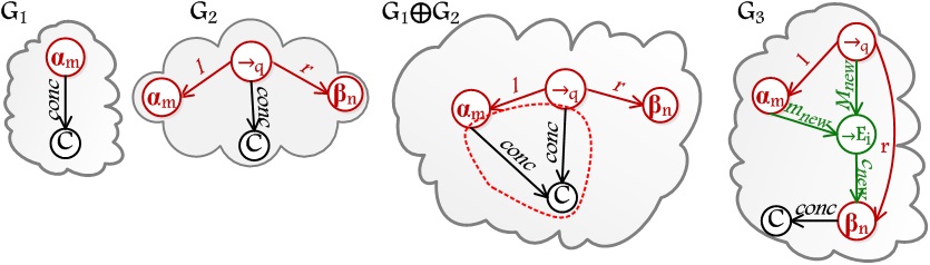
Figure 4: The $\to$E rule of mimp-graph

 $\to$I 

If $G_{1}$ is a mimp-graph and contains a node $\beta_{n}$ linked to the delimiter node $C$ and the node $\alpha_{m}$ linked to the delimiter node $H_{k}$, then the graph $G_{2}$ is defined as $G_{1}$ with

1. the removal of the edges: $(\beta_{n},conc,C)$;

2. a rule node $\to$I_j at the top level;

3. a formula node $\to_{t}$ linked to the delimiter node $C$ by an edge $(\to_{t},conc,C)$;

4. the edges: $(\to_{t},l,\alpha_{m})$, $(\to_{t},r,\beta_{n})$, $(\beta_{n},p_{new},\to$I_j), $(\to$I_j, $c_{new},\to_{t})$, and $(\to$I_j, $disc_{new},H_{k})$, where $new$ is a fresh index concerning ingoing and outgoing edges of type $c$ and $p$ of the formula-nodes $\beta_{n}$, $\to_{t}$ and $\alpha_{m}$,

is a mimp-graph (see Figure 5; the $\alpha_{m}$-node is discharged).

 $\to$I-v

If $G_{1}$ is a mimp-graph, and $G$ is a formula graph with root node $\alpha_{m}$, and $G_{1}$ contains a node $\beta_{n}$ linked to the delimiter node $C$, then the graph $G_{2}$ is defined as $G_{1}\oplus G$ with

1. the removal of the edge: $(\beta_{n},conc,C)$;

2. a rule node $\to$I_j at the top level;

3. a formula node $\to_{t}$ linked to the delimiter node $C$ by an edge $(\to_{t},conc,C)$;

4. the edges: $(\to_{t},l,\alpha_{m})$, $(\to_{t},r,\beta_{n})$, $(\beta_{n},p_{new},\to$I_j) and $(\to$I_j, $c_{new},\to_{t})$, where $new$ is an index under the same conditions of the previous case,

is a mimp-graph (see Figure 6).

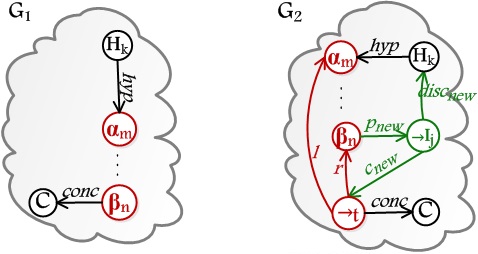
Figure 5: The $\to$I rule of mimp-graph

Figure 6: The $\to$I-v rule of mimp-graph

Lemma1 enables us to prove that a given graph $G$ is a mimp-graph without explicitly supplying a construction. Among others it says that we have to check that each node of $G$ is of one of the possible types that generate the Basis, $\to$E, $\to$I and $\to$I-v construction cases of Definition 2.

Definition 3 (Inferential Ordering).

Let $G$ be a mimp-graph. An inferential order $>$ on nodes of $G$ is a partial ordering of the rule nodes of $G$, such that, $n<n^{\prime}$, iff, $n$ and $n^{\prime}$ are rule nodes, and there is a formula node $f$, such that, n $\xrightarrow{l_{1}}$ f $\xrightarrow{l_{2}}n^{\prime}$ and $l_{1}$ is $c$ and $l_{2}$ is $m$, or , $l_{1}$ is $c$ and $l_{2}$ is $M$, or, $l_{1}$ is $c$ and $l_{2}$ is $p$.

In order to avoid overloading of indexes, we will omit whenever is possible, the indexing of edges of kind $c$, $m$, $M$, $p$ and $disc$, remembering that the coherence of indexing is established by the kind of rule-node to which they are linked.

Lemma 1.

$G$ is a mimp-graph if and only if the following hold:

1. There exists a well-founded (hence acyclic) inferential order $>$ on all rule nodes of the mimp-graph.

2. Every node $N$ of $G$ is of one of the following six types:

   L    

   $N$ is labelled with one of the propositional letters: {p, q, r, … }. $N$ has no outgoing edges $l$ and $r$.

   F    

   $N$ has label $\to_{n}$ and has exactly two outgoing edges with label $l$ and $r$, respectively. $N$ has outgoing edges with labels $p$, $m$ or $M$; and it has at most one ingoing edge with label $c$ and at most one ingoing edge with label $hyp$.

   E    

   $N$ has label $\to$E_i and has exactly one outgoing edge ($\to$E_i, $c$, $\beta_{n}$), where $\beta_{n}$ is a node type L or F. $N$ has exactly two ingoing edges ($\alpha_{m},m,\beta_{n}$) and ($\to_{q},M,\to$E_i), where $\alpha_{m}$ is a node type L or F. There are two outgoing edges from the node $\to_{q}$: $(\to_{q},l,\alpha_{m})$ and $(\to_{q},r,\beta_{n})$.

   I    

   $N$ has label $\to$I_j (or $\to$I-v_j, if discharges an hypothesis vacuously), has one outgoing edge ($\to$I_j, $c$, $\to_{t}$), and one (or zero for the case $\to$I-v) outgoing edge ($\to$I_j, $disc$, $H_{k}$). $N$ has exactly one ingoing edge: $(\beta_{n},p,\to$I${}_{j})$, where $\beta_{n}$ is a node type L or F. There are two outgoing edges from the node $\to_{t}$: $(\to_{t},l,\alpha_{m})$ and $(\to_{t},r,\beta_{n})$.

   H    

   $N$ has label $H_{k}$ and has exactly one outgoing edge $hyp$.

   C    

   $N$ has label C and has exactly one ingoing edge $conc$.

Proof.

$\Rightarrow$: Argue by induction on the construction of mimp-graph (Definition 2). For every construction case for mimp-graphs we have to check the three properties stated in Lemma. Property (2) is immediate. For property (1), we know from the induction hypothesis that there is an inferential order $>$ on rule nodes of the mimp-graph. In the construction cases $\to$I, $\to$I-v or $\to$E, we make the new rule node that is introduced highest in the $>$-ordering, which yields an inferential ordering on rule nodes. In the construction case $\to$E, when we have two inferential orderings, $>_{1}$ on $G_{1}$ and $>_{2}$ on $G_{2}$. Then $G_{1}\oplus G_{2}$ can be given an inferential ordering by taking the union of $>_{1}$ and $>_{2}$ and in addition putting $n>m$ for every rule node $n,m$ such that $n\in G_{1},m\in G_{2}$.

$\Leftarrow$: Argue by induction on the number of rule nodes of $G$. Let $>$ be the topological order that is assumed to exist. Let $n$ be the rule node that is maximal w.r.t. $>$. Then $n$ must be on the top position. When we remove node $n$, including its edges linked (if $n$ is of type I) and the node type $C$ is linked to the premise of the rule node, we obtain a graph $G^{\prime}$ that satisfies the properties listed in Lemma. By induction hypothesis we see that $G^{\prime}$ is a mimp-graph. Now we can add the node $n$ again, using one of the construction cases for mimp-graphs: Basis if $n$ is a L node or F node, $\to$E if $n$ is an E node, $\to$I if $n$ is an I node. ∎

It is natural to consider minimal mimp-graph-like representations of given natural deductions. Actually one can try to minimize the number of F-Labels and/or R-Labels, but for the sake of brevity we consider only the F-option, as it helps to reduce the size under standard normalization (see the next section). To grasp the point note that mimp-graph in Figure 2 (see above) is F-minimal, i.e. its F-labelled nodes refer to pairwise distinct formulas. This observation is summarized by

Theorem 1 (F-minimal representation).

Every standard tree-like natural deduction $\Pi$ has a uniquely determined (up to graph-isomorphism) F-minimal mimp-like representation $G_{\Pi}$, i.e. such a one that satisfies the following four conditions.

1. $G_{\Pi}$ is a mimp-graph whose size does not exceed the size of $\Pi$.

2. $\Pi$ and $G_{\Pi}$ both have the same (set of) hypotheses and the same conclusion.

3. There is graph homomorphism $h:\Pi\rightarrow G_{\Pi}$ that is injective on R-Labels.

4. All F-Labels occurring in $G_{\Pi}$ denote pairwise distinct formulas.

Proof.

Let $N$ and $F$ be the set of nodes and formulas, respectively, occurring in $\Pi$. Note that $\Pi$ determines a fixed surjection $f:N\rightarrow F$ that may not be injective (for in $\Pi$, one and the same formula may be assigned to different nodes). In order to obtain $G_{\Pi}$ take as R-nodes the inferences occurring in $\Pi$ assigned with the corresponding “green” R-Labels representing inferences’ names (possibly indexed, in order to achieve a 1–1 correspondence between inferences and R-Labels, cf. Figure 2). Define basic F-nodes of $G_{\Pi}$ as formulas from $F$ assigned with the corresponding “red” F-Labels representing formulas’ principal connectives (possibly indexed, in order to achieve a 1–1 correspondence between formulas and F-Labels, cf. Figure 2). So the total number of all basic F-nodes of $G_{\Pi}$ is the cardinality of the set $F$, while $f$ being a mapping from the nodes of $\Pi$ onto the basic F-nodes of $G_{\Pi}$. To complete the construction of $G_{\Pi}$ we add, if necessary, the remaining F-nodes labelled by failing “red” representations of subformulas of $f(x)$, $x\in N$, and define the E-Labels of $G_{\Pi}$ (both “green” and “red”), accordingly. Note that by the definition all nodes of $G_{\Pi}$ have pairwise distinct labels. In particular, every F-Label occurs only once in $G_{\Pi}$, which yields the crucial condition 4. ∎

3 Normalization for mimp-graphs

In this section we define the normalization procedure for mimp-graphs. It is based on standard normalization method given by Prawitz. Thus a maximal formula in mimp-graphs is a $\rightarrow$-$I$ followed by a $\rightarrow$-E of the same formula graph (see Definition 4). It is the same notion of maximal formulas that is being used in natural deduction derivations. So a maximal formula occurrence is the consequence of an application of an introduction rule and major premise of an application of an elimination rule. But here we assume that derivations are represented by mimp-graphs. We wish to eliminate such maximal formula by dropping nodes and edges that are involved in the maximal formula. However, it could also happen that between the rule nodes $\rightarrow$-I and $\rightarrow$-E there are several other maximal formulas.

Definition 4.

A maximal formula $m$ in a mimp-graph $G$ (see Figure 7) is a sub-graph of $G$ consisting of:

1. the formula nodes $\alpha_{m}$, $\beta_{n}$, $\to_{q}$, the rule node $\to$I_i and the delimiter node $H_{u}$;

2. the rule node $\to$E_j at the top level;

3. the edges: $(\to_{q},l,\alpha_{m})$, $(\to_{q},r,\beta_{n})$, $(\beta_{n},p,\to$I_i), $(\to$I${}_{i},c,\to_{q})$, $(H_{u},hyp,\alpha_{m})$, $(\to$I${}_{i},disc,H_{u})$, $(\alpha_{m},$ $m,\to$E${}_{j})$, $(\to_{q},M,\to$E${}_{j})$ and $(\to$E${}_{j},c,\beta_{n})$;

$\begin{array}[]{lcr}\ignorespaces\ignorespaces\ignorespaces\ignorespaces\ignorespaces\ignorespaces\ignorespaces\ignorespaces\ignorespaces\ignorespaces\ignorespaces\ignorespaces\ignorespaces\leavevmode\lower 117.07108pt\hbox{\vbox{\vbox{\hbox{\vbox{\hbox{\hskip 4.0pt\hbox{$\Pi_{1}$}\hskip 4.0pt}\vskip 2.0pt\nointerlineskip\hbox{\hskip 0.0pt\lower-0.5pt\hbox{}\hbox{\vbox{\vskip 1.0pt}}\lower-0.5pt\hbox{}}\vskip 2.0pt\nointerlineskip\hbox{\hskip 1.9515pt\hbox{\hbox{\hskip 4.0pt\hbox{$\alpha$}\hskip 4.0pt}}}}\hbox{\hskip 14.45377pt}\vbox{\hbox{\hskip 3.72517pt\vbox{\vbox{\hbox{\hskip 4.0pt\hbox{$[\alpha]^{u}$}\hskip 4.0pt}\vskip 2.0pt\nointerlineskip\hbox{\hskip 0.0pt\lower-0.5pt\hbox{}\hbox{\vbox{\vskip 1.0pt}}\lower-0.5pt\hbox{}}\vskip 2.0pt\nointerlineskip\hbox{\hskip 2.42917pt\hbox{\hbox{\hskip 4.0pt\hbox{$\Pi_{2}$}\hskip 4.0pt}}}}\vskip 2.0pt\nointerlineskip\hbox{\hskip 2.42917pt\lower-0.5pt\hbox{}\hbox{\vbox{\vskip 1.0pt}}\lower-0.5pt\hbox{}}\vskip 2.0pt\nointerlineskip\hbox{\hskip 4.75105pt\hbox{\hbox{\hskip 4.0pt\hbox{$\beta$}\hskip 4.0pt}}}}}\vskip 0.04723pt\nointerlineskip\hbox{\hskip 0.0pt\lower-0.2pt\hbox{}\hbox to30.6087pt{\xleaders\hrule\hfill}\lower 1.95277pt\hbox{\hskip 3.0pt$u$}}\vskip 0.04723pt\nointerlineskip\hbox{\hbox{\hskip 4.0pt\hbox{$\alpha\to\beta$}\hskip 4.0pt}}}}\vskip 2.0pt\nointerlineskip\hbox{\hskip 1.9515pt\lower-0.2pt\hbox{}\hbox to61.41098pt{\xleaders\hrule\hfill}\lower-0.2pt\hbox{}}\vskip 2.0pt\nointerlineskip\hbox{\hskip 25.82887pt\hbox{\hbox{\hskip 4.0pt\hbox{$\beta$}\hskip 4.0pt}}}}\vskip 2.0pt\nointerlineskip\hbox{\hskip 23.50699pt\lower-0.5pt\hbox{}\hbox{\vbox{\vskip 1.0pt}}\lower-0.5pt\hbox{}}\vskip 2.0pt\nointerlineskip\hbox{\hskip 23.50699pt\hbox{\hbox{\hskip 4.0pt\hbox{$\Pi_{3}$}\hskip 4.0pt}}}}}\ignorespaces\hskip 28.45274pt\Rightarrow\par\par\end{array}$

Figure 7: Maximal formula in mimp-graphs

Definition 5.

(1) For $n_{i}\in V$, a p-path in a proof-graph is a sequence of vertices and edges of the form: $n_{1}\xrightarrow{l_{1}}n_{2}\xrightarrow{l_{2}}...\xrightarrow{l_{k-2}}n_{k-1}\xrightarrow{l_{k-1}}n_{k}$, such that $n_{1}$ is a hypothesis formula node, $n_{k}$ is the conclusion formula node, $n_{i}$ alternating between a rule node and a formula node. The edges $l_{i}$ alternate between two types of edges: the first is $l_{j}\in\{m,M,p\}$ and the second $l_{j}=c$. (2) A  branch is an initial part of a p-path which stops at the conclusion formula node or at the first minor premise whose major premise is the conclusion of a rule node.

Definition 6.

Let $G$ a graph obtained by dropping rule nodes in a mimp-graph then, the reordering of $G$ is defined as the graph $G$ with the following (new) inference order on the rule nodes of $G$.

• $o(t_{m})=0$ for a rule node $t_{m}$ starting with hypothesis.

• $o(t)=o(t^{\prime})+1$ if the conclusion formula of rule node $t^{\prime}$ is premise or major premise of $t$.

Proposition 1.

If a graph $G$ is obtained by a reordering by means of the operation defined in Definition 6 then, $G$ is a mimp-graph.

Definition 7.

Given a mimp-graph $G$ with a maximal formula $m$, eliminating a maximal formula is the following transformation of a mimp-graph, where the maximal formula $m$ satisfies the following requirements:

1. Between the rule nodes $\to$I_i and $\to$E_l there are zero or more maximal formulas with inferential orders within the range of these rule nodes.

2. There is an edge $(\to$I${}_{i},c,\to_{q})$, and, the formula node $\to_{q}$ has zero or more ingoing edges.

3. There is an edge $(\to_{q},M,\to$E${}_{l})$, and, the formula node $\to_{q}$ is the premise of zero or more of another rule nodes.

4. If a branch will be separated from the inferential order this branch must be insertable in the following branch, according to the order, i.e. the conclusion of this separated branch is the premise in the following branch.

The elimination of a maximal formula is the following operation on a mimp-graph (see Figure 8, the dotted arrows are representing sets of edges):

1. If there is no maximal formula between the rule nodes $\rightarrow$I_i and $\rightarrow$E_l then follow these steps:

   1. If the edge $(\to$I${}_{i},c,\to_{q})$ is the only ingoing edge to $\to_{q}$ and the edge $(\to_{q},M,\to$E${}_{l})$ is the only outgoing edge from $\to_{q}$ then remove the edges to and from the formula node $\to_{q}$, and the formula node $\to_{q}$.

   2. Remove the edges to and from the nodes $\to$I_i, $\to$E_l and $H_{u}$.

   3. Remove the nodes $\to$I_i, $\to$E_l and $H_{u}$.

   4. Apply the operation defined in Definition 6 to the resulting graph. Note that Proposition 1 ensures that the result is a mimp-graph.

2. Otherwise eliminate the maximal formulas between the rule nodes $\to$I_i and $\to$E_l as in the previous step.

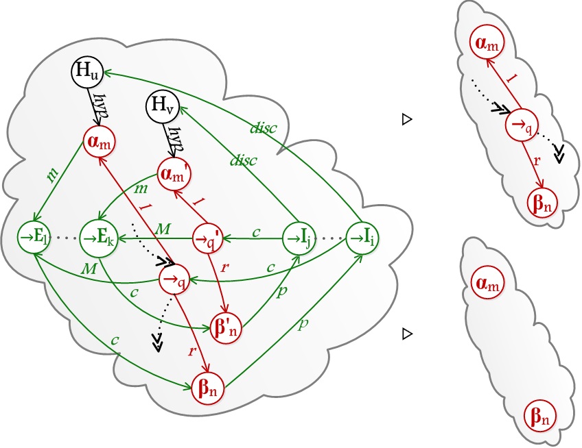
Figure 8: Elimination of a maximal formula in mimp-graphs

Note that the removal of a node $\to$I generated by case $\to$I-v, in the Definition 2, disconnects the graph meaning that the sub-graph hypotheses linked, by the edge $m$, to eliminated node $\to$-E is no longer connected to the delimiter $C$.

$\begin{array}[]{lcr}\ignorespaces\ignorespaces\ignorespaces\par\ignorespaces\ignorespaces\ignorespaces\par\ignorespaces\ignorespaces\ignorespaces\ignorespaces\ignorespaces\ignorespaces\ignorespaces\ignorespaces\ignorespaces\par\ignorespaces\par\ignorespaces\leavevmode\lower 135.69196pt\hbox{\vbox{\hbox{\vbox{\hbox{\hskip 4.0pt\hbox{$\Pi_{2}$}\hskip 4.0pt}\vskip 2.0pt\nointerlineskip\hbox{\hskip 0.0pt\lower-0.5pt\hbox{}\hbox{\vbox{\vskip 1.0pt}}\lower-0.5pt\hbox{}}\vskip 2.0pt\nointerlineskip\hbox{\hskip 2.0897pt\hbox{\hbox{\hskip 4.0pt\hbox{$\beta$}\hskip 4.0pt}}}}\hbox{\hskip 14.45377pt}\vbox{\hbox{\vbox{\hbox{\hskip 4.0pt\hbox{$\Pi_{1}$}\hskip 4.0pt}\vskip 2.0pt\nointerlineskip\hbox{\hskip 0.0pt\lower-0.5pt\hbox{}\hbox{\vbox{\vskip 1.0pt}}\lower-0.5pt\hbox{}}\vskip 2.0pt\nointerlineskip\hbox{\hskip 1.75636pt\hbox{\hbox{\hskip 4.0pt\hbox{$\alpha$}\hskip 4.0pt}}}}\hbox{\hskip 14.45377pt}\vbox{\hbox{\hskip 7.5753pt\vbox{\vbox{\vbox{\hbox{\hskip 4.0pt\hbox{$[\beta]^{v}[\alpha]^{u}$}\hskip 4.0pt}\vskip 2.0pt\nointerlineskip\hbox{\hskip 0.0pt\lower-0.5pt\hbox{}\hbox{\vbox{\vskip 1.0pt}}\lower-0.5pt\hbox{}}\vskip 2.0pt\nointerlineskip\hbox{\hskip 8.54346pt\hbox{\hbox{\hskip 4.0pt\hbox{$\Pi_{0}$}\hskip 4.0pt}}}}\vskip 2.0pt\nointerlineskip\hbox{\hskip 8.54346pt\lower-0.5pt\hbox{}\hbox{\vbox{\vskip 1.0pt}}\lower-0.5pt\hbox{}}\vskip 2.0pt\nointerlineskip\hbox{\hskip 10.84868pt\hbox{\hbox{\hskip 4.0pt\hbox{$\gamma$}\hskip 4.0pt}}}}\vskip 0.2625pt\nointerlineskip\hbox{\hskip 3.55336pt\lower-0.2pt\hbox{}\hbox to27.25021pt{\xleaders\hrule\hfill}\lower 1.73749pt\hbox{\hskip 3.0pt$v$}}\vskip 0.26251pt\nointerlineskip\hbox{\hskip 3.55336pt\hbox{\hbox{\hskip 4.0pt\hbox{$\beta\to\gamma$}\hskip 4.0pt}}}}}\vskip 0.2625pt\nointerlineskip\hbox{\hskip 0.0pt\lower-0.2pt\hbox{}\hbox to49.50754pt{\xleaders\hrule\hfill}\lower 1.73749pt\hbox{\hskip 3.0pt$u$}}\vskip 0.26251pt\nointerlineskip\hbox{\hbox{\hskip 4.0pt\hbox{$\alpha\to(\beta\to\gamma)$}\hskip 4.0pt}}}}\vskip 2.0pt\nointerlineskip\hbox{\hskip 1.75636pt\lower-0.2pt\hbox{}\hbox to79.47496pt{\xleaders\hrule\hfill}\lower-0.2pt\hbox{}}\vskip 2.0pt\nointerlineskip\hbox{\hskip 27.86873pt\hbox{\hbox{\hskip 4.0pt\hbox{$\beta\to\gamma$}\hskip 4.0pt}}}}}\vskip 2.0pt\nointerlineskip\hbox{\hskip 2.0897pt\lower-0.2pt\hbox{}\hbox to84.75302pt{\xleaders\hrule\hfill}\lower-0.2pt\hbox{}}\vskip 2.0pt\nointerlineskip\hbox{\hskip 38.13643pt\hbox{\hbox{\hskip 4.0pt\hbox{$\gamma$}\hskip 4.0pt}}}}}\ignorespaces&\hfil\rhd\hskip 14.22636pt\ignorespaces\ignorespaces\ignorespaces\ignorespaces\ignorespaces\ignorespaces\ignorespaces\ignorespaces\ignorespaces\ignorespaces\ignorespaces\ignorespaces\ignorespaces\leavevmode\lower 111.66446pt\hbox{\vbox{\hbox{\vbox{\hbox{\hskip 4.0pt\hbox{$\Pi_{2}$}\hskip 4.0pt}\vskip 2.0pt\nointerlineskip\hbox{\hskip 0.0pt\lower-0.5pt\hbox{}\hbox{\vbox{\vskip 1.0pt}}\lower-0.5pt\hbox{}}\vskip 2.0pt\nointerlineskip\hbox{\hskip 2.0897pt\hbox{\hbox{\hskip 4.0pt\hbox{$\beta$}\hskip 4.0pt}}}}\hbox{\hskip 14.45377pt}\vbox{\vbox{\vbox{\hbox{\hbox{\hskip 4.0pt\hbox{$[\beta]^{v}$}\hskip 4.0pt}\hbox{\hskip 14.45377pt}\vbox{\hbox{\hskip 4.0pt\hbox{$\Pi_{1}$}\hskip 4.0pt}\vskip 2.0pt\nointerlineskip\hbox{\hskip 0.0pt\lower-0.5pt\hbox{}\hbox{\vbox{\vskip 1.0pt}}\lower-0.5pt\hbox{}}\vskip 2.0pt\nointerlineskip\hbox{\hskip 1.75636pt\hbox{\hbox{\hskip 4.0pt\hbox{$\alpha$}\hskip 4.0pt}}}}}\vskip 2.0pt\nointerlineskip\hbox{\hskip 0.0pt\lower-0.5pt\hbox{}\hbox{\vbox{\vskip 1.0pt}}\lower-0.5pt\hbox{}}\vskip 2.0pt\nointerlineskip\hbox{\hskip 16.70593pt\hbox{\hbox{\hskip 4.0pt\hbox{$\Pi_{0}$}\hskip 4.0pt}}}}\vskip 2.0pt\nointerlineskip\hbox{\hskip 16.70593pt\lower-0.5pt\hbox{}\hbox{\vbox{\vskip 1.0pt}}\lower-0.5pt\hbox{}}\vskip 2.0pt\nointerlineskip\hbox{\hskip 19.01115pt\hbox{\hbox{\hskip 4.0pt\hbox{$\gamma$}\hskip 4.0pt}}}}\vskip 2.0pt\nointerlineskip\hbox{\hskip 11.71584pt\lower-0.2pt\hbox{}\hbox to27.25021pt{\xleaders\hrule\hfill}\lower-0.2pt\hbox{}}\vskip 2.0pt\nointerlineskip\hbox{\hskip 11.71584pt\hbox{\hbox{\hskip 4.0pt\hbox{$\beta\to\gamma$}\hskip 4.0pt}}}}}\vskip 2.0pt\nointerlineskip\hbox{\hskip 2.0897pt\lower-0.2pt\hbox{}\hbox to68.60013pt{\xleaders\hrule\hfill}\lower-0.2pt\hbox{}}\vskip 2.0pt\nointerlineskip\hbox{\hskip 30.05998pt\hbox{\hbox{\hskip 4.0pt\hbox{$\gamma$}\hskip 4.0pt}}}}}\ignorespaces\hskip 14.22636pt\rhd&\ignorespaces\ignorespaces\ignorespaces\ignorespaces\ignorespaces\ignorespaces\ignorespaces\leavevmode\lower 68.69948pt\hbox{\vbox{\vbox{\vbox{\hbox{\hskip 2.90395pt\hbox{\hskip 4.0pt\hbox{$\Pi_{2}$ \ $\Pi_{1}$}\hskip 4.0pt}}\vskip 2.0pt\nointerlineskip\hbox{\hskip 0.0pt\lower-0.5pt\hbox{}\hbox{\vbox{\vskip 1.0pt}}\lower-0.5pt\hbox{}}\vskip 2.0pt\nointerlineskip\hbox{\hbox{\hskip 4.0pt\hbox{$\beta$ \ \ \ \ $\alpha$}\hskip 4.0pt}}}\vskip 2.0pt\nointerlineskip\hbox{\hskip 0.0pt\lower-0.5pt\hbox{}\hbox{\vbox{\vskip 1.0pt}}\lower-0.5pt\hbox{}}\vskip 2.0pt\nointerlineskip\hbox{\hskip 11.28896pt\hbox{\hbox{\hskip 4.0pt\hbox{$\Pi_{0}$}\hskip 4.0pt}}}}\vskip 2.0pt\nointerlineskip\hbox{\hskip 11.28896pt\lower-0.5pt\hbox{}\hbox{\vbox{\vskip 1.0pt}}\lower-0.5pt\hbox{}}\vskip 2.0pt\nointerlineskip\hbox{\hskip 13.59418pt\hbox{\hbox{\hskip 4.0pt\hbox{$\gamma$}\hskip 4.0pt}}}}}\par\ignorespaces\end{array}$

$\Downarrow trans$

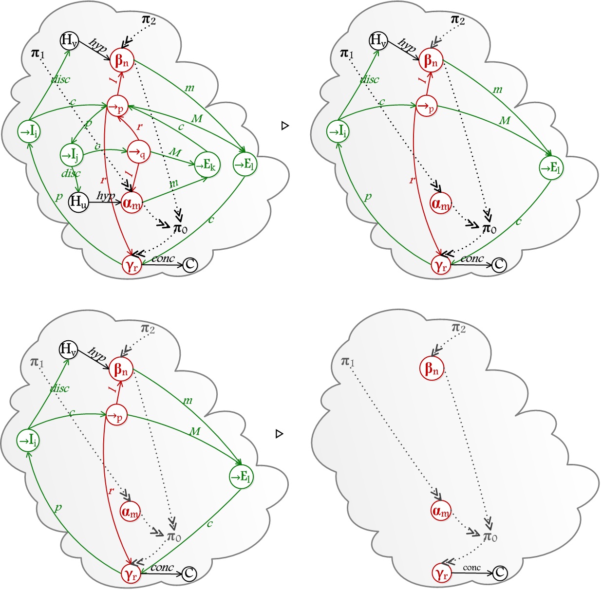
Figure 9: Eliminating a maximal formula in a natural deduction proof and its mimp-graph translation

Let us show in Figure 9 an instance of the eliminating a maximal formula in tree form. Note that this example shows the reason why essentially our (weak) normalization theorem is directly a strong normalization theorem. The formula $\beta\to\gamma$ is not a maximal formula before a reduction is applied to eliminate the maximal formula $\alpha\to(\beta\to\gamma)$. This possibility of having hidden maximal formulas in Natural Deduction is the main reason to use more sophisticated methods whenever proving strong normalization. In mimp-graphs there is no possibility to hide a maximal formula because all formulas are represented only once in the graph. In this graph $\beta\to\gamma$ is already a maximal formula. We can choose to remove any of the two maximal formulas. If $\beta\to\gamma$ is chosen to be eliminated, by the mimp-graph normalization procedure, its reduction eliminates the $\alpha\to(\beta\to\gamma)$ too. On the other hand, the choice of $\alpha\to(\beta\to\gamma)$ to be reduced only eliminates itself. In any case the number of maximal formula decreases.

We shall construct the normalization proof for mimp-graphs. This proof is guided by the normalization measure. That is, the general mechanism from the proof determines that a given mimp-graph $G$ should be transformed into a non-redundant mimp-graph by applying of reduction steps and at each reduction step the measure must be decreased. The normalization measure will be the number of maximal formulas in the mimp-graph.

Also note a following important observation concerning F-minimal mimp representations (see Theorem 1). Since F-minimal mimps can have at most one occurrence of hypotheses $\alpha$ and/or $\beta$, every proper reduction step will diminish the size of deduction. Hence the size of the graph (= the number of nodes) can serve as another inductive parameter, provided that the normalization is being applied to F-minimal mimp-graph representations.

Theorem 2 (Normalization).

Every mimp-graph $G$ can be reduced to a normal mimp-graph $G^{\prime}$ having the same hypotheses and conclusion as $G$. Moreover, for any standard tree-like natural deduction $\Pi$, if $G:=G_{\Pi}$ (the F-minimal mimp-like representation of $\Pi$, cf. Theorem 1), then the size of $G^{\prime}$ does not exceed the size of $G$, and hence also $\Pi$.

Remark 3.

The second assertion sharply contrasts to the well-known exponential speed-up of standard normalization. Note that the latter is a consequence of the tree-like structure of standard deductions having different occurrences of equal hypotheses formulas, whereas all formulas occurring in F-minimal mimp-like representations are pairwise distinct.

Proof.

This characteristic of preservation of the premises and conclusions of the derivation is proved naturally. Through an inspection of each elimination of maximal formula is observed that the reduction step (see Definition 7) of the mimp-graph does not change the set of premises and conclusions (indicated by the delimiter nodes $H$ and $C$) of the derivation that is being reduced.

In addition, the demonstration of this theorem has two primary requirements. First, we guarantee that through the elimination of maximal formulas in the mimp-graph, cannot generate more maximal formulas.The second requirement is to guarantee that during the normalization process, the normalization measure adopted is always reduced.

The first requirement is easily verifiable through an inspection of each case in the elimination of maximal formulas. Thus, it is observed that no case produces more maximal formulas. The second requirement is established through the normalization procedure and demonstrated through an analysis of existing cases in the elimination of maximal formulas in mimp-graphs. To support this statement, it is used the notion of normalization measure, we adopt as measure of complexity (induction parameter) the number of maximal formulas $Nmax(G)$. Besides, as already mentioned, working with F-mimimal mimp-graph representations we can use as optional inductive parameter the ordinary size of mimp-graphs. ∎

Normalization Process

We know that a specific mimp-graph $G$ can have one or more maximal formulas represented by $M_{1},...,M_{n}$. Thus, the normalization procedure is described by the following steps:

1. Choosing a maximal formula represented by $M_{k}$.

2. Identify the respective number of maximal formulas $Nmax(G)$.

3. Eliminate maximal formula $M_{k}$ as defined in Definition 7.

4. In this application one of the following three cases may occur:

   a)

   The maximal formula is removed.

   b)

   The maximal formula is removed but the formula node is maintained, hence $Nmax(G)$ is decreased;

   c)

   All maximal formulas are removed.

5. We repeat this process until the normalization measure $Nmax$ is reduced to zero and $G$ becomes a normal mimp-graph.

Since the process of the eliminating a maximal formula on mimp-graphs always ends in the elimination of at least one maximal formula, and with the decrease in the number of vertices of the graph, we can say that this normalization theorem is directly a strong normalization theorem.

4 Conclusions and Related works

This representation of a proof in mimp-graph requires fewer nodes than the tree and the list representation of proofs. For the case of lists, it is enough to observe that a sub-formula of a formula is already in any graph representation of it. If both take part in the proof the size is smaller than in the mentioned representations. The ability to represent any Natural Deduction proof is preserved. Another important advantage of a compact representation of graphs is that it allows to deduce some structural properties of proof-graphs, for example based on a mimp-graph, it is easy to see an upper bound in the length of the reduction sequence to obtain a normal proof. It is the number of maximal formulas.

There is some previous research concerning the use of graphs to represent proofs developed on connections to substructural logics as Linear Logic, see [8] and [7] for example. The main motivation of this just mentioned investigations is to provide a sound way of representing Linear Logic proofs without dealing with unique labeling and complicated rules for relabeling and discharging mechanisms need to represent Linear Logic proofs as trees in Natural Deduction styles as well as in Sequent Calculus. Proof-nets were such representations and a syntactical criteria on the possible paths on them were considered as a soundness criteria for a proof-graph to be a proof-net. Proof-nets have a cut-rule quite similar to the cut in Sequent Calculus. For the Multiplicative fragment of Classical Linear Logic, there is a linear time cut-elimination theorem. However, when the additive versions of the connectives are considered, the usual complexity of the cut-elimination raises up again. Linear Logic is an important Logic whenever we consider the study of a concurrent computational systems and its semantics strongly uses concurrency theory concepts. Our investigations, on the other hand, is not motivated by proof-theoretical semantics . From the purely proof-theoretical point of view, we use graphs to reduce the redundancy in proofs in such a way that we do not allow hidden maximal formulas in our graph representation of a Natural Deduction proof. As a secondary motivation, this is a preliminary step into investigating how a theorem prover based on graphs is more efficient than usual theorem provers. Our proof-graphs represent the formulas themselves in a way that each subformula is a unique node in the graph. Proof nets do not represent formulas in this way.

References

- [1]
- [2] Sandra Alves, Maribel Fernández & Ian Mackie (2011): A new graphical calculus of proofs. In Rachid Echahed, editor: Proceedings of TERMGRAPH 2011, EPTCS 48, pp. 69–84, 10.4204/EPTCS.48.8.
- [3] Maria Luisa Bonet & Samuel R. Buss (1993): The Deduction Rule and Linear and Near-Linear Proof Simulations. Journal of Symbolic Logic 58(2), pp. 688–709, 10.2307/2275228.
- [4] Vaston Gonçalves da Costa (2007): Compactação de Provas Lógicas. Ph.D. thesis, Departamento de Informática, PUC–Rio. Available at http://www.maxwell.lambda.ele.puc-rio.br/Busca_etds.php?strSecao=resultado&nrSeq=10018@2.
- [5] M. Finger (2005): DAG Sequent Proofs with a Substitution Rule. In: We will show Them – Essays in honour of Dov Gabbay 60th birthday, Kings College Publications 1, Kings College, London, pp. 671–686. Available at http://www.ime.usp.br/~mfinger/home/papers/FW04.pdf.
- [6] Herman Geuvers & Iris Loeb (2007): Natural Deduction via Graphs: Formal Definition and Computation Rules. Mathematical. Structures in Comp. Sci. 17(3), pp. 485–526, 10.1017/S0960129507006123.
- [7] J.-Y. Girard, Y. Lafont & L. Regnier (1995): Advances in Linear Logic. Cambridge University Press, 10.1017/CBO9780511629150. Proceedings of the Workshop on Linear Logic, Ithaca, New York, June 1993.
- [8] Jean yves Girard (1996): Proof-nets: The parallel syntax for proof-theory. In: Logic and Algebra, Dekker, pp. 97–124. Available at iml.univ-mrs.fr/~girard/Proofnets.ps.gz.
- [9] L. Gordeev, E. H. Haeusler & V. G. Costa (2009): Proof compressions with circuit-structured substitutions. Journal of Mathematical Sciences 158(5), pp. 645–658, 10.1007/s10958-009-9405-3.
- [10] E.H. Haeusler (2013): A proof-theoretical discussion on the mechanization of propositional logics. Electronic Proceedings in Theoretical Computer Science Vol. 113, pp. 7-8, 10.4204/EPTCS.113. Available at http://rvg.web.cse.unsw.edu.au/eptcs/content.cgi?LSFA2012#EPTCS113.3.
- [11] Anjolina Grisi Oliveira & Ruy J.G.B. Queiroz (2003): Geometry of Deduction Via Graphs of Proofs. In Ruy J.G.B. Queiroz, editor: Logic for Concurrency and Synchronisation, Trends in Logic 15, Springer Netherlands, pp. 3–88, 10.1007/0-306-48088-3_1.
- [12] R. Statman (1979): Intuitionistic Propositional Logic is Polynomial-Space Complete. Theoretical Computer Science 9, pp. 67–72, 10.1016/0304-3975(79)90006-9. Available at http://www.sciencedirect.com/science/article/pii/0304397579900069.