Towards a GPU-based implementation of interaction nets

Abstract

We present ingpu, a GPU-based evaluator for interaction nets that heavily utilizes their potential for parallel evaluation. We discuss advantages and challenges of the ongoing implementation of ingpu and compare its performance to existing interaction nets evaluators.

1 Introduction

Interaction nets are a model of computation based on graph rewriting. They enjoy several useful properties which makes them a promising candidate for a future functional programming language. In particular, reducible expressions in a net can be evaluated in any order, even in parallel. This makes an implementation of interaction nets on a multicore architecture attractive.

However, the amount of parallelism in an interaction net is highly dynamic, and depends on the particular program and even runtime values. At any point during a computation, the number of expressions that can be evaluated in parallel can vary between dozens and hundreds of thousands. There is currently no implementation of interaction nets that leverages their full parallelism potential.

In recent years, a trend towards using graphics processing units (GPUs) for general purpose computations has emerged. Due to the increasing programability of GPUs and general purpose APIs (CUDA, OpenCL), the parallel processing power of graphics cards may be used for many kinds of problems, from simulation of physical phenomena to cracking passwords. In this paper, we investigate the parallel evaluation of interaction nets using GPUs. While the GPU model of parallelism seems to fit interaction nets well, several factors make an implementation a non-trivial task. We argue that these factors can be overcome, thus enabling an efficient evaluation of interaction nets. Furthermore, we describe our ongoing prototype implementation. Our contributions can be summarized as follows:

• We describe ingpu, the first interaction nets evaluator that runs almost entirely on the GPU, and heavily utilizes their potential for parallel evaluation.

• We describe the underlying algorithm and show its correctness.

• We present benchmark results of the ongoing implementation, and discuss possible solutions to overcome current performance drawbacks.

In the next section, we recall the main notions of interaction nets and the lightweight calculus, which is the basis for our implementation. Section 3 describes the current status of our prototype implementation using the CUDA Thrust library. We follow this description with benchmark results and discuss possible performance improvements in Section 4. Finally, we discuss related work and conclude in Section 5.

2 Preliminaries

2.1 Interaction nets

We now recap the main notions of interaction nets and the lightweight interaction calculus. Interaction nets were first introduced in [10]. A net is a graph consisting of agents (labeled nodes) and ports (edges). Every agent has exactly one principal port (denoted by an arrow), all other ports are called auxiliary ports. The number of auxiliary ports is the arity of the agent. Agent labels denote data or function symbols, and are assigned a fixed arity. Computation is modeled by rewriting the graph, which is based on interaction rules. These rules apply to two nodes which are connected by their principal ports (indicated by the arrows), forming an active pair (or redex). For example, the following rules model the addition of natural numbers (encoded by 0 and a successor function $S$):

This simple system allows for parallel evaluation of programs because by definition active pairs are completely independent. Reducing a pair cannot change, destroy or duplicate another one. Furthermore, any order of evaluation yields the same result. Active pairs may even be reduced in parallel. This is due to the following property.

Proposition 2.1.1 (Uniform Confluence [10]).

Let $P$ be an interaction net, and $\Rightarrow$ the reduction relation induced by a set of rules $R$. Then the following holds: if $N\Rightarrow P$ and $N\Rightarrow Q$ where $P\neq Q$, then there exists some $R$ such that $P\Rightarrow R\Leftarrow Q$.

Example 2.1.2.

Consider the interaction rules for addition of natural numbers. We can model the evaluation of the term $1+(0+1)$ with the following reduction in interaction nets (the active pair evaluated in each step is bold):

After three steps, we reach the expected result $S(S(0))$, corresponding to $2$. Note that each step only reduces one active pair. However, the third step (reduction of $+$ and $0$) could be applied in parallel with either step one or two, yielding the same result.

Remark

This example illustrates the dynamics of the parallelism of interaction nets: depending on the state of the computation, one or two active pairs exist at the same time, and can hence be evaluated in parallel. For particular sets of rules and input nets, the number of concurrent active pairs can get as high as hundreds of thousands. On the other hand, some interaction nets may be inherently sequential.

2.2 The lightweight calculus

The lightweight calculus [6] is a textual representation of interaction nets, providing the basis for our implementation. It handles application of rules as well as rewiring and connecting of ports and agents. It uses the following ingredients:

Symbols $\Sigma$

representing agents, denoted by $\alpha,\beta,\gamma$.

Names $\mathrm{N}$

representing ports, denoted by $x,y,z,x_{1},y_{1},z_{1},\ldots$ . We denote sequences of names by $\overline{x},\overline{y},\overline{z}$.

Terms $\mathrm{T}$

being either names or symbols with a number of subterms, corresponding to the agent’s arity: $t=x\;|\;\alpha(t_{1},\ldots,t_{n})$ . Terms are denoted by $s,t,u$, while $\overline{s},\overline{t},\overline{u}$ denote sequences of terms.

Equations $E$

denoted by $t=s$ where $t,s$ are terms, representing connections in a net. Note that $t=s$ is equivalent to $s=t$. We use $\Delta,\Theta$ to denote multisets of equations.

Configurations $C$

representing a net by $\langle\overline{t}\;|\;\Delta\rangle$. $\overline{t}$ is the interface of the net, i.e., its ports that are not connected to an agent. All names in a configuration occur at most twice. Names that occur twice are called bound.

Interaction Rules $\mathrm{R}$

denoted by $\alpha(\overline{x})=\beta(\overline{y})\longrightarrow\Theta$. $\alpha,\beta$ is the active pair of the left-hand side (LHS) of the rule and the set of equations $\Theta$ represents the right-hand side (RHS).

Rewriting a net is modeled by applying four reduction rules to a configuration:

Communication:

$\langle\;\bar{t}\;|\;x=t,x=u,\Delta\rangle\stackrel{{\scriptstyle com}}{{\longrightarrow}}\ \langle\;\bar{t}\;|\;t=u,\Delta\rangle$

Substitution:

$\langle\;\bar{t}\;|\;x=t,u=s,\Delta\rangle\stackrel{{\scriptstyle sub}}{{\longrightarrow}}\ \langle\;\bar{t}\;|\;u[t/x]=s,\Delta\rangle$, where $u$ is not a variable.

Collect

$\langle\;\bar{t}\;|\;x=t,\Delta\rangle\stackrel{{\scriptstyle col}}{{\longrightarrow}}\ \langle\;\bar{t}[t/x]\;|\;\Delta\rangle$, where $x$ occurs in $\bar{t}$.

Interaction

$\langle\;\bar{t}\;|\;\alpha(\bar{t_{1}})=\beta(\bar{t_{2}}),\Delta\rangle\stackrel{{\scriptstyle int}}{{\longrightarrow}}\langle\;\bar{t}\;|\;\Theta^{\prime},\Delta\rangle$, where $\alpha(\bar{s_{1}})=\beta(\bar{u_{2}})\rightarrow\Theta\;\in\mathrm{R}$. $\Theta^{\prime}$ denotes $\Theta$ where all bound variables in $\Theta$ are replaced by fresh variables and $\bar{s},\bar{u}$ are replaced by $\bar{t_{1}},\bar{t_{2}}$.

Intuitively, $\;\stackrel{{\scriptstyle int}}{{\longrightarrow}}\;$replaces an active pair by the RHS of the corresponding rule. The other three reduction rules substitute variables, which corresponds to resolving a connection between two agents.

Example 1.

The rules for addition presented in Section 2.1 are expressed in the lightweight calculus as follows:

$$+(y,r)=S(x) \;\;\longrightarrow\;\;+(y,w)=x,\;r=S(w)$$ (1)

$$+(y,r)=Z \;\;\longrightarrow\;\;r=y$$ (2)

The following reduction calculates $1+0$:

$$\langle\;r\;|\;+(r,0)=S(0)\;\rangle \stackrel{{\scriptstyle int}}{{\longrightarrow}} \langle\;r\;|\;r=S(x),+(x,0)=0\;\rangle \stackrel{{\scriptstyle col}}{{\longrightarrow}} \langle\;S(x)\;|\;+(x,0)=0\;\rangle$$

$$\stackrel{{\scriptstyle int}}{{\longrightarrow}} \langle\;S(x)\;|\;x=0\;\rangle \stackrel{{\scriptstyle col}}{{\longrightarrow}} \langle\;S(0)\;|\;\;\rangle$$

It is important to note that substitutions done by $\;\stackrel{{\scriptstyle sub}}{{\longrightarrow}}\;$and $\;\stackrel{{\scriptstyle col}}{{\longrightarrow}}\;$never yield a new active pair/equation. This means that we can reach a normal form of a net (i.e., free of active pairs) by using only $\;\stackrel{{\scriptstyle int}}{{\longrightarrow}}\;$and $\;\stackrel{{\scriptstyle com}}{{\longrightarrow}}\;$rules:

Theorem 1 ([6]).

If $C_{1}\longrightarrow^{*}C_{2}$ then there is a configuration $C$ such that $C_{1}\longrightarrow^{*}C\stackrel{{\scriptstyle sub}}{{\longrightarrow}}^{*}.\stackrel{{\scriptstyle col}}{{\longrightarrow}}^{*}C_{2}$, and $C_{1}$ is reduced to $C$ applying only communication and interaction rules.

This theorem can be interpreted as follows. In the lightweight calculus, the lion’s share of the computation is done by $\;\stackrel{{\scriptstyle int}}{{\longrightarrow}}\;$and $\;\stackrel{{\scriptstyle com}}{{\longrightarrow}}\;$. The former reduces expressions (i.e., equations/active pairs) by replacing them with the RHS of the corresponding interaction rule. The latter generates new active equations that can be reduced by $\;\stackrel{{\scriptstyle int}}{{\longrightarrow}}\;$. The collect and substitution steps are in a sense cosmetic: both resolve variables in order to provide a better readable form of the result net. They perform no “actual” computation, i.e., rewriting of the graph represented by the set of equations. Hence, all $\;\stackrel{{\scriptstyle sub}}{{\longrightarrow}}\;$and $\;\stackrel{{\scriptstyle col}}{{\longrightarrow}}\;$steps can be pushed to the end of the computation.

3 Parallel evaluation of interaction nets in CUDA/Thrust

In this section, we discuss the ongoing implementation of our GPU-based interaction nets evaluator ingpu. First, we give a quick introduction to CUDA/Thrust and motivate a GPU-based approach. We then describe the main components of the evaluator, the interaction and the communication phase.

3.1 CUDA and Thrust

The tool ingpu is written in C++ and CUDA. The latter is a language for GPU-based, general-purpose computation on NVIDIA graphics cards. The general flow of a program using the GPU for data-parallel computation is as follows: an array of input data sets is copied from the main memory (known as host memory) to the memory of the GPU (also referred to as device). A function (the kernel) is executed on the GPU in parallel on each individual data set. Finally, the array of results is copied back to main memory.

In general, implementing an algorithm on a GPU efficiently requires a considerable amount of low-level decisions: factors such as size of data structures, number of threads and thread block size can greatly influence performance. Fortunately, version 4.0 of CUDA introduced the Thrust library [7], which features high-level constructs for efficiently performing parallel computations. For example, Thrust provides the transform() function, which is similar to map in functional programming:

⬇

// allocate three device_vectors with 10 elements

thrust::device_vector<int> X(10), Y(10);

// compute Y = -X

thrust::transform(X.begin(), X.end(), Y.begin(),

thrust::negate<int>());

Thrust is obviously inspired by the C++ STL: device_vector is a generic, resizable container residing in GPU memory. The arguments of transform are an input vector X, an output vector Y and a function object, here a built-in function that negates integers.

Other functions supplied by Thrust include parallel sorting, filtering and reduction. Reductions compute a single value based on an input list, e.g., the sum of its elements:

⬇

//sum the vector X, with initial fold value 0

sum = thrust::reduce(X.begin(), X.end(), 0, thrust::plus<int>());

These functions are a convenient way to write parallel programs without the need for low-level tweaking. Our interaction nets evaluator ingpu is completely based on the Thrust library.

3.2 Motivation and challenges

Why does a GPU-based implementation of interaction nets make sense in the first place? Several reasons can be given: first, the SIMD (Single Instruction, Multiple Data) model of GPUs is similar to the idea behind interaction nets. Several independent data sets are processed in parallel using the same instructions/program. This is analogous to reducing several active pairs with a common set of interaction rules. Second, the reduction of a single active pair is a fairly small computation, consisting only of a few lines of code. GPUs are optimized for running thousands of threads executing such small programs. Additionally, the number of active pairs existing at the same time may vary greatly through the execution of a program. An interaction nets evaluator should be able to dynamically and transparently scale this potential parallelism to the many-core hardware. Again, GPUs are a promising platform to achieve this.

However, the implementation of interaction nets on a GPU is a non-trivial task. In particular, it poses the following challenges:

Maintaining the net structure

While active pairs can be reduced in parallel, they are not completely independent: they are connected in a net, and resolving these connections (via $\;\stackrel{{\scriptstyle com}}{{\longrightarrow}}\;$) is needed to generate further active pairs. Unfortunately, the choice of data structures in GPU memory is very limited (essentially just arrays). Moreover, typical GPU programs are most efficient for algorithms with regular data access (for example, dense matrix multiplication). This means that it is difficult to efficiently represent the irregular graph structure of an interaction net.

Varying output size of a reduction

In general, the RHS of an interaction rule may be an arbitrarily large net. This implies that the result of a reduction of an active pair may vary in size, depending on the rule being used. Analogously, the number of new equations generated by one interaction rule in the lightweight calculus varies. Reducing one active pair may yield an arbitrarily large net, or any number of equations in the lightweight calculus. GPU-based algorithms usually have a fixed output size for every input.

Solving these challenges is by far not completed. In fact, we shall see that dealing with these issues results in the performance deficits of the current implementation, cf. Section 4.

3.3 Overview of the implementation

In this subsection, we describe the basic concept behind ingpu. We represent agents and variables by a unique id, a name, an arity and a list of ids of the agents connected to an agent’s auxiliary ports. Currently, agents and variables are simply distinguished by upper and lower case names. In fact, the name of a variable is not important: its identification by the unique id is sufficient for all computations. Naturally, we represent equations as pairs of agents. A configuration is simply a vector of equations - we leave the interface of the net implicit.

The basic control flow of our evaluator is simple. Recall the essence of Theorem 1: to reach a result net that is free from active pairs, it is sufficient to apply the interaction and communication rules to the set of equations. Therefore, ingpu performs parallel interaction and parallel communication in a loop until no more active pairs exist. For the remainder of this section, we shall describe the implementation of the data-parallel versions of $\;\stackrel{{\scriptstyle int}}{{\longrightarrow}}\;$and $\;\stackrel{{\scriptstyle com}}{{\longrightarrow}}\;$.

3.4 Parallel interaction

The interaction step $\;\stackrel{{\scriptstyle int}}{{\longrightarrow}}\;$can be parallelized in a straightforward way. Clearly, $\;\stackrel{{\scriptstyle int}}{{\longrightarrow}}\;$fits the SIMD model very well: the same program (i.e., the set of interaction rules) is applied to each active pair, and replacing a pair is completely independent of all others.

The problematic part about the $\;\stackrel{{\scriptstyle int}}{{\longrightarrow}}\;$step is the varying output size of an active pair reduction, which we mentioned in Section 3.2. In general, a rule RHS may contain an arbitrary number of equations. Unfortunately, Thrust’s algorithms can only return a fixed number of results per individual input. This means that it is not feasible to return a dynamically-sized list of equations as the result of an interaction. For the time being, we have solved this problem in a pragmatic way by setting a maximum number n of equations per RHS. Applying any interaction rule must then yield exactly $n$ equations. Between zero and $m\leq n$ equations represent the actual result. The remaining $n-m$ equations are dummies, resulting in a fixed result size for each application of the kernel.

Obviously, the dummy equations must be filtered in a subsequent computation step. Fortunately, Thrust provides the remove() function, which is a parallel version of Haskell’s filter. Figure 1 illustrates the full interaction step: every equation in the input array that represents an active pair is reduced, i.e., the $n$ result slots ($n=3$ in the figure) are filled with the equations of the RHS of the corresponding rule and dummy equations (empty slot). Afterwards, the dummy equations are removed and the resulting equations are merged into a single array.

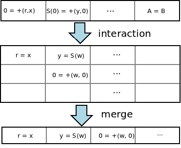
Figure 1: The interaction step

This approach is straightforward, but has performance drawbacks. The filter and merge operations on the result arrays are up to several hundred times slower than the actual parallel interaction step. This contributes to the current inefficiency of ingpu, which we shall discuss in detail in Section 4.

3.5 Parallel communication

After the interaction phase above has completed, we apply an algorithm corresponding to the communication rule to generate new active pairs. Recall the mechanics of $\;\stackrel{{\scriptstyle com}}{{\longrightarrow}}\;$: communication needs to find two equations $\{x=t,x=s\}$ where $x$ is a variable and $s,t$ are terms and merge them to a single equation $\{s=t\}$. Let us call two such equations sharing a variable communication-eligible. This is harder to parallelize than $\;\stackrel{{\scriptstyle int}}{{\longrightarrow}}\;$: we need to find eligible pairs of equations first before we reduce them. Unfortunately, this is where we run into a problem mentioned in Section 3.2: our net is only represented as an array of independent equations. There is no additional pointer structure between them to represent connections (cf. the Agent structure in Section 3.3). Therefore, we currently perform the following (inefficient) procedure to find communication-eligible pairs of equations: we sort all equations of the pattern $x=t$ by the id of the variable $x$. This places communication-eligible pairs of equations next to each other in the array (since the same variable occurs in them). We can now proceed to merge these pairs into single equations. We do this by using Thrust’s reduce_by_key(): this function essentially works like Haskell’s fold with an added predicate function. Only adjacent array elements that satisfy the predicate are folded. For example, consider a list of numbers $\{2,0,3,3,3,7,5,5\}$: calling reduce_by_key() on this list with addition as folding function and equality as predicate yields the result $\{2,0,9,7,10\}$.

Hence, we use having a common variable as reduce_by_key()’s predicate. This way, we merge communication-eligible pairs and leave all other equations untouched. The communication step can be summed up by the following pseudo-code:

⬇

let E be the array of all equations of shape x=t

sort E by the id of left part of each equation

reduce_by_key(E) with predicate p and reduce functor r

where

p (x,t) (y,s) = x==y

r (x,t) (y,s) = (s,t)

Thrust provides efficient implementations of parallel sorting algorithms, but sorting and reducing the equations still represents a major performance bottleneck for large inputs. We shall discuss this issue in detail in Section 4. For the remainder of this section, we shall show that our algorithm is correct.

3.6 Correctness of the algorithm

The communication algorithm seems fairly straightforward, but we have not discussed one important point: what if an equation consists of two variables, e.g. $x=t$ where $t$ is a variable? Which one is used for comparison in the sorting of the equations? Surprisingly, it does not matter for our algorithm. We shall now show that it is correct in the sense that any possible active pair that can be generated by $\;\stackrel{{\scriptstyle com}}{{\longrightarrow}}\;$in the lightweight calculus will also be generated by ingpu.

First however, we highlight that some active pairs cannot be generated by the communication algorithm described above. Consider a set of equations $\{A=x,x=y,y=B\}$. Clearly, both $x$ and $y$ can be resolved, yielding the active pair $A=B$. However, we need to perform two consecutive $\;\stackrel{{\scriptstyle com}}{{\longrightarrow}}\;$steps, first eliminating $x$ and then $y$ or the other way around. The communication algorithm above would only perform one of these communications, depending on whether $x$ or $y$ was used for sorting. The result would be $\{A=y,y=B\}$ (if x was reduced), which cannot be used in the interaction phase. A second pass of the communication algorithm would be necessary to yield the active equation $A=B$. The following pseudo-code of the evaluation function reflects this:

⬇

equation_list evaluate(equation_list L) {

transfer L to device (GPU) memory

do {

perform interaction as in Section 3.4

perform communication as in Section 3.5

}

while (at least one interaction or one communication

has occurred in the previous loop)

transfer L back to host (CPU) memory

return L

}

This way, if the communication algorithm does not yield any active pairs, it is performed again until it either generates new active pairs or no longer performs any $\;\stackrel{{\scriptstyle com}}{{\longrightarrow}}\;$steps. In the latter case, the program terminates. We can show that the algorithm is correct in the sense that it generates all possible active pairs and evaluates them.

Proposition 3.7 (Correctness of evaluate()).

Let $E$ be a set of equations such that there is an interaction rule for every active pair. Then, $R=$ evaluate($E$) contains no active pairs, and no further active pairs can be generated by applying $\;\stackrel{{\scriptstyle com}}{{\longrightarrow}}\;$in $R$.

Proof.

We show that for any set of equations that can potentially yield an active pair, evaluate() will generate this active pair. Such a set of equations has the general form $\{A=x_{1},\;x_{1}=x_{2},\;x_{2}=x_{3},\;\ldots,\;x_{i-1}=x_{i},\;x_{i}=B\}$. Applying the communication algorithm will result in at least one $\;\stackrel{{\scriptstyle com}}{{\longrightarrow}}\;$step, no matter which of the variables of each two-variable equation is used for sorting. Hence, the size of the set of equations decreases by at least 1 in each iteration of the loop in evaluate(). After at most $i$ loops, the communication algorithm will yield $\{A=B\}$, which can then be reduced in the subsequent interaction phase of evaluate(). ∎

Remark

Note that the algorithm may not be able to apply all $\;\stackrel{{\scriptstyle com}}{{\longrightarrow}}\;$steps to sets of equations that potentially do not yield an active pair. For example, $\{A=x_{1},\;x_{1}=x_{2},\;x_{2}=x_{3},\;\ldots,\;x_{i-1}=x_{i},\;x_{i}=y\}$ may not reduce to $\{A=y\}$ depending on the choice of comparison variables for sorting. However, these $\;\stackrel{{\scriptstyle com}}{{\longrightarrow}}\;$steps do not yield any active pairs and hence are of secondary importance, much like $\;\stackrel{{\scriptstyle col}}{{\longrightarrow}}\;$and $\;\stackrel{{\scriptstyle sub}}{{\longrightarrow}}\;$(cf. Theorem 1 in Section 2.2).

4 Benchmarks and future improvements

In this section, we present some benchmark results and discuss possible performance improvements. First, we compare ingpu to existing, sequential interaction nets evaluators. Second, we identify performance bottlenecks and discuss potential solutions.

4.1 Performance comparison

Our implementation is still considered experimental. Unfortunately, ingpu currently performs slower than the more mature sequential evaluators inets[9] and amineLight[6] in most cases. However, we can identify which parts of ingpu are slow and which ones are fast. Consider the benchmark comparison in Figure 2. We ran our tests on a machine with an Intel Core Duo 2.2Ghz CPU, 2GB of RAM and a Geforce GTX 460 graphics card.

time in seconds	amineLight	inets	ingpu
Ackermann(3,7)	0.4	0.59	30.4
Fibonacci(20)	0.03	0.043	10.5
L-System(27)	1.13	1.49	1.28

Figure 2: Benchmark results

On standard benchmark functions like Ackermann or Fibonacci, ingpu performs very poorly. The sequential implementations are much faster here. However, the result on the third benchmark L-System is much more competitive, at least outperforming inets. This set of rules computes the $n$th iteration of a basic L-System that models the growth of Algae [16], given by the following rewrite System:

$$A \rightarrow AB B \rightarrow A$$

So why is ingpu so much faster for the L-System ruleset? Two main reasons can be given, which at the same time highlight the most glaring performance problems:

Inefficient communication

Profiling shows that for Ackermann, almost all of the execution time of ingpu is spent in the communication phase and the merging part of the interaction phase. The actual interaction kernel (replacing equations) runs very fast, taking less than 0.1 percent of the total time.

Available parallelism

The term available parallelism was coined in [13], and refers to the number of expressions that can be evaluated in parallel at a given time during the execution of a program. In our case, this is simply the number of active pairs that exist at the same time at a certain iteration of ingpu’s main loop. A high number of active pairs fits the GPU programming model well, as GPUs are optimized to handle hundreds of thousands of data-parallel inputs. Conversely, a low amount of parallelism is not sufficient to leverage the full computing power of the GPU. Figure 3 shows the number of parallel interactions per loop for Ackermann and L-System. While Ackerman has less than 200 concurrent active pairs for the majority of its execution time, L-System performs several hundreds of thousands of parallel interactions towards the end of the computation. Moreover, L-System performs much fewer loop iterations overall (50 vs. 11000). This means that much less time is spent in the slow communication phase in proportion to the total number of interactions.

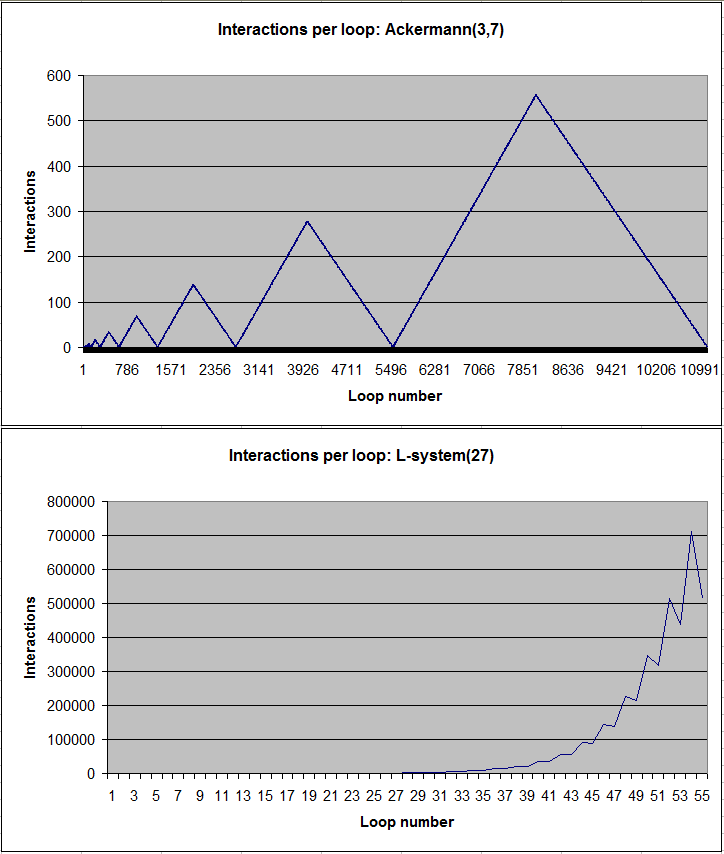
Figure 3: Available Parallelism of Ackermann and L-System: the $x$-axis shows the loop number, the $y$-axis the number of parallel interactions.

Figure 3 also gives some insight on the dynamics of available parallelism in our benchmarks. Interestingly, the number of concurrent active pairs for Ackermann repeatedly decreases and increases in a quasi oscillating fashion. This results in the rather low average number of active pairs per loop. In contrast, the available parallelism in the execution of L-System strongly increases, as is expected considering the exponential growth of the L-System. The slight drops in parallelism are the result of duplicating the parameter for the number of iterations in every loop.

4.2 Possible optimizations

Currently, ingpu is still in its experimental stages, and various small and big improvements can be made to increase its overall performance. In particular, we have identified a few optimizations that have the potential for a considerable performance increase. These are subject of current and future work.

Improved communication

As we discussed, our current communication algorithm is very slow. Due to the fact that an interaction net is represented as a list of independent equations, we have to sort the complete list repeatedly to find communication-eligible equations. However, it is possible to reduce this search space: only equations that are directly connected to a given active pair (i.e., its interface) are potentially communication-eligible. We gain a speedup by considering this subset of equations only. In order to efficiently determine the eligible equations, a pointer-based net representation in the GPU memory is needed (see the next paragraph).

A more efficient net representation

Both interaction and communication could benefit from a better net representation in the GPU memory. While the “array of equations” approach closely follows the theoretical definition of the interaction nets calculus, it is quite slow: the lack of a more sophisticated pointer structure makes a sorting pass in the communication phase necessary. We are currently implementing an approach where all agents and variables are stored in an array such that their unique id determines their array position. This way, we achieve constant-time access of agents and connections, making the sorting phase unnecessary.

Remove result array merging

The merging of the result vectors in the interaction phase (including dummy removal) could be improved by using CUDA’s atomic exchange operations: these functions allow individual kernel instances to read and write shared values. A shared pointer to the result vector could be provided to each thread. The threads could then add the dynamically-sized list of RHS equations to the result vector and update the pointer to the end of their output, removing the dummy removal pass.

A different approach to the problem of dynamic output size in GPU computations can be found in [11]: the authors propose a way to handle different output sizes without any communication between threads. The memory management in the output array is achieved by using parallel scan algorithms. We are currently adapting this approach to ingpu. Initial experiments show that this will indeed yield a considerable speedup.

5 Discussion

Related work

Evaluation of interaction nets can be considered an irregular algorithm, in the sense that it operates on a pointer structure (a graph) rather than a dense array. Bridging the conceptual gap between the irregular nature of interaction nets and the dense structure of typical GPU programs (e.g., dense matrix operations) is strongly related to the implementation challenges discussed in this paper. We have been inspired by the insights of parallelizing irregular algorithms in [13] when implementing ingpu. We also borrowed the term available parallelism from this work.

The efficient parallelization of general graph algorithms using GPUs has been the topic of several publications (for example, [8]). As part of future work, we plan to use these insights to achieve a better representation of interaction nets on the GPU.

Besides the previously mentioned inets and amineLight, several other interaction nets evaluators exist, for example [2, 12]. Another recent tool is PORGY [3], which can be used to analyse and evaluate interaction net systems with a focus on evaluation strategies. However, only few works (for example, [14]) on parallel evaluation of interaction nets exist. This is surprising, considering their potential for parallelism. To the best of our knowledge, there is no previous work on a GPU-based implementation.

With regard to functional programming in general, several systems based on GPUs have been developed. Two recent examples are Obsidian [15] and Accelerate [4], both being extensions of Haskell.

Conclusion

In this paper, we have presented ongoing work on ingpu, a GPU-based evaluator for interaction nets. This is a novel approach that heavily utilizes their potential for parallelism: all active pairs that are available at the same time are evaluated in parallel. Previous evaluators are sequential or only allow a fixed number of concurrent interactions (e.g., capped by the number of cores of the CPU). A GPU with hundreds of cores is better suited to perform a high number of small computations (i.e., reductions of active pairs). Still, the implementation poses a challenge due to the dynamic nature of interaction nets evaluation and the restrictions of the GPU computing model.

The work-in-progress status of ingpu is clearly visible in the benchmark results of Section 4. While parallel evaluation is generally expected to be faster than a sequential one, our current implementation mostly performs weaker than existing evaluators. However, we argue that the potential of ingpu can be seen in the difference between the individual results. In our L-System test, ingpu performs more than 50 times faster than for Ackermann, in terms of interactions per second. The major part of the slowdown is caused by the communication phase, which should be seen as an intermediate solution. In contrast to this, the interaction phase (parallel reduction of the active pairs) is very fast and shows that interaction nets and GPU are a promising match.

For current and future work, we plan to optimize the system to improve the obvious performance bottlenecks. Initial tests show that with a more efficient net representation in GPU memory and the removal of result array merging (see Section 4.2), ingpu strongly outperforms CPU-based systems at least for highly parallel benchmarks.

References

- [1]
- [2] Jose Bacelar Almeida, Jorge Sousa Pinto & Miguel Vilaca (2008): A tool for programming with interaction nets. Electronic Notes in Theoretical Computer Science 219, pp. 83–96, 10.1016/j.entcs.2008.10.036.
- [3] Oana Andrei, Maribel Fernández, Hélène Kirchner, Guy Melançon, Olivier Namet & Bruno Pinaud (2011): PORGY: Strategy-Driven Interactive Transformation of Graphs. In Rachid Echahed, editor: Proceedings 6th International Workshop on Computing with Terms and Graphs, Saarbrücken, Germany, 2nd April 2011, Electronic Proceedings in Theoretical Computer Science 48, pp. 54–68, 10.4204/EPTCS.48.7.
- [4] Manuel M. T. Chakravarty, Gabriele Keller, Sean Lee, Trevor L. McDonell & Vinod Grover (2011): Accelerating Haskell array codes with multicore GPUs. In Manuel Carro & John H. Reppy, editors: Proceedings of the POPL 2011 Workshop on Declarative Aspects of Multicore Programming, DAMP 2011, Austin, TX, USA, January 23, 2011, pp. 3–14, 10.1145/1926354.1926358.
- [5] Maribel Fernández & Ian Mackie (1999): A Calculus for Interaction Nets. In Gopalan Nadathur, editor: Principles and Practice of Declarative Programming, International Conference PPDP’99, Paris, France, September 29–October 1, 1999, Proceedings, Lecture Notes in Computer Science 1702, Springer, pp. 170–187, 10.1007/10704567_10.
- [6] Abubakar Hassan, Ian Mackie & Shinya Sato (2010): A lightweight abstract machine for interaction nets. Electronic Communication of the European Association of Software Science and Technology 29.
- [7] Jared Hoberock & Nathan Bell (2010): Thrust: A Parallel Template Library. Available at http://www.meganewtons.com/. Version 1.3.0.
- [8] Sungpack Hong, Sang Kyun Kim, Tayo Oguntebi & Kunle Olukotun (2011): Accelerating CUDA graph algorithms at maximum warp. In Calin Cascaval & Pen-Chung Yew, editors: Proceedings of the 16th ACM SIGPLAN Symposium on Principles and Practice of Parallel Programming, PPOPP 2011, San Antonio, TX, USA, February 12-16, 2011, pp. 267–276, 10.1145/1941553.1941590.
- [9] The Inets Project site [Online, accessed 13-April-2012]. http://gna.org/projects/inets.
- [10] Yves Lafont (1990): Interaction Nets. In Frances E. Allen, editor: Conference Record of the Seventeenth Annual ACM Symposium on Principles of Programming Languages, San Francisco, California, USA, January 1990, ACM, pp. 95–108, 10.1145/96709.96718.
- [11] Markus Lipp, Peter Wonka & Michael Wimmer (2010): Parallel generation of multiple L-systems. Computers & Graphics 34(5), pp. 585–593, 10.1016/j.cag.2010.05.014.
- [12] Sylvain Lippi (2002): in : A Graphical Interpreter for Interaction Nets. In Sophie Tison, editor: Rewriting Techniques and Applications, 13th International Conference, RTA 2002, Copenhagen, Denmark, July 22-24, 2002, Proceedings, Lecture Notes in Computer Science 2378, pp. 380–386, 10.1007/3-540-45610-4_29.
- [13] Mario Méndez-Lojo, Donald Nguyen, Dimitrios Prountzos, Xin Sui, Muhammad Amber Hassaan, Milind Kulkarni, Martin Burtscher & Keshav Pingali (2010): Structure-driven optimizations for amorphous data-parallel programs. In R. Govindarajan, David A. Padua & Mary W. Hall, editors: Proceedings of the 15th ACM SIGPLAN Symposium on Principles and Practice of Parallel Programming, PPOPP 2010, Bangalore, India, January 9-14, 2010, pp. 3–14, 10.1145/1693453.1693457.
- [14] Jorge Sousa Pinto (2001): Parallel Evaluation of Interaction Nets with MPINE. In Aart Middeldorp, editor: Rewriting Techniques and Applications, 12th International Conference, RTA 2001, Utrecht, The Netherlands, May 22-24, 2001, Proceedings, Lecture Notes in Computer Science 2051, pp. 353–356, 10.1007/3-540-45127-7_26.
- [15] Joel Svensson, Koen Claessen & Mary Sheeran (2010): GPGPU kernel implementation and refinement using Obsidian. Procedia Computer Science 1(1), pp. 2065–2074, 10.1016/j.procs.2010.04.231.
- [16] Wikipedia (2011): L-system — Wikipedia, The Free Encyclopedia [Online, accessed 23-November-2011]. http://en.wikipedia.org/wiki/L-system.