Quantum Turing automata

Abstract

A denotational semantics of quantum Turing machines having a quantum control is defined in the dagger compact closed category of finite dimensional Hilbert spaces. Using the Moore-Penrose generalized inverse, a new additive trace is introduced on the restriction of this category to isometries, which trace is carried over to directed quantum Turing machines as monoidal automata. The Joyal-Street-Verity $Int$ construction is then used to extend this structure to a reversible bidirectional one.

1 Introduction

In recent years, following the endeavors of Abramsky and Coecke to express some of the basic quantum-mechanical concepts in an abstract axiomatic category theory setting, several models have been worked out to capture the semantics of quantum information protocols [2] and programming languages [13, 17, 25]. Concerning quantum hardware, an algebra of automata which include both classical and quantum entities has been studied in [14]. In all of these works, while the model could manipulate quantum data structures, the actual control flow of the data was assumed to be necessarily classical.

The objective of the present paper is to show that the idea of a quantum control is logically sound and feasible, and to provide a denotational style semantics for quantum Turing machines having such a control. At the same time, the rigid topological layout of Turing machines as a linear array of tape cells is replaced by a flexible graph structure, giving rise to the concept of Turing automata and graph machines as introduced in [7]. By denotational semantics we mean that the changing of the tape contents caused by the entire computation process is specified directly as a linear operator, rather than just one step of this process.

Our presentation will use the language of [2, 18, 24], but it will be specific to the concrete dagger compact closed category $(\mbox{\bf FdHilb},\otimes)$ of finite dimensional Hilbert spaces at this time. One can actually read Section 4 separately as an interesting study in linear algebra, introducing a novel application of the Moore-Penrose generalized inverse of range-Hermitian operators by taking their Schur complement in certain block matrix operators. This is the main technical contribution of the paper. We believe, however, that the category theory contributions are far more interesting and relevant. All of these results are around the well-known Geometry of Interaction (GoI) concept introduced originally by Girard [15] in the late 1980’s as an interpretation of linear logic. The ideas, however, originate from and are directly related to a yet earlier work [3] by the author on the axiomatization of flowchart schemes, where the traced monoidal category axioms first appeared in an algebraic context. Our category theory contributions are as follows:

1. We introduce a total trace on the monoidal subcategory of $(\mbox{\bf FdHilb},\oplus)$ defined by isometries, which has previously been sought by others [16, 22].

2. We explain the role of the $Int$ construction for traced monoidal categories [18] in turning a computation process bidirectional or reversible.

3. We capture the phenomenon in (ii) above by our own concept “indexed monoidal algebra” [8], which is an equivalent formalism for certain regular self-dual compact closed categories.

Due to space limitations we have to assume familiarity with some advanced concepts in category theory, namely traced monoidal categories [18], compact closed categories [20], and the $Int$ construction that links these two types of symmetric monoidal categories [21] to each other. For brevity, by a monoidal category we shall mean a symmetric monoidal one throughout the paper.

2 Traced and compact closed monoidal categories

The following definition of (strict) traced monoidal categories uses the terminology of [18]. Trace (called feedback in [3]) in a monoidal category $\mathcal{C}$ with unit object $I$, tensor $\otimes$, and symmetries $c_{A,B}:A\otimes B\rightarrow B\otimes A$ is introduced as a left trace, i.e., an operation $\mathcal{C}(U\otimes A,U\otimes B)\rightarrow\mathcal{C}(A,B)$.

Definition 1.

A trace for a monoidal category $\mathcal{C}$ is a family of functions

$$\mathrm{Tr}_{A,B}^{U}:\mathcal{C}(U\otimes A,U\otimes B)\rightarrow\mathcal{C}(A,B)$$

natural in $A$ and $B$, dinatural in $U$, and satisfying the following three axioms:

vanishing:

$$\mathrm{Tr}_{A,B}^{I}(f)=f\;,\;\;\;\mathrm{Tr}_{A,B}^{U\otimes V}(g)=\mathrm{Tr}_{A,B}^{V}(\mathrm{Tr}_{V\otimes A,V\otimes B}^{U}(g));$$

superposing:

$$\mathrm{Tr}_{A,B}^{U}(f)\otimes g=\mathrm{Tr}_{A\otimes C,B\otimes D}^{U}(f\otimes g),\mbox{\ where\ }g:C\rightarrow D;$$

yanking:

$$\mathrm{Tr}_{U,U}^{U}(c_{U,U})=1_{U}.$$

We use the word sliding as a synonym for dinaturality in $U$. When using the term feedback for trace, the notation $\mathrm{Tr}$ changes to $\uparrow$ or ${\Uparrow}$, and we simply write $\mathrm{Tr}^{U}$ ($\uparrow^{U}$, ${\Uparrow}^{U}$) for $\mathrm{Tr}_{A,B}^{U}$ whenever $A$ and $B$ are understood from the context. The reason for using three different symbols for trace is the different nature of semantics associated with these symbols.

As it is customary in linear algebra, we shall use the symbols $I$ and $0$ as “generic” identity (respectively, zero) operators, provided that the underlying Hilbert space is understood from the context. As a further technical simplification we shall be working with the strict monoidal formalism, even though the monoidal category of Hilbert spaces with the usual tensor product is not strict. It is known, cf. [21], that every monoidal category is equivalent to a strict one.

Definition 2.

A monoidal category $\mathcal{C}$ is compact closed (CC, for short) if every object $A$ has a left adjoint $A^{*}$ in the sense that there exist morphisms $d_{A}:I\rightarrow A^{*}\otimes A$ (the unit map) and $e_{A}:A\otimes A^{*}\rightarrow I$ (the counit map) for which the two composites below result in the identity morphisms $1_{A}$ and $1_{A^{*}}$, respectively.

$$A \!\!\!\!= \!\!\!\!A\otimes I\rightarrow_{1_{A}\otimes d_{A}}A\otimes(A^{*}\otimes A)=(A\otimes A^{*})\otimes A\rightarrow_{e_{A}\otimes 1_{A}}I\otimes A=A,$$

$$A^{*} \!\!\!\!= \!\!\!\!I\otimes A^{*}\rightarrow_{d_{A}\otimes 1_{A^{*}}}(A^{*}\otimes A)\otimes A^{*}=A^{*}\otimes(A\otimes A^{*})\rightarrow_{1_{A^{*}}\otimes e_{A}}A^{*}\otimes I=A^{*}.$$

As it is well-known, every CC category admits a so called canonical trace [18] defined by the formula

$$\mathrm{Tr}_{A,B}^{U}f=(d_{U}\otimes 1_{A})\circ(1_{U^{*}}\otimes f)\circ(e_{U^{*}}\otimes 1_{B}).$$

Notice that we write composition of morphisms ($\circ$) in a left-to-right order, avoiding the use of “;”, which some may find more appropriate. We do so in order to facilitate a smooth transition from composition to matrix product in Section 4. In the formula of canonical trace above we have made the additional silent assumption that the involution $()^{*}$ is strict, so that $U^{**}=U$ holds for each object $U$. As it is known from [12], this assumption can also be made without loss of generality.

Recall from [24] that a dagger monoidal category is a monoidal category $\mathcal{C}$ equipped with an involutive, identity-on-objects contravariant functor ${}^{\dagger}:\mathcal{C}^{op}\rightarrow\mathcal{C}$ coherently preserving the symmetric monoidal structure as specified in [24]. A dagger compact closed category is a dagger monoidal category that is also compact closed, and such that the diagram in Figure 1 commutes for all objects $A$.

Figure 1: Diagram for dagger compact closed categories

3 Monoidal vs. Turing automata

Circuits and automata over an arbitrary monoidal category $M$ have been studied in [4, 5, 6, 19]. It was shown that the collection of such machines has the structure of a monoidal category equipped with a natural feedback operation, which satisfies the traced monoidal axioms, except for yanking. Moreover, sliding holds in a weak sense, for isomorphisms only.

Let $A$ and $B$ be objects in $M$. An $M$-automaton (circuit) $A\rightarrow B$ is a pair $(U,\alpha)$, where $U$ is a further object and $\alpha:U\otimes A\rightarrow U\otimes B$ is a morphism in $M$. If, for example, $M=(\mbox{\bf Set},\times)$, then the pair $(U,\alpha)$ represents a deterministic Mealy automaton with states $U$, input $A$, and output $B$. The structure of $M$-automata/circuits has been described as a monoidal category $\mathrm{Circ}(M)$ with feedback in [19]. This category was also shown to be freely generated by $M$.

In this paper we take a different approach to the study of monoidal automata. We follow the method of [7] with the aim of constructing a traced monoidal category as an adequate semantical structure for these automata. One must not confuse this type of semantics with the meaning normally associated with the category $\mathrm{Circ}(M)$ above, as they have seemingly very little in common. A traced monoidal category indicates a delay-free semantics, as opposed to the step-by-step delayed semantics suggested by $\mathrm{Circ}(M)$. Moreover, the category that we are going to construct is not meant to be the quotient of $\mathrm{Circ}(M)$ by the yanking identity, so as to turn it into a traced monoidal category in the straightforward manner. Rather, we define a brand new tensor and feedback (trace) on our $M$-automata, which are analogous to the basic operations in iteration theories [11]. Regarding the base category $M$, we shall assume an additional, so called additive tensor $\oplus$, so that $\otimes$ distributes over $\oplus$. These two tensors will then be “mixed and matched” in the definition of tensor for $M$-automata, providing them with an intrinsic Turing machine behavior.

The “prototype” of this construction, resulting in the CC category of conventional Turing automata, has been elaborated in [8] using $M=(\mbox{\bf Rel},\times,+)$ as the base category. This category was ideal as a template for the kind of construction we have in mind, since it has a biproduct $+$ as the additive tensor and is self-dual compact closed according to the multiplicative tensor $\times$. Below we present the quantum counterpart of this construction, working in the dagger compact closed category of finite dimensional Hilbert spaces $(\mbox{\bf FdHilb},\otimes,\oplus)$. More precisely, the category $M$ above will be the restriction of FdHilb to isometries as morphisms, which subcategory is no longer compact closed and does not have a biproduct.

4 Directed quantum Turing automata

In this section we present the construction outlined above, to obtain a strange asymmetric model which does not yet qualify as a recognizable quantum computing device in its own right. The model represents a Turing machine in which cells are interconnected in a directed way, so that the control (tape head) always moves along interconnections in the given fixed direction, should it be left or right. In other words, direction is incorporated in the scheme-like graphical syntax, rather than the semantics. We use this model only as a stepping stone towards our real objective, the (undirected) quantum Turing automaton described in Section 5.

Definition 3.

A directed quantum Turing automaton is a quadruple

$$T=(\mathcal{H},\mathcal{K},\mathcal{L},\tau),$$

where $\mathcal{H}$, $\mathcal{K}$, and $\mathcal{L}$ are finite dimensional Hilbert spaces over the complex field $\mathbb{C}$, and $\tau:\mathcal{H}\otimes\mathcal{K}\rightarrow\mathcal{H}\otimes\mathcal{L}$ is an isometry in FdHilb.

Recall that an isometry between Hilbert spaces $\mathcal{H}_{1}$ and $\mathcal{H}_{2}$ is a linear map $\sigma:\mathcal{H}_{1}\rightarrow\mathcal{H}_{2}$ such that $\sigma\circ\sigma^{\dagger}=I$, where $\sigma^{\dagger}$ is the (Hilbert space) adjoint of $\sigma$. Following the notation of general monoidal automata we write $T:\mathcal{K}\rightarrow\mathcal{L}$, and call the isometry $\tau$ the transition operator of $T$. Thus, $T$ is the monoidal automaton $(\mathcal{H},\tau):\mathcal{K}\rightarrow\mathcal{L}$. Sometimes we simply identify $T$ with $\tau$, provided that the other parameters of $T$ are understood from the context.

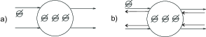
Figure 2: Two simple DQTA

The reader can obtain an intuitive understanding of the automaton $T$ from Figure 2a. The state space $\mathcal{H}$ is represented by a finite number of qubits (in our example 3), while the control is a moving particle that moves from one of the input interfaces (space $\mathcal{K}$) to one of the output ones (space $\mathcal{L}$). It can only move in the input $\rightarrow$ output direction, as specified by the operator $\tau$. The number of input and output interfaces is finite. The control itself does not carry any information, it is just moving around and changes the state of $T$. In comparison with conventional Turing machines, the state of $T$ is the tape contents of the corresponding Turing machine, and the current state of the Turing machine is just an interface identifier for $T$. For example, one can consider the DQTA in Figure 2b as one tape cell of a Turing machine $TM$ having $2^{3}$ symbols in its tape alphabet and only 2 states (2 left-moving and 2 right-moving interfaces, both input and output). Correspondingly, $\mathcal{H}$ is $8$-dimensional, while the dimension of both $\mathcal{K}$ and $\mathcal{L}$ is $4$. In motion, if the control particle of $T$ resides on the input interface labeled $(L,i)$ ($(R,i)$), then $TM$ is in state $i$ moving to the left (respectively, right). The point is, however, that the automaton $T$ need not represent just one cell, it could stand for any finite segment of a Turing machine, in fact a Turing graph machine in the sense of [7]. In our concrete example, a segment of $TM$ with $n$ tape cells would have $3n$ qubits inside the circle of Figure 2b, but still the same $4+4$ interfaces.

An isometric isomorphism $\sigma:\mathcal{H}_{1}\rightarrow\mathcal{H}_{2}$ (unitary map, if $\mathcal{H}_{1}=\mathcal{H}_{2}$) is a linear operator such that both $\sigma$ and $\sigma^{\dagger}$ are isometries. Two automata $T_{i}:(\mathcal{H}_{i},\tau_{i}):\mathcal{K}\rightarrow\mathcal{L}$, $i=1,2$, are isomorphic, notation $T_{1}\cong T_{2}$, if there exists an isometric isomorphism $\sigma:\mathcal{H}_{1}\rightarrow\mathcal{H}_{2}$ for which

$$\tau_{2}=(\sigma^{\dagger}\otimes I_{\mathcal{K}})\circ\tau_{1}\circ(\sigma\otimes I_{\mathcal{L}}).$$

For simplicity, though, we shall work with representatives, rather than equivalence classes of automata.

Turing automata can be composed by the standard cascade product of monoidal automata, cf. [5, 6, 19]. If $T_{1}=(\mathcal{H}_{1},\tau_{1}):\mathcal{L}\rightarrow\mathcal{M}$ and $T_{2}=(\mathcal{H}_{2},\tau_{2}):\mathcal{M}\rightarrow\mathcal{N}$ are directed quantum Turing automata (DQTA, for short), then

$$T_{1}\circ T_{2}=(\mathcal{H}_{1}\otimes\mathcal{H}_{2},\mathcal{L},\mathcal{N},\tau)$$

is the automaton whose transition operator $\tau$ is

$$(\pi_{\mathcal{H}_{1},\mathcal{H}_{2}}\otimes I_{\mathcal{L}})\circ(I_{\mathcal{H}_{2}}\otimes\tau_{1})\circ(\pi_{\mathcal{H}_{2},\mathcal{H}_{1}}\otimes I_{\mathcal{M}})\circ(I_{\mathcal{H}_{1}}\otimes\tau_{2}),$$

where $\pi_{\mathcal{H},\mathcal{K}}$ is the symmetry $\mathcal{H}\otimes\mathcal{K}\rightarrow\mathcal{K}\otimes\mathcal{H}$ in $(\mbox{\bf FdHilb},\otimes)$. As known from [19], the cascade product of automata is compatible with isomorphism, so that it is well-defined on isomorphism classes of DQTA. The identity Turing automaton $1_{\mathcal{K}}:\mathcal{K}\rightarrow\mathcal{K}$ has the unit space $\mathbb{C}$ as its state space, and its transition operator is simply $I_{\mathcal{K}}$. The results in [19] imply that these data define a category DQT over finite dimensional Hilbert spaces as objects, in which the morphisms are isomorphism classes of DQTA.

Now let

$$T_{1}=(\mathcal{H}_{1},\tau_{1}):\mathcal{K}_{1}\rightarrow\mathcal{L}_{1}\mbox{\ and\ }T_{2}=(\mathcal{H}_{2},\tau_{2}):\mathcal{K}_{2}\rightarrow\mathcal{L}_{2}$$

be DQTA, and define $T_{1}\boxplus T_{2}$ to be the automaton over the state space $\mathcal{H}_{1}\otimes\mathcal{H}_{2}$ whose transition operator

$$\tau=\tau_{1}\boxplus\tau_{2}:(\mathcal{H}_{1}\otimes\mathcal{H}_{2})\otimes(\mathcal{K}_{1}\oplus\mathcal{K}_{2})\rightarrow(\mathcal{H}_{1}\otimes\mathcal{H}_{2})\otimes(\mathcal{L}_{1}\oplus\mathcal{L}_{2})$$

acts as follows: $\tau\simeq\sigma_{1}\oplus\sigma_{2}$, where the morphisms

$$\sigma_{i}:(\mathcal{H}_{1}\otimes\mathcal{H}_{2})\otimes\mathcal{K}_{i}\rightarrow(\mathcal{H}_{1}\otimes\mathcal{H}_{2})\otimes\mathcal{L}_{i},\,\,\,\,i=1,2\mbox{\ are:}$$

$$\sigma_{1}=(\pi_{\mathcal{H}_{1},\mathcal{H}_{2}}\otimes I_{\mathcal{K}_{1}})\circ(I_{\mathcal{H}_{2}}\otimes\tau_{1})\circ(\pi_{\mathcal{H}_{2},\mathcal{H}_{1}}\otimes I_{\mathcal{L}_{1}}),\mbox{\ \ and\ \ }\sigma_{2}=I_{\mathcal{H}_{1}}\otimes\tau_{2}.$$

In the above equations, $\oplus$ denotes the orthogonal sum of Hilbert spaces. Intuitively, $\tau$ is the selective performance of either $\tau_{1}$ or $\tau_{2}$ on the tensor space $\mathcal{H}_{1}\otimes\mathcal{H}_{2}$. We say “either or”, because the interfaces of $T_{1}$ and $T_{2}$ are separated by $\oplus$, rather than $\otimes$. The natural isomorphism $\simeq$ is distributivity in the sense of [2, Proposition 5.3]. It is clear that the operator $\tau_{1}\boxplus\tau_{2}$ is an isometry, so that the operation $\boxplus$ is well-defined. We call this operation the Turing tensor. The Turing tensor is also associative, up to natural isomorphism, of course.

The symmetries $\mathcal{K}\oplus\mathcal{L}\rightarrow\mathcal{L}\oplus\mathcal{K}$ associated with $\boxplus$ are the “single-state” Turing automata whose transition operator is the permutation

$$\kappa_{\mathcal{K},\mathcal{L}}=\!\!\!\begin{array}[]{cc}&\begin{array}[]{cc}\mathcal{L}&\mathcal{K}\end{array}\\ \begin{array}[]{c}\mathcal{K}\\ \mathcal{L}\end{array}&\!\!\!\!\!\left(\begin{array}[]{cc}0&I\\ I&0\end{array}\right)\end{array}\!\!:(\mathbb{C}\otimes)(\mathcal{K}\oplus\mathcal{L})\rightarrow(\mathbb{C}\otimes)(\mathcal{L}\oplus\mathcal{K}).$$

Along the lines of [19] it is routine to check that $\boxplus$ is also compatible with isomorphism of automata, and $(\mbox{\bf DQT},\boxplus)$ becomes a monoidal category in this way.

Our third basic operation on DQTA is feedback. Feedback follows the scheme of iteration in Conway matrix theories [11], using an appropriate star operation. Let $T:\mathcal{U}\oplus\mathcal{K}\rightarrow\mathcal{U}\oplus\mathcal{L}$ be a DQTA having

$$\tau:\mathcal{H}\otimes(\mathcal{U}\oplus\mathcal{K})\rightarrow\mathcal{H}\otimes(\mathcal{U}\oplus\mathcal{L})$$

as its transition operator. Then $\uparrow^{\mathcal{U}}T:\mathcal{K}\rightarrow\mathcal{L}$ is the automaton over (the same space) $\mathcal{H}$ specified as follows. Consider the matrix of $\tau$:

$$\begin{array}[]{cc}&\begin{array}[]{cc}\mathcal{H}\otimes\mathcal{U}&\mathcal{H}\otimes\mathcal{L}\end{array}\\ \begin{array}[]{c}\mathcal{H}\otimes\mathcal{U}\\ \mathcal{H}\otimes\mathcal{K}\end{array}&\!\!\!\!\left(\begin{array}[]{cccccc}&\tau_{A}&&&\tau_{B}&\\ &\tau_{C}&&&\tau_{D}&\end{array}\right)\end{array}$$

according to the biproduct decomposition

$$\tau=\langle[\tau_{A},\tau_{C}],[\tau_{B},\tau_{D}]\rangle,$$

where $[\_\,,\_\,]$ stands for coproduct and $\langle\_\,,\_\,\rangle$ for product. The transition operator of $\uparrow^{\mathcal{U}}T$ is defined by the Kleene formula:

$$\uparrow^{\mathcal{U}}\tau=\lim_{n\rightarrow\infty}(\tau_{D}+\tau_{C}\circ\tau_{A}^{*n}\circ\tau_{B}).$$ (1)

In the Kleene formula, $\tau_{A}^{*n}=\sum_{i=0}^{n}\tau_{A}^{i}$, where $\tau_{A}^{0}=I$ and $\tau_{A}^{i+1}=\tau_{A}^{i}\circ\tau_{A}$. In other words, $\tau_{A}^{*n}$ is the $n$-th approximation of $\tau_{A}$’s Neumann series well-known in operator theory. The correctness of the above definition is contingent upon the existence of the limit and also on the resulting operator being an isometry. For these two conditions we need to make a short digression, which will also clarify the linear algebraic background.

Let Iso denote the subcategory of FdHilb having only isometries as its morphisms. Notice that $(\mbox{\bf{Iso}},\otimes)$ is no longer compact closed, even though the multiplicative tensor $\otimes$ is still intact in it. (The duals are gone.) This tensor, however, does not concern us at the moment. Consider $\oplus$ as an additive tensor in Iso:

$$\tau_{1}\oplus\tau_{2}=\langle[\tau_{1},0],[0,\tau_{2}]\rangle\mbox{\ \ for all isometries $\tau_{i}:\mathcal{H}_{i}\rightarrow\mathcal{K}_{i}$, $i=1,2$.}$$

Clearly, $\tau_{1}\oplus\tau_{2}$ is an isometry. The new additive unit (zero) object is the zero space $\mathcal{Z}$. With the additive symmetries $\kappa_{\mathcal{H},\mathcal{K}}:\mathcal{H}\oplus\mathcal{K}\rightarrow\mathcal{K}\oplus\mathcal{H}$, $(\mbox{\bf{Iso}},\oplus)$ again qualifies as a monoidal category. The biproduct property of $\oplus$ is lost, however. Nevertheless, one may attempt to define a trace operation $\uparrow^{\mathcal{U}}\tau$ in Iso by the Kleene formula (1), where $\tau:\mathcal{U}\oplus\mathcal{K}\rightarrow\mathcal{U}\oplus\mathcal{L}$. (Cut $\mathcal{H}\otimes$ in the matrix of $\tau$.)

Since the Kleene formula does not appear to be manageable, we first redefine $\uparrow^{\mathcal{U}}\tau$ and prove the equivalence of the two definitions later. Let

$${\Uparrow}^{\mathcal{U}}\tau=\tau_{D}+\tau_{C}\circ(I-\tau_{A})^{+}\circ\tau_{B},$$ (2)

where $(\,)^{+}$ denotes the Moore-Penrose generalized inverse of linear operators. Recall, e.g., from [9] that the Moore-Penrose inverse (MP inverse, for short) of an arbitrary operator $\sigma:\mathcal{H}\rightarrow\mathcal{K}$ is the unique operator $\sigma^{+}:\mathcal{K}\rightarrow\mathcal{H}$ satisfying the following two conditions:

1. $\sigma\circ\sigma^{+}\circ\sigma=\sigma$, and $\sigma^{+}\circ\sigma\circ\sigma^{+}=\sigma^{+}$;

2. $\sigma\circ\sigma^{+}$ and $\sigma^{+}\circ\sigma$ are Hermitian.

The connection between formulas (1) and (2) is the following. If the Neumann series $\tau_{A}^{*}$ converges, then $(I-\tau_{A})$ is invertible and

$$\tau_{A}^{*}=(I-\tau_{A})^{-1}=(I-\tau_{A})^{+}.$$

We know that $\|\tau_{A}\|\leq 1$, where $\|\,\|$ denotes the operator norm. ($\tau$ is an isometry.) Therefore the Kleene formula needs an explanation only if $\|\tau_{A}\|=1$. In that case, even if $(I-\tau_{A})$ is invertible, $\tau_{A}^{*}$ may not converge.

Just as the Kleene formula in computer science, the expression on the right-hand side of equation (2) is well-known and frequently used in linear algebra. For a block matrix

$$M=\left(\begin{array}[]{cc}A&B\\ C&D\end{array}\right),$$

where $A$ is square, the matrix $D-CA^{+}B$ is called the Schur complement of $A$ on $M$, denoted $A/M$. Cf., e.g., [9]. Observe that, under the assumption $\mathcal{K}=\mathcal{L}$,

$${\Uparrow}^{\mathcal{U}}\tau=I-(I-\tau_{A})/(I-\tau).$$

For this reason we call ${\Uparrow}^{\mathcal{U}}\tau$ the Schur I-complement of $\tau_{A}$ on $\tau$, and write ${\Uparrow}^{\mathcal{U}}\tau=\tau_{A}\backslash\tau$.

Theorem 4.

The operator $\tau_{A}\backslash\tau$ is an isometry.

Proof. Isolate the kernel $\mathcal{N}$ of $(I-\tau_{A})$, and let $\mathcal{U}_{0}$ be the orthogonal complement [23] of $\mathcal{N}$ on $\mathcal{U}$. The matrix of $(I-\tau_{A})$ in this breakdown is

$$I-\tau_{A}=\!\!\begin{array}[]{cc}&\begin{array}[]{ccc}\mathcal{N}&&\mathcal{U}_{0}\end{array}\\ \begin{array}[]{c}\mathcal{N}\\ \mathcal{U}_{0}\end{array}&\left(\begin{array}[]{cc}0&0\\ -\tau_{A}^{\mathcal{N}}&I-\tau_{A}^{0}\end{array}\right)\end{array}.$$ (3)

Put this matrix (rather, $I-(I-\tau_{A})$) in the top left corner of $\tau$:

$$\begin{array}[]{cc}&\begin{array}[]{ccccc}\mathcal{N}&&\mathcal{U}_{0}&&\mathcal{L}\end{array}\vspace*{1ex}\\ \begin{array}[]{c}\mathcal{N}\vspace*{1ex}\\ \mathcal{U}_{0}\vspace*{1ex}\\ \mathcal{K}\end{array}&\left(\begin{array}[]{ccccc}I&&0&&\tau_{B}^{\mathcal{N}}\vspace*{1ex}\\ \tau_{A}^{\mathcal{N}}&&\tau_{A}^{0}&&\tau_{B}^{0}\vspace*{1ex}\\ \tau_{C}^{\mathcal{N}}&&\tau_{C}^{0}&&\tau_{D}\end{array}\right)\end{array}.$$

Since $\tau$ is an isometry (regardless of its concrete orthogonal representation as a matrix operator), all entries in the above block matrix with superscript $\mathcal{N}$ must be $0$. Consequently, $(I-\tau_{A}^{0})$ is invertible and $\tau_{A}\backslash\tau=\tau_{A}^{0}\backslash\tau_{0}$, where $\tau_{0}:\mathcal{U}_{0}\oplus\mathcal{K}\rightarrow\mathcal{U}_{0}\oplus\mathcal{L}$ is the restriction of $\tau$ to the bottom right $2\times 2$ corner. Indeed,

$$\left(\begin{array}[]{ccc}0&&0\\ 0&&I-\tau_{A}^{0}\end{array}\right)^{+}=\left(\begin{array}[]{ccc}0&&0\\ 0&&(I-\tau_{A}^{0})^{-1}\end{array}\right),$$

so that

$$\tau_{C}\circ(I-\tau_{A})^{+}\circ\tau_{B}=\tau_{C}^{0}\circ(I-\tau_{A}^{0})^{-1}\circ\tau_{B}^{0}.$$

It turns out from the above discussion that $(I-\tau_{A})$ is group invertible and range-Hermitian, cf. [9, 10]. Therefore the MP inverse of $(I-\tau_{A})$ coincides with its Drazin inverse, which is the group generalized inverse of this operator. Cf. again [9, 10]. It follows that we can assume, without loss of generality, that $(I-\tau_{A})$ is invertible. Note that (3) is only a unitary similarity, therefore the sliding axiom is needed to make this argument correct. Cf. Theorem 7 below. For better readability, replace the symbols $\tau_{A}$, $\tau_{B}$, $\tau_{C}$, and $\tau_{D}$ by $A$, $B$, $C$, and $D$, respectively. Furthermore, ignore the composition symbol $\circ$ as if we were dealing with ordinary matrix product. Then we have:

$$\left(\begin{array}[]{cc}A&B\\ C&D\end{array}\right)\left(\begin{array}[]{cc}A^{\dagger}&C^{\dagger}\\ B^{\dagger}&D^{\dagger}\end{array}\right)=\left(\begin{array}[]{cc}I&0\\ 0&I\end{array}\right).$$

The following four matrix equations are derived:

$$AA^{\dagger}+BB^{\dagger} = I,$$ (4)

$$AC^{\dagger}+BD^{\dagger} = 0,$$ (5)

$$CA^{\dagger}+DB^{\dagger} = 0,$$ (6)

$$CC^{\dagger}+DD^{\dagger} = I.$$ (7)

We need to show that

$$(D+C(I-A)^{-1}B)(D^{\dagger}+B^{\dagger}(I-A^{\dagger})^{-1}C^{\dagger})=I.$$

The product on the left-hand side yields:

$$DD^{\dagger}+DB^{\dagger}(I-A^{\dagger})^{-1}C^{\dagger}+C(I-A)^{-1}BD^{\dagger}+C(I-A)^{-1}BB^{\dagger}(I-A^{\dagger})^{-1}C^{\dagger}.$$

By (5) and (6) this is equal to:

$$DD^{\dagger}-CA^{\dagger}(I-A^{\dagger})^{-1}C^{\dagger}-C(I-A)^{-1}AC^{\dagger}+C(I-A)^{-1}BB^{\dagger}(I-A^{\dagger})^{-1}C^{\dagger},$$

which is further equal to $DD^{\dagger}+CQC^{\dagger}$, where

$$Q\!=\!(I-A)^{-1}BB^{\dagger}(I-A^{\dagger})^{-1}\!-A^{\dagger}(I-A^{\dagger})^{-1}\!-(I-A)^{-1}A.$$

According to (7) it is sufficient to prove that $Q=I$. A couple of equivalent transformations follow. Multiply both sides of $Q=I$ by $(I-A)$ from the left:

$$BB^{\dagger}(I-A^{\dagger})^{-1}-(I-A)A^{\dagger}(I-A^{\dagger})^{-1}-A = I-A,$$

$$BB^{\dagger}(I-A^{\dagger})^{-1}-(I-A)A^{\dagger}(I-A^{\dagger})^{-1} = I.$$

Multiply by $(I-A^{\dagger})$ from the right:

$$BB^{\dagger}-(I-A)A^{\dagger} = I-A^{\dagger},$$

$$BB^{\dagger}+AA^{\dagger} = I.$$

The result is equation (4), which is given. The proof is now complete. q.e.d.

Lemma 5.

Let $\tau:\mathcal{U}\oplus\mathcal{V}\oplus\mathcal{K}\rightarrow\mathcal{U}\oplus\mathcal{V}\oplus\mathcal{L}$ be an isometry defined by the matrix

$$\left(\begin{array}[]{cc}\mbox{{\Large$M$}}&\begin{array}[]{c}B_{1}\\ B_{2}\end{array}\\ \begin{array}[]{cc}C_{1}&C_{2}\end{array}&D\end{array}\right),\mbox{\ where\ }M=\left(\begin{array}[]{cc}P&Q\\ R&S\end{array}\right).$$

If $I-(P\backslash M)=I-(S+R(I-P)^{+}Q)$ is invertible, then

$${\Uparrow}^{\mathcal{V}}({\Uparrow}^{\mathcal{U}}\tau)={\Uparrow}^{\mathcal{U}\oplus\mathcal{V}}\tau.$$

Proof. Using the kernel-on-top representation of operators as explained under Theorem 4, we can assume (without loss of generality) that $I-P$ is also invertible. Then the statement follows from the Banachiewicz block inverse formula [10, Proposition 2.8.7]:

$$\left(\begin{array}[]{cc}A&B\\ C&D\end{array}\right)^{-1}=\left(\!\!\!\!\begin{array}[]{cc}A^{-1}\!+\!A^{-1}B(D\!-\!CA^{-1}B)^{-1}&\!\!-A^{-1}B(D\!-\!CA^{-1}B)^{-1}\\ -(D-CA^{-1}B)^{-1}CA^{-1}&\!\!(D-CA^{-1}B)^{-1}\end{array}\!\!\!\right)\!,$$

using $A=I-P$, $B=-Q$, $C=-R$, and $D=I-S$. Computations are left to the reader. q.e.d.

Note that the Banachiewicz formula does not hold true for the MP or the Drazin inverse of the given block matrix when $A^{-1}$ and $(D-CA^{-1}B)^{-1}$ are replaced on the right-hand side by $A^{+}$ and $(D-CA^{+}B)^{+}$, respectively, even if one of these square matrices is invertible. There are appropriate block inverse formulas for generalized inverses, cf. [10], but these formulas are extremely complicated and are of no use for us.

Lemma 6.

Let $\tau:\mathcal{U}\oplus\mathcal{V}\oplus\mathcal{K}\rightarrow\mathcal{U}\oplus\mathcal{V}\oplus\mathcal{L}$ be an isometry as in Lemma 5. If $P\backslash M=I$, then

$${\Uparrow}^{\mathcal{V}}({\Uparrow}^{\mathcal{U}}\tau)={\Uparrow}^{\mathcal{U}\oplus\mathcal{V}}\tau.$$

Proof. Again, we can assume that $I-P$ is invertible. To keep the computation simple, let $\mathcal{U}$ and $\mathcal{V}$ both be 1-dimensional. This, too, can in fact be assumed without loss of generality, if one uses an appropriate induction argument. The induction, however, can be avoided at the expense of a more advanced matrix computation. Thus,

$$\tau=\left(\begin{array}[]{ccccc}p&&q&&u_{1}\\ r&&s&&u_{2}\\ v_{1}\!\downarrow&&v_{2}\!\downarrow&&D\end{array}\right),$$

where $u_{i}$ and $(v_{i}\!\downarrow)$, $i=1,2$ are row and column vectors, respectively. To simplify the computation even further, let the numbers $p,q,r,s$ be real. The $2\times 2$ matrix $I-M$ is singular and range-Hermitian, therefore it is Hermitian (only because the numbers are real, see [10, Corollary 5.4.4]), so that it must be of the form

$$I-M=\left(\begin{array}[]{ccc}a&&b\\ b&&b^{2}/a\end{array}\right)$$

for some real numbers $a,b$ with $a=1-p\neq 0$. Then

$${\Uparrow}_{\mathcal{U}}\tau=\left(\begin{array}[]{ccc}c&&u\\ v\!\downarrow&&D^{\prime}\end{array}\right),$$

where $c=(1-b^{2}/a)+b^{2}/a=1$,

$$u = u_{2}-(b/a)\cdot u_{1},$$

$$(v\!\downarrow) = (v_{2}\!\downarrow)-(b/a)\cdot(v_{1}\!\downarrow),\mbox{\ \ and}$$

$$D^{\prime} = D+(1/a)\cdot(v_{1}\!\downarrow)u_{1}.$$

Since $c=1$, $u$ and $(v\!\downarrow)$ must be $0$. Consequently,

$$a\cdot u_{2}=b\cdot u_{1}\mbox{\ and\ }a\cdot(v_{2}\!\downarrow)=b\cdot(v_{1}\!\downarrow).$$ (8)

In order to calculate $(I-M)^{+}$, let $M^{\prime}=S(I-M)S^{-1}$, where $S=S^{-1}$ is the unitary matrix

$$S=\frac{1}{d}\cdot\left(\begin{array}[]{ccc}-b&&a\\ a&&b\end{array}\right),\;\;d^{2}=a^{2}+b^{2}.$$

After a short computation,

$$M^{\prime}=\left(\begin{array}[]{ccc}0&&0\\ 0&&d^{2}/a\end{array}\right).$$

It follows that:

$$(I-M)^{+}=S\left(\begin{array}[]{ccc}0&&0\\ 0&&a/d^{2}\end{array}\right)S,\mbox{\ \ and}$$

$${\Uparrow}_{\mathcal{U}\oplus\mathcal{V}}\tau=D+(v_{1}\!\downarrow,v_{2}\!\downarrow)S\left(\begin{array}[]{ccc}0&&0\\ 0&&a/d^{2}\end{array}\right)S\left(\begin{array}[]{c}u_{1}\\ u_{2}\end{array}\right).$$

Comparing this expression with

$${\Uparrow}_{\mathcal{V}}({\Uparrow}_{\mathcal{U}}\tau)=D^{\prime}=D+(1/a)\cdot(v_{1}\!\downarrow)u_{1},$$

we need to prove that

$$(v_{1}\!\downarrow,v_{2}\!\downarrow)S\left(\begin{array}[]{ccc}0&&0\\ 0&&a/d^{2}\end{array}\right)S\left(\begin{array}[]{c}u_{1}\\ u_{2}\end{array}\right)=\frac{1}{a}\cdot(v_{1}\!\downarrow)u_{1}.$$

On the left-hand side we have:

$$(a/d^{4})\cdot(a\cdot v_{1}\!\downarrow+b\cdot v_{2}\!\downarrow)(a\cdot u_{1}+b\cdot u_{2}),$$

which indeed reduces to $(1/a)\cdot(v_{1}\!\downarrow)u_{1}$ by the help of (8). The proof is complete. q.e.d.

Theorem 7.

The operation ${\Uparrow}^{\mathcal{U}}$ defines a trace for the monoidal category $(\mbox{\bf{Iso}},\oplus)$.

Proof. Naturality can be verified by a simple matrix computation, left to the reader. Regarding the sliding axiom, we know from [18, Lemma 2.1] that slidings of symmetries suffice for all slidings in the presence of the other axioms. Let therefore $\sigma:\mathcal{V}\rightarrow\mathcal{U}$ be an arbitrary symmetry (or permutation, in general), and $\tau:\mathcal{U}\oplus\mathcal{K}\rightarrow\mathcal{U}\oplus\mathcal{L}$ be an isometry with $\langle[A,B],[C,D]\rangle$ being the biproduct decomposition (matrix) of $\tau$. Then, for the “matrix” $S$ of $\sigma$:

$$\!\!\!\!\!\!\!\!\!\!\!\!\!\!\!{\Uparrow}^{\mathcal{V}}((\sigma\oplus I)\circ\tau\circ(\sigma^{-1}\oplus I))$$

$$= D+CS^{-1}(I-SAS^{-1})^{+}SB=D+CS^{-1}(SS^{-1}-SAS^{-1})^{+}SB$$

$$= D+CS^{-1}(S(I-A)S^{-1})^{+}SB=D+CS^{-1}S(I-A)^{+}S^{-1}SB$$

$$= D+C(I-A)^{+}B={\Uparrow}^{\mathcal{U}}\tau.$$

In the above derivation we have used the obvious property $(SMS^{-1})^{+}=SM^{+}S^{-1}$ of the MP inverse. Remember that $\sigma$ is a permutation, so that $\sigma^{-1}=\sigma^{\dagger}$. Superposing and yanking are trivial. Therefore the only challenging axiom is vanishing.

Let $\tau:\mathcal{U}\oplus\mathcal{V}\oplus\mathcal{K}\rightarrow\mathcal{U}\oplus\mathcal{V}\oplus\mathcal{L}$ be an isometry given by the matrix

$$\left(\begin{array}[]{cc}M&B\\ C&D\end{array}\right),\mbox{\ where\ }M=\left(\begin{array}[]{cc}P&Q\\ R&S\end{array}\right).$$

We need to prove that ${\Uparrow}^{\mathcal{V}}({\Uparrow}^{\mathcal{U}}\tau)={\Uparrow}^{\mathcal{U}\oplus\mathcal{V}}\tau$. Again, without loss of generality, we can assume that $(I-P)$ is invertible and

$$I-P\backslash M=\left(\begin{array}[]{cc}0&0\\ 0&S_{0}\end{array}\right),$$

where $\mathcal{V}=\mathcal{N}\oplus\mathcal{V}_{0}$ and $S_{0}:\mathcal{V}_{0}\rightarrow\mathcal{V}_{0}$ is invertible. If $\mathcal{N}$ is the zero space, so that $I-P\backslash M$ itself is invertible, then the statement follows from Lemma5. Otherwise

$${\Uparrow}^{\mathcal{V}}({\Uparrow}^{\mathcal{U}}\tau)={\Uparrow}^{\mathcal{V}_{0}}({\Uparrow}^{\mathcal{N}}({\Uparrow}^{\mathcal{U}}\tau)).$$

By Lemma 6, ${\Uparrow}^{\mathcal{N}}({\Uparrow}^{\mathcal{U}}\tau)={\Uparrow}^{\mathcal{U}\oplus\mathcal{N}}\tau$, and by Theorem 4,

$${\Uparrow}^{\mathcal{V}_{0}}({\Uparrow}^{\mathcal{U}\oplus\mathcal{N}}\tau)={\Uparrow}^{\mathcal{U}\oplus\mathcal{N}\oplus\mathcal{V}_{0}}\tau={\Uparrow}^{\mathcal{U}\oplus\mathcal{V}}\tau.$$

The proof is now complete. q.e.d.

At this point the reader may want to check the validity of the Conway semiring axioms

$$(ab)^{*}=a(ba)^{*}b+1,\;\;\;(a+b)^{*}=(a^{*}b)^{*}a^{*}\mbox{\ \ for all $a,b\in\mathbb{C}$, where}$$

$$c^{*}=(1-c)^{+}=\left\{\begin{array}[]{ll}(1-c)^{-1}&\mbox{if $c\neq 1$}\\ 0&\mbox{if $c=1$.}\end{array}\right.$$

Cf. [11]. Obviously, they do not hold, but they come very close. It may also occur to the reader that the Schur $I$-complement defines a trace in the whole category $(\mbox{\bf FdHilb},\oplus)$. Of course this is not true either, because the Banachiewicz formula does not work for the MP inverse.

In the recent paper [22], the authors introduced the so called kernel-image trace as a partial trace [16] on any additive category $\mathcal{C}$. Given a morphism $\tau:\mathcal{U}\oplus\mathcal{K}\rightarrow\mathcal{U}\oplus\mathcal{L}$ in $\mathcal{C}$ with a block matrix

$$\tau=\langle[\tau_{A},\tau_{C}],[\tau_{B},\tau_{D}]\rangle$$

as above, the kernel-image trace $\uparrow_{k-i}^{\mathcal{U}}\tau$ is defined if both $\tau_{B}$ and $\tau_{C}$ factor through $(I-\tau_{A})$, that is, there exist morphisms $i:\mathcal{K}\rightarrow\mathcal{U}$ and $k:\mathcal{U}\rightarrow\mathcal{L}$ such that

$$\tau_{C}=i\circ(I-\tau_{A})\mbox{\ \ and\ \ }\tau_{B}=(I-\tau_{A})\circ k.$$

Cf. Figure 3. In this case

$$\uparrow_{k-i}^{\mathcal{U}}\tau=\tau_{D}+\tau_{C}\circ k=\tau_{D}+i\circ\tau_{B}.$$

It is easy to see that $\uparrow_{k-i}^{\mathcal{U}}\tau$ is always defined if $\tau$ is an isometry, and $\uparrow_{k-i}^{\mathcal{U}}\tau={\Uparrow}^{\mathcal{U}}\tau$. (Use the kernel-on-top transformation of $(I-\tau_{A})$ as in Theorem 4.) Therefore $\uparrow_{k-i}^{\mathcal{U}}$ is totally defined on $(\mbox{\bf{Iso}},\oplus)$ and it coincides with ${\Uparrow}^{\mathcal{U}}$. Using [22, Remark 3.3] we thus have an alternative proof of our Theorem 7 above.

Figure 3: The kernel-image trace

Now we turn back to the original definition of trace in $(\mbox{\bf{Iso}},\oplus)$ by (1).

Theorem 8.

For every isometry $\tau:\mathcal{U}\oplus\mathcal{K}\rightarrow\mathcal{U}\oplus\mathcal{L}$, $\uparrow^{\mathcal{U}}\tau$ is well defined as an isometry $\mathcal{K}\rightarrow\mathcal{L}$. Moreover,

$$\uparrow^{\mathcal{U}}\tau={\Uparrow}^{\mathcal{U}}\tau.$$

Proof. This is in fact a simple formal language theory exercise. Take a concrete representation of $\tau$ as an $(n+k)\times(n+l)$ complex matrix $(a_{ij})$, where $n$, $k$, and $l$ are the dimensions of $\mathcal{U}$, $\mathcal{K}$, and $\mathcal{L}$, respectively. For a corresponding set of variables $X=\{x_{ij}\}$, consider the matrix iteration theory Mat $\!{}_{L(X^{*})}$ determined by the iteration semiring of all formal power series over the $\omega$-complete Boolean semiring $\bf B$ with variables $X$ as described in Chapter 9 of [11]. The fundamental observation is that $\uparrow^{n}(a_{ij})$ is the evaluation of the series matrix $\uparrow^{n}(x_{ij})$ under the assignment $x_{ij}=a_{ij}$, provided that each entry in this matrix is convergent. In our case, since $|a_{11}|\leq 1$, this matrix is definitely convergent if $n=1$, and $\uparrow^{1}(a_{ij})={\Uparrow}^{1}(a_{ij})$. A straightforward induction on the basis of Theorem 7 then yields $\uparrow^{n}(a_{ij})={\Uparrow}^{n}(a_{ij})$, knowing that every iteration theory is a traced monoidal category. q.e.d.

Corollary 9.

The monoidal category $(\mbox{\bf DQT},\boxplus)$ is traced by the feedback $\uparrow$.

Proof. Now the key observation is that, for every isometry $\tau:\mathcal{U}\oplus\mathcal{K}\rightarrow\mathcal{U}\oplus\mathcal{L}$ and object $\mathcal{M}$,

$$({\Uparrow}^{\mathcal{U}}\tau)\otimes I_{\mathcal{M}}={\Uparrow}^{\mathcal{U}\otimes\mathcal{M}}(\tau\otimes I_{\mathcal{M}}).$$

This equation is an immediate consequence of

$$(\sigma\otimes I)^{+}=\sigma^{+}\otimes I,$$

which is an obvious property of the MP inverse. (Cf. the defining equations (i)-(ii) of $\sigma^{+}$.) In the light of this observation, each traced monoidal category axiom is essentially the same in $(\mbox{\bf DQT},\boxplus)$ as it is in $(\mbox{\bf{Iso}},\oplus)$. Thus, the statement follows from Theorems 7 and 8. q.e.d.

5 Making Turing automata bidirectional

Now we are ready to introduce the model of quantum Turing automata as a real quantum computing device.

Definition 10.

A quantum Turing automaton (QTA, for short) of rank $\mathcal{K}$ is a triple $T=(\mathcal{H},\mathcal{K},\tau)$, where $\mathcal{H}$ and $\mathcal{K}$ are finite dimensional Hilbert spaces and $\tau:\mathcal{H}\otimes\mathcal{K}\rightarrow\mathcal{H}\otimes\mathcal{K}$ is a unitary morphism in FdHilb.

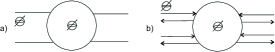
Figure 4: One cell of a Turing machine as a QTA

Again, two automata $T_{i}:(\mathcal{H}_{i},\mathcal{K},\tau_{i})$, $i=1,2$ are called isomorphic if there exists an isometric isomorphism $\sigma:\mathcal{H}_{1}\rightarrow\mathcal{H}_{2}$ for which $\tau_{2}=(\sigma^{\dagger}\otimes I_{\mathcal{K}})\circ\tau_{1}\circ(\sigma\otimes I_{\mathcal{K}})$.

Example.  In Figure 4a, consider the abstract representation of one tape cell drawn from a hypothetical Turing machine having two states: $1$ and $2$. The tape alphabet $\{0,1\}$ is also binary, which means that there is a single qubit sitting in the cell. Thus, $\mathcal{H}$ is 2-dimensional. The control particle $c$ can reside on any of the given four interfaces. For example, if $c$ is on the top left interface, then the control is coming from the left in state 1. After one move, $c$ can again be on any of these four interfaces, so that the dimension of $\mathcal{K}$ is 4. Notice the undirected nature of one move, as opposed to the rigid input$\to$output orientation forced on DQTA. The situation is, however, analogous to having a separate input and dual output interface for each undirected one in a corresponding DQTA. Cf. Figure 4b. The quantum Turing automaton obtained in this way will then have a transition operator $\tau$ as an $8\times 8$ unitary matrix.

Let $\mathcal{C}$ be an arbitrary traced monoidal category. In order to describe the structure of (undirected) quantum Turing automata we shall use a variant of the Joyal-Street-Verity $Int$ construction [18] by which tensor is defined on objects in $Int(\mathcal{C})$ as

$$(X,U)\otimes(X^{\prime},U^{\prime})=(X\otimes_{\mathcal{C}}X^{\prime},U\otimes_{\mathcal{C}}U^{\prime}),$$

and on morphisms $f:(X,U)\rightarrow(Y,V)$, $f^{\prime}:(X^{\prime},U^{\prime})\rightarrow(Y^{\prime},V^{\prime})$ as

$$f\otimes f^{\prime}=(1_{X}\otimes_{\mathcal{C}}c_{X^{\prime},V}\otimes_{\mathcal{C}}1_{V^{\prime}})\circ(f\otimes_{\mathcal{C}}f^{\prime})\circ(1_{Y}\otimes_{\mathcal{C}}c_{U,Y^{\prime}}\otimes_{\mathcal{C}}1_{U^{\prime}}).$$

Recall that $f:X\otimes V\rightarrow Y\otimes U$ in $\mathcal{C}$. Correspondingly,

$$1_{(X,U)}=1_{X\otimes_{\mathcal{C}}U},\;c_{(X,U),(Y,V)}=c_{X,Y}\otimes_{\mathcal{C}}c_{V,U},\mbox{\ and\ }d_{(X,U)}=e_{(X,U)}=(c_{X,U})_{\mathcal{C}}.$$

The reason for the change is that, by the original definition, the self-dual objects $(X,X)$ in $Int(\mathcal{C})$ are not closed for the tensor.

Definition 11.

A CC-category $\mathcal{C}$ is completely symmetric if $A=A^{**}$, $(A\otimes B)^{*}=A^{*}\otimes B^{*}$, and the natural isomorphism $A^{*}\otimes B^{*}\!=\!(A\otimes B)^{*}\cong B^{*}\!\otimes A^{*}$ determined by the duality $()^{*}$ coincides with $c_{A^{*},B^{*}}$ for all objects $A,B$.

In the above definition, “the duality $()^{*}$” refers to the pure autonomous structure of $\mathcal{C}$, forgetting the symmetries. Observe that complete symmetry implies that the coherence conditions in effect for the symmetries $c_{A,B}$ are automatically inherited by the units $d_{A}$ and counits $e_{A}$ in an appropriate way, e.g.,

$$d_{A^{*}}=d_{A}\circ c_{A^{*},A}\mbox{\ \ and\ \ }d_{A\otimes B}=(d_{A}\otimes d_{B})\circ(1_{A}\otimes c_{A,B^{*}}\otimes 1_{B}),$$

as one would normally expect. These equations do not necessarily hold without complete symmetry.

Proposition 12.

For every traced monoidal category $\mathcal{C}$, the CC-category $Int(\mathcal{C})$ is completely symmetric.

Proof. Immediate by the definitions. q.e.d.

Let $Int_{0}(\mathcal{C})$ denote the full subcategory of $Int(\mathcal{C})$ determined by its self-dual objects $(X,X)$. Again, as an immediate consequence of the definitions, $()^{*}$ defines a dagger structure on $Int_{0}(\mathcal{C})$ through which it becomes a dagger compact closed category. Clearly, the dagger (dual) of $f:X\otimes_{\mathcal{C}}Y\rightarrow Y\otimes_{\mathcal{C}}X$ as a morphism $(X,X)\rightarrow(Y,Y)$ is $c_{Y,X}\circ f\circ c_{Y,X}$. In general, we put forward the following definition.

Definition 13.

A completely symmetric self-dual CC category (S²DC² category, for short) is a completely symmetric CC category such that $A=A^{*}$ for all objects $A$.

Corollary 14.

In every S²DC² category $\mathcal{C}$, the contravariant functor $()^{*}$ defines a dagger structure on $\mathcal{C}$ by which it becomes dagger compact closed. Consequently, $d_{A}=d_{A}\circ c_{A,A}$ and $e_{A}=c_{A,A}\circ e_{A}$ hold in $\mathcal{C}$. For every traced monoidal category $\mathcal{C}$, $Int_{0}(\mathcal{C})$ is an S²DC² category.

Proof. Cf. Figure 1. q.e.d.

Now let us assume that $\mathcal{C}$ is a dagger traced monoidal category, that is, $\mathcal{C}$ has a monoidal dagger structure for which

$$\mathrm{Tr}^{U}(f^{\dagger})=(\mathrm{Tr}^{U}f)^{\dagger}\mbox{\ \ for $f:U\otimes A\rightarrow U\otimes B$.}$$

This is definitely the case for the subcategory $\mbox{\bf DQT}_{0}$ of DQT consisting of automata having an isometric isomorphism as their transition operator. Moreover, the map $T\mapsto T\boxplus T^{\dagger}$ is injective in $\mbox{\bf DQT}_{0}$.

Theorem 15.

For every dagger traced monoidal category $\mathcal{C}$, the map $f\mapsto f\otimes f^{\dagger}$ defines a strict dagger-traced-monoidal functor $F_{\mathcal{C}}:\mathcal{C}\rightarrow Int_{0}(\mathcal{C})$ by which $F_{\mathcal{C}}A=(A,A)$ for each object $A$.

Proof. Routine computation, left to the reader. q.e.d.

At this point we have sufficient knowledge to understand the structure and behavior of QTA. Indeed, any such automaton $(\mathcal{H},\mathcal{N},\tau)$ with $\tau:\mathcal{H}\otimes\mathcal{N}\rightarrow\mathcal{H}\otimes\mathcal{N}$ is in fact a morphism $(I,I)\rightarrow(\mathcal{N},\mathcal{N})$ in the S²DC² category $Int_{0}(\mbox{\bf DQT}_{0})$. Using the terminology of [2, Definition 3.2], such a morphism is the name of any appropriate morphism $(\mathcal{K},\mathcal{K})\rightarrow(\mathcal{L},\mathcal{L})$ in $Int_{0}(\mbox{\bf DQT}_{0})$ such that $\mathcal{N}=\mathcal{K}\oplus\mathcal{L}$. The natural isomorphism induced by duality simply collapses these hom-sets into their name hom-set. However, the reader should not be confused by the fact that the name of a morphism $f:(X,X)\rightarrow(Y,Y)$ in $Int_{0}(\mathcal{C})$ — that is, $f:X\otimes Y\rightarrow Y\otimes X$ in $\mathcal{C}$ — is in fact a morphism $X\otimes Y\rightarrow X\otimes Y$ in $\mathcal{C}$, actually $f\circ c_{Y,X}$.

In particular, for every automaton $T:\mathcal{K}\rightarrow\mathcal{L}$ in $\mbox{\bf DQT}_{0}$, the name of $F_{\mbox{{\scriptsize{\bf DQT}}}_{0}}T=T\boxplus T^{\dagger}$ as a morphism $(I,I)\rightarrow(\mathcal{K}\oplus\mathcal{L},\mathcal{K}\oplus\mathcal{L})$ is the QTA of rank $\mathcal{K}\oplus\mathcal{L}$ which reflects the joint behavior of $T$ and its reverse. Of course, however, the whole structure of QTA is a lot richer than simply the image of $\mbox{\bf DQT}_{0}$ under $F_{\mbox{{\scriptsize{\bf DQT}}}_{0}}$. This observation is analogous to the obvious fact that the tensor of two vector spaces is richer than the collection of tensors of individual vectors. Building on this analogy we can consider the collection of QTA as a suitable algebraic structure, rather than a category.

An equivalent formalism for S²DC² categories in terms of so called indexed monoidal algebras has been worked out in [7, 8]. This new formalism deals with QTA as “vectors” rather than morphisms, in the spirit explained in the previous paragraph. The basis of the equivalence between indexed monoidal algebras and S²DC² categories is the naming mechanism, which identifies morphisms with their names. The advantage of using this algebraic framework is that it simplifies the understanding of S²DC² categories by essentially collapsing the dual category structure, which may sometimes be extremely but unnecessarily convoluted.

6 Conclusion

We have provided a theoretical foundation for the study of quantum Turing machines having a quantum control. The dagger compact closed category FdHilb of finite dimensional Hilbert spaces served as the basic underlying structure for this foundation. We narrowed down the scope of this category to isometries, switched from multiplicative to additive tensor, and defined a new additive trace operation by the help of the Moore-Penrose generalized inverse. This trace was then carried over to the monoidal category of directed quantum Turing automata. Finally, we applied the $Int$ construction to obtain a compact closed category, and restricted this category to its self-dual objects to arrive at our ultimate goal, the model (indexed monoidal algebra) of undirected quantum Turing automata.

References

• [1]
• [2] S. Abramsky & B. Coecke (2004): A categorical semantics of quantum protocols. In: 19th IEEE Symposium on Logic in Computer Science (LICS 2004), 14-17 July 2004, Turku, Finland, Proceedings IEEE Computer Society Press, pp. 415–425, 10.1109/LICS.2004.1319636.
• [3] M. Bartha (1987): A finite axiomatization of flowchart schemes. Acta Cybernetica 8, pp. 203–217.
• [4] M. Bartha (1987): An equational axiomatization of systolic systems. Theoretical Computer Science 55, pp. 265–289, 10.1016/0304-3975(87)90104-6.
• [5] M. Bartha (1992): An algebraic model of synchronous systems. Information and Computation 97, pp. 97–131, 10.1016/0890-5401(92)90006-2.
• [6] M. Bartha (2008): Simulation equivalence of automata and circuits. In: E. Csuhaj-Varjú, Z. Ésik (eds.), Automata and Formal Languages, 12th International Conference, AFL 2008, Balatonfüred, Hungary, May 27-30, 2008, Proceedings, pp. 86-99.
• [7] M. Bartha (2010): Turing automata and graph machines. In: S. B. Cooper, P. Panangaden, E. Kashefi (eds.), Proceedings Sixth Workshop on Developments in Computational Models: Causality, Computation, and Physics, Electronic Proceedings in Theoretical Computer Science 26, pp. 19–31, 10.4204/EPTCS.26.3.
• [8] M. Bartha (2013): The monoidal structure of Turing machines. Mathematical Structures in Computer Science 23(2):204-246, 10.1017/S0960129512000096.
• [9] A. Ben-Israel & T.N.E. Greville (2003): Generalized Inverses: Theory and Applications. Springer-Verlag, Berlin.
• [10] D.S. Bernstein (2005): Matrix Mathematics. Princeton University Press, Princeton, NJ.
• [11] S.L. Bloom & Z. Ésik (1993): Iteration Theories: The Equational Logic of Iterative Processes. Springer-Verlag, Berlin.
• [12] J.R.B. Cockett, M. Hasegawa, & R.A.G. Seely (2006): Coherence of the double involution on $*$-autonomous categories. Theory and Application of Categories 17(2), pp. 17–29.
• [13] E. D’Hondt & P. Panangaden (2006): Quantum weakest preconditions. Mathematical Structures in Computer Science 16, pp. 429–451, 10.1017/S0960129506005251.
• [14] L. de Francesco Albasini, N. Sabadini, & R.F.C. Walters (2011): An algebra of automata which includes both classical and quantum entities. Electronic Notes in Theoretical Computer Science 270, pp. 263–272, 10.1016/j.entcs.2011.01.036.
• [15] J.-Y. Girard (1989): Geometry of Interaction I: Interpretation of system F. In: R. Ferro, C. Bonotto, S. Valentini, A. Zanardo (eds.), Logic Colloquium ’88. Proceedings of the colloquium held at the University of Padova, Padova, August 22–31, 1988, Studies in Logic and the Foundations of Mathematics, 127. North-Holland, Amsterdam, pp. 221-260, 10.1016/S0049-237X(08)70271-4.
• [16] E. Haghverdi & P.J. Scott (2010): Towards a typed geometry of interaction. Mathematical Structures in Computer Science 20, pp. 1–49, 10.1017/S096012951000006X.
• [17] I. Hasuo & N. Hoshino (2011): Semantics of higher order quantum computation via Geometry of Interaction. In: Proceedings of the 26th Annual IEEE Symposium on Logic in Computer Science, LICS 2011, June 21-24, 2011, Toronto, Ontario, Canada, IEEE Computer Society Press, pp. 237–246, 10.1109/LICS.2011.26.
• [18] A. Joyal, R. Street, & D. Verity (1996): Traced monoidal categories. Mathematical Proceedings of the Cambridge Philosophical Society 119, pp. 447–468, 10.1017/S0305004100074338.
• [19] P. Katis, N. Sabadini, & R.F.C. Walters (2002): Feedback, trace, and fixed-point semantics. RAIRO Theoretical Informatics and Applications 36, pp. 181–194, 10.1051/ita:2002009.
• [20] G.M. Kelly & M.L. Laplaza (1980): Coherence for compact closed categories. Journal of Pure and Applied Algebra 19, pp. 193–213, 10.1016/0022-4049(80)90101-2.
• [21] S. Mac Lane (1997): Categories for the Working Mathematician, Springer-Verlag, Berlin.
• [22] O. Malherbe, P.J. Scott & P. Selinger (2011): Partially traced categories. Journal of Pure and Applied Algebra 216(12), pp. 2563–2585, 10.1016/j.jpaa.2012.03.026.
• [23] S. Roman (2005): Advanced Linear Algebra, Springer-Verlag, Berlin.
• [24] P. Selinger (2007): Dagger compact closed categories and completely positive maps. Electronic Notes in Theoretical Computer Science 170, pp. 139–163, 10.1016/j.entcs.2006.12.018.
• [25] P. Selinger (2004): Towards a quantum programming language. Mathematical Structures in Computer Science 14, pp. 527–586, 10.1017/S0960129504004256.