On the Complexity of the Constrained Input Selection Problem for Structural Linear Systems

Abstract

This paper studies the problem of, given the structure of a linear-time invariant system and a set of possible inputs, finding the smallest subset of input vectors that ensures system’s structural controllability. We refer to this problem as the minimum constrained input selection (minCIS) problem, since the selection has to be performed on an initial given set of possible inputs. We prove that the minCIS problem is NP-hard, which addresses a recent open question of whether there exist polynomial algorithms (in the size of the system plant matrices) that solve the minCIS problem. To this end, we show that the associated decision problem, to be referred to as the CIS, of determining whether a subset (of a given collection of inputs) with a prescribed cardinality exists that ensures structural controllability, is NP-complete. Further, we explore in detail practically important subclasses of the minCIS obtained by introducing more specific assumptions either on the system dynamics or the input set instances for which systematic solution methods are provided by constructing explicit reductions to well known computational problems. The analytical findings are illustrated through examples in multi-agent leader-follower type control problems.

I Introduction

Research on large-scale control systems has grown considerably over the last few years, triggered by technological advances in sensing and actuation infrastructures and relatively low cost of deployment. Such pervasive sensing and actuation present tremendous opportunities for enhanced system control, although, at the cost of handling and processing enormous amounts of sensor data for system state inference and subsequently coordinating generated control signals among the actuators distributed throughout the system. Thus, it is of importance to understand which subsets of sensors and actuators (hence the smallest amount of data that need to be processed and coordination required) are crucial for achieving desirable system monitoring (observability) and control (controllability) performance. These and related questions form the core of the input/output selection problems [5, 13, 14] in large-scale control systems. In this paper, we focus on the problem of, given a possibly large scale linear-time invariant system and a set of possible inputs, finding the smallest subset of input vectors that ensures system’s controllability. Notice that, by duality between controllability and observability for linear-time invariant systems, another problem can be posed in terms of determining the minimal number of outputs that ensure observability, whose solution is straightforward from knowing how to solve the related controllability problem.

Now, consider the system

$$\dot{x}(t) =Ax(t)+Bu(t)$$ (1)

where $x\in\mathbb{R}^{n}$ is the state, $u\in\mathbb{R}^{p}$ and $y\in\mathbb{R}^{m}$ denote the input and output vectors, respectively. Additionally, let $\bar{A}\in\{0,\star\}^{n\times n}$ denote the zero/nonzero or structural pattern of the system matrix $A$, whereas $\bar{B}\in\{0,\star\}^{n\times p}$ is the structural pattern of the input matrix $B$; more precisely, an entry in these matrices is zero if the corresponding entry in the system matrices is equal to zero, and a free parameter (denoted by a star) otherwise. Notice that the structural matrices defined above determine the coupling between the system state variables, and the state variables actuated by the inputs deployed in the system. The structural matrices are the object of study in structural systems theory [4], where the pair $(\bar{A},\bar{B})$ is said to be structurally controllable if there exists a numerical realization $(A,B)$ in (1) with the same structure, i.e., having zeros in the specified locations, as $(\bar{A},\bar{B})$ that is controllable. In fact, a stronger characterization holds, and it can be shown that the set of non-controllable numerical realizations $(A,B)$ of a structurally controllable pair $(\bar{A},\bar{B})$ has zero Lebesgue measure in the product space $\mathbb{R}^{n\times n}\times\mathbb{R}^{n\times p}$; in other words, almost all numerical realizations of a structurally controllable pair are controllable [4]. Hereafter, we restrict attention to structural system theoretic properties. More specifically, given the structural matrix and possible input configurations, the minimum constrained input selection (minCIS) problem consists of identifying the smallest subset of inputs that ensure structural controllability and may be formally posed as follows

$\mathcal{P}_{1}$ Given $\bar{A}\in\{0,\star\}^{n\times n}$ and $\bar{B}\in\{0,\star\}^{n\times p}$, determine

$$\mathcal{J}^{*}=\arg\min\limits_{\mathcal{J}\subset\{1,\ldots,p\}} \qquad\qquad|\mathcal{J}|$$ (2)

s.t. $$(\bar{A},\bar{B}_{\mathcal{J}})\text{ is structurally controllable,}$$

where $\mathcal{J}$ is a subset of indices associated with the inputs and $\bar{B}_{\mathcal{J}}$ corresponds to the subset of columns in $\bar{B}$ with index in $\mathcal{J}$. $\diamond$

Remark 1

The results that we obtain for the minCIS problem $\mathcal{P}_{1}$ readily extend to the corresponding output selection problem by the duality between observability and controllability in linear systems, and, hence, in what follows, we focus on the minCIS only. In addition, note that the current setup considers continuous time systems, however, all our results apply to the discrete time setting as well due to similar controllability criteria. $\diamond$

Problem $\mathcal{P}_{1}$ has been previously explored by several authors, see [1] and references therein. In fact, [1] provided the motivation for the present paper, in which the following question was posed: Is there a polynomial solution to $\mathcal{P}_{1}$?

In this paper, we address the above question in general scenarios.

In what follows, we use some concepts of computational complexity theory [2], that addresses the classification of (computational) problems into complexity classes. Formally, this classification is for decision problems, i.e., problems with an “yes” or “no” answer. Further, for a decision problem, if there exists a procedure/algorithm that obtains the correct answer in a number of steps that is bounded by a polynomial in the size of the input data to the problem, then the algorithm is referred to as an efficient or polynomial solution to the decision problem and the decision problem is said to be polynomially solvable or belong to the class of polynomially solvable problems. A decision problem is said to be in NP (i.e., the class of nondeterministic polynomially problems) if, given any possible solution instance, it can be verified using a polynomial procedure whether the instance constitutes a solution to the problem or not. It is easy to see that any problem that is polynomially is also in NP, although, there are some problems in NP for which it is unclear whether polynomial solutions exist or not. These latter problems are referred to as being NP-complete. Consequently, the class of NP-complete problems are the hardest among the NP problems, i.e., those that are verifiable using polynomial algorithms, but no polynomial algorithms are known to exist that solve them. Whereas the above classification is intended for decision problems, it can be immediately extended to optimization problems, by noticing that every optimization problem can be posed as a decision problem. More precisely, given a minimization problem, we can pose the following decision problem: Is there a solution to the minimization problem that is less than or equal to a prescribed value? On the other hand, if the solution to the optimization problem is obtained, then any decision version can be easily addressed. Consequently, if a (decision) problem is NP-complete, then the associated optimization problem is referred to as being NP-hard. We refer the reader to [6] for an introduction to the topic, and Section II for further discussion.

In fact, one of the main results of the present paper consists in showing the NP-completeness of the decision version of the minCIS problem, which we refer to as constrained input selection (CIS) problem, and given as follows.

$\mathcal{P}_{1}^{d}$ Is there a collection of indices $\mathcal{J}\subset\{1,\ldots,p\}$ with at most $k$ elements (i.e., $|\mathcal{J}|\leq k$) such that $(\bar{A},\bar{B}_{\mathcal{J}})$ is structurally controllable?

The NP-completeness of CIS is attained by polynomially reducing the set covering problem to it. Hence, in particular, polynomial complexity algorithms that solve general instances of the CIS and minCIS are unlikely to exist. Nevertheless, there could be subclasses of the minCIS that admit polynomial complexity algorithmic solutions, as is the case with a practically relevant subclass of minCIS problems identified in this paper; more precisely, when the input matrix $\bar{B}$ is restricted to be structurally similar to the $n\times n$ identity matrix (but $\bar{A}$ is arbitrary).

In addition, since the CIS is NP-complete, the minCIS may be polynomially reduced to other (more standard) NP-hard problems, through polynomial reductions between their decision versions. Practically, such reduction may lead to efficient (polynomial complexity) approximation schemes for solving the minCIS with guaranteed suboptimality bounds. While we do not provide such reductions from general minCIS instances to other NP-hard problems, for a certain restricted subclass of minCIS problems (with some additional conditions on the dynamic matrix structure) we explicitly construct a reduction to the minimum set covering problem. This reduction builds upon the complexity remarks elaborated in [1], yet it holds for a larger class of instances, and only relies on a condition on the structure of the dynamics. Furthermore, this restricted class is practically relevant and, as shown later, subsumes important applications in multi-agent control such as leader-follower problems [8, 9]; as a demonstration, we show how our reduction can be used to solve the leader-selection problem and a more general variant of it, which we refer to as the constrained leader-selection problem.

The main results of the paper are threefold: (i) we show that CIS is NP-complete, which implies that the minCIS is NP-hard; (ii) we identify a subclass of minCIS problems that are polynomially solvable; more precisely, under the assumption that the input matrix is structurally similar to the identity matrix; and (iii) we provide a polynomial reduction of the minCIS problem to a minimum set covering problem under a mild assumption on the structure of the dynamic matrix (given in Assumption 1), that hold for several interconnected dynamical systems, as well as leader-selection problems like those introduced in Section 4.

The rest of this paper is organized as follows: Section 2 introduces some preliminaries on computational complexity theory, associated complexity classes and polynomial reductions between problems. Additionally, we review some concepts and results in structural systems theory to be used in the sequel. Section 3 presents the result that the CIS is NP-complete, and, subsequently, minCIS is NP-hard. In Section 4, a polynomial reduction from the minCIS to the minimum set covering problem is provided, under certain assumptions on the minCIS instances. Finally, an illustrative example is described in Section 5.

II Preliminaries and Terminology

In this section, we review the minimum set covering problem, and its decision version, referred to as the set covering problem [3]. In addition, some necessary and sufficient conditions that ensure system’s structural controllability, required to obtain the results presented in the paper, are introduced in Section 2.1.

A (computational) problem is said to be reducible in polynomial time to another if there exists a procedure to transform the former to the latter using a polynomial number of operations on the size of its inputs. Such reduction is useful in determining the qualitative complexity class [6] a particular problem belongs to. The following result may be used to check for NP-completeness of a given problem.

Lemma 1 ([6])

If a problem $\mathcal{P}_{A}$ is NP-complete, $\mathcal{P}_{B}$ is in NP and $\mathcal{P}_{A}$ is reducible in polynomial time to $\mathcal{P}_{B}$, then $\mathcal{P}_{B}$ is NP-complete. $\diamond$

Now, consider the set covering (decision) problem: Given a collection of sets $\{\mathcal{S}_{j}\}_{j=1,\ldots,p}$, where $\mathcal{S}_{j}\subset\mathcal{U}$, is there a collection of at most $k$ sets that covers $\mathcal{U}$, i.e., $\bigcup_{j\in\mathcal{K}}\mathcal{S}_{j}=\mathcal{U}$, where $\mathcal{K}\subset\{1,\ldots,p\}$ and $|\mathcal{K}|\leq k$?

This is the decision problem associated with the minimum set covering problem, a well known NP-hard problem, given as follows.

Definition 1 ([3])

(Minimum Set Covering Problem) Given a set of $m$ elements $\,\mathcal{U}=\left\{1,2,\ldots,m\right\}$ and a set of $n$ sets $\mathcal{S}=\left\{\mathcal{S}_{1},\ldots,\mathcal{S}_{n}\right\}$ such that $\mathcal{S}_{i}\subset\mathcal{U}$, with $i\in\{1,\cdots,n\}$, and $\displaystyle\bigcup_{i=1}^{n}\mathcal{S}_{i}=\mathcal{U}$, the minimum set covering problem consists of finding a set of indices $\,\mathcal{I}^{*}\subseteq\left\{1,2,\ldots,n\right\}$ corresponding to the minimum number of sets covering $\mathcal{U}$, i.e.,

$$\begin{array}[]{rl}\mathcal{I}^{*}=\underset{\mathcal{I}\subseteq\left\{1,2,\ldots,n\right\}}{\arg\min}&\quad|\mathcal{I}|\\ \text{s.t. }&\mathcal{U}=\displaystyle\bigcup_{i\in\mathcal{I}}\mathcal{S}_{i}\ .\end{array}$$

$\diamond$

In particular, the set covering problem is used in the present paper to show the NP-completeness of $\mathcal{P}_{1}^{d}$, by considering the following result.

Proposition 1 ([6])

Let $\mathcal{P}_{A}$ and $\mathcal{P}_{B}$ be two optimization problems, and $\mathcal{P}_{B}^{d}$ the decision versions associated with $\mathcal{P}_{B}$. If a problem $\mathcal{P}_{A}$ is NP-hard, an instance of $\mathcal{P}_{B}^{d}$ can be efficiently verified and $\mathcal{P}_{A}$ is polynomially reducible to $\mathcal{P}_{B}$, then $\mathcal{P}_{B}^{d}$ is NP-complete. In particular, $\mathcal{P}_{B}$ is NP-hard. $\diamond$

II-A Structural Systems

Structural systems provide an efficient representation of a linear-time invariant system as a directed graph (digraph). A digraph consists of a set of vertices $\mathcal{V}$ and a set of directed edges $\mathcal{E}_{\mathcal{V},\mathcal{V}}$ of the form $(v_{i},v_{j})$ where $v_{i},v_{j}\in\mathcal{V}$. If a vertex $v$ belongs to the endpoints of an edge $e\in\mathcal{E}_{\mathcal{V},\mathcal{V}}$, we say that the edge $e$ is incident to $v$. We represent the state digraph by $\mathcal{D}(\bar{A})=(\mathcal{X},\mathcal{E}_{\mathcal{X},\mathcal{X}})$, i.e., the digraph that comprises only the state variables as vertices denoted by $\mathcal{X}=\{x_{1},\cdots,x_{n}\}$ and a set of directed edges between the state vertices denoted by $\mathcal{E}_{\mathcal{X},\mathcal{X}}=\left\{(x_{i},x_{j})\in\mathcal{X}\times\mathcal{X}:\ \bar{A}_{j,i}\neq 0\right\}$. Similarly, we represent the system digraph by $\mathcal{D}(\bar{A},\bar{B})=(\mathcal{X}\cup\mathcal{U},\mathcal{E}_{\mathcal{X},\mathcal{X}}\cup\mathcal{E}_{\mathcal{U},\mathcal{X}})$, where $\mathcal{U}=\{u_{1},\cdots,u_{p}\}$ corresponds to the input vertices and $\mathcal{E}_{\mathcal{U},\mathcal{X}}=\left\{(u_{i},x_{j})\in\mathcal{U}\times\mathcal{X}:\ \bar{B}_{i,j}\neq 0\right\}$ the edges identifying which state variables are actuated by which inputs. Further, we say that an input $u_{i}$ is assigned to a state variable $x_{j}$ if $\bar{B}_{i,j}\neq 0$.

A directed path between the vertices $v_{1}$ and $v_{k}$ is a sequence of edges $\{(v_{1},v_{2}),(v_{2},v_{3}),\ldots,$ $(v_{k-1},v_{k})\}$. If all the vertices in a directed path are different, then the path is said to be an elementary path. A cycle is a directed path such that $v_{1}=v_{k}$ and all remaining vertices in the direct path are distinct.

We also require the following graph theoretic notions [3]: A digraph $\mathcal{D}$ is strongly connected if there exists a directed path between any two vertices. A strongly connected component (SCC) is a maximal subgraph $\mathcal{D}_{S}=(\mathcal{V}_{S},\mathcal{E}_{S})$ of $\mathcal{D}$ such that for every $u,v\in\mathcal{V}_{S}$ there exist paths from $u$ to $v$ and from $v$ to $u$.

By visualizing each SCC as a virtual node, we can build a directed acyclic graph (DAG) representation, in which a directed edge exists between vertices belonging to two SCCs if and only if there exists a directed edge connecting the corresponding SCCs in the original digraph $\mathcal{D}=(\mathcal{V},\mathcal{E})$. The construction of the DAG associated with $\mathcal{D}(\bar{A})$ can be performed efficiently in $\mathcal{O}(|\mathcal{V}|+|\mathcal{E}|)$ [3]. In Figure 1, we present a digraph and its DAG representation: by convention, the arrows connecting the different SCCs are facing downwards, which motivates the classification of the SCCs in the DAG as follows.

Definition 2 ([10, 11])

An SCC is said to be linked if it has at least one incoming/outgoing edge from another SCC. In particular, an SCC is non-top linked if it has no incoming edges to its vertices from the vertices of another SCC. $\diamond$

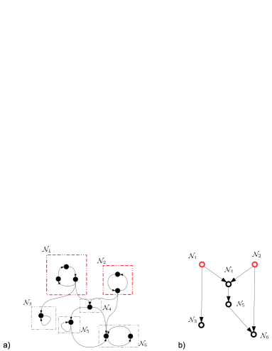
Figure 1: In a) the SCCs are depicted by dashed boxes, labelled by $\mathcal{N}_{i}$ ($i=1,\ldots,6$), and the non-top linked SCCs $\mathcal{N}_{1}$ and $\mathcal{N}_{2}$ are depicted in red. In b), these SCCs correspond to vertices ($\mathcal{N}_{1}$ and $\mathcal{N}_{2}$) in the DAG representation.

Given $\mathcal{D}=(\mathcal{V},\mathcal{E})$, we can construct a bipartite graph $\mathcal{B}(\mathcal{S}_{1},\mathcal{S}_{2},\mathcal{E}_{\mathcal{S}_{1},\mathcal{S}_{2}})$, where $\mathcal{S}_{1},\mathcal{S}_{2}\subset\mathcal{V}$ and the edge set $\mathcal{E}_{\mathcal{S}_{1},\mathcal{S}_{2}}=\{(s_{1},s_{2})\in\mathcal{E}\ :\ s_{1}\in\mathcal{S}_{1},s_{2}\in\mathcal{S}_{2}\ \}.$ Such bipartite graphs will be used throughout in connection with the minCIS and we provide some elementary concepts associated with bipartite graphs. Given $\mathcal{B}(\mathcal{S}_{1},\mathcal{S}_{2},\mathcal{E}_{\mathcal{S}_{1},\mathcal{S}_{2}})$, a matching $M$ corresponds to a subset of edges in $\mathcal{E}_{\mathcal{S}_{1},\mathcal{S}_{2}}$ that do not share vertices, i.e., given edges $e=(s_{1},s_{2})$ and $e^{\prime}=(s_{1}^{\prime},s_{2}^{\prime})$ with $s_{1},s_{1}^{\prime}\in\mathcal{S}_{1}$ and $s_{2},s_{2}^{\prime}\in\mathcal{S}_{2}$, $e,e^{\prime}\in M$ only if $s_{1}\neq s_{1}^{\prime}$ and $s_{2}\neq s_{2}^{\prime}$. A maximum matching $M^{\ast}$ is a matching $M$ with the largest number of edges among all possible matchings. Note that, in general, a maximum matching may not be unique. A maximum matching can be computed efficiently in $\mathcal{O}(\sqrt{|\mathcal{S}_{1}\cup\mathcal{S}_{2}|}|\mathcal{E}_{\mathcal{S}_{1},\mathcal{S}_{2}}|)$ using, for instance, the Hopcroft-Karp algorithm [3].

Given a matching $M$, an edge is said to be matched with respect to (w.r.t.) $M$, if it belongs to $M$. In addition, we say that a vertex $\,v\in\mathcal{V}_{1}\cup\mathcal{V}_{2}\,$ is matched if it is incident to some matched edge in $M$, otherwise we say that the vertex is free w.r.t. $M$. Incident and free vertices can be further characterized as follows: a vertex in $\mathcal{S}_{2}$ is a right-matched vertex if it is incident to an edge in $M^{\ast}$, otherwise, it is an right-unmatched vertex. A maximum matching in which there are no free vertices (or equivalently, either left/right-unmatched vertices) is called a perfect matching.

Given a state digraph $\mathcal{D}(\bar{A})=(\mathcal{X},\mathcal{E}_{\mathcal{X},\mathcal{X}})$, a particular bipartite graph of interest is its bipartite representation denoted as $\mathcal{B}(\bar{A})\equiv\mathcal{B}(\mathcal{X},\mathcal{X},\mathcal{E}_{\mathcal{X},\mathcal{X}})$, and we refer to it as the state bipartite graph. The state bipartite graph may be used to characterize all possible structurally controllable pairs $(\bar{A},\bar{B})$, see [10]. In particular, in the sequel, we will use the following result.

Proposition 2 ([10, 11])

Given $\mathcal{D}(\bar{A})=(\mathcal{X},\mathcal{E}_{\mathcal{X},\mathcal{X}})$ and its DAG representation, constituted by $k$ SCCs, denoted by $\{\mathcal{N}_{i}\}_{i=1}^{k}$, where $\mathcal{N}_{i}=(\mathcal{X}_{i},\mathcal{E}_{\mathcal{X}_{i},\mathcal{X}_{i}})$, let $\mathcal{N}_{i_{1}},\ldots\mathcal{N}_{i_{m}}$ be the non-top linked SCCs in the DAG representation with $\{i_{1},\ldots,i_{m}\}\subset\{1,\ldots,k\}$ and $\mathcal{B}(\bar{A})$ the state bipartite graph. If $\mathcal{B}(\bar{A})$ has a perfect matching, then $(\bar{A},\bar{B})$ is structurally controllable if and only if for each non-top linked SCC there exists an input (corresponding to a column in $\bar{B}$) assigned to, i.e., connected to, at least one of its state variables. $\square$

III Main Results

In this section, we show that the minCIS presented in $\mathcal{P}_{1}$ is NP-hard (Corollary 1), by showing that its decision version, the CIS, is an NP-complete problem (Theorem 1). Then, we identify a subclass of minCIS problems that are polynomially solvable (Theorem 2).

We start by showing that CIS is NP-complete, as provided in the following result.

Theorem 1

The constrained input selection (CIS) problem presented in $\mathcal{P}_{1}^{d}$ is NP-complete.

$\diamond$

Proof:

The proof follows by using Proposition 1; more precisely, by presenting the polynomial reduction from the minimum set covering problem to minCIS, and noticing that $\mathcal{P}_{1}^{d}$ is in NP, i.e., there exist polynomial algorithms to verify if $(\bar{A},\bar{B}(\mathcal{J}))$, for some $\mathcal{J}\subset\{1,\ldots,p\}$, is structurally controllable [1].

To obtain the polynomial reduction, consider a general minimum set covering problem instance with sets $\{\mathcal{S}_{i}\}_{i\in\mathcal{I}}$, the index set $\mathcal{I}=\{1,\ldots,p\}$ and universe $\mathcal{U}=\bigcup\limits_{i\in\mathcal{I}}\mathcal{S}_{i}$, where $|\mathcal{U}|=n$. Subsequently, construct $\bar{A}\in\{0,\star\}^{n\times n}$ to be a diagonal matrix with nonzero entries, i.e., $\star$, in its diagonal. Additionally, select $\bar{B}\in\{0,\star\}^{n\times p}$, such that its $(i^{\prime},j^{\prime})$-th entry is given as follows:

$$\bar{B}_{i^{\prime},j^{\prime}}=\left\{\begin{array}[]{cc}\star,&\ \text{ if }i^{\prime}\in\mathcal{S}_{j^{\prime}}\\ 0,&\text{ otherwise,}\end{array}\right.$$

for $i^{\prime}\in\{1,\ldots,n\}$ and $j^{\prime}\in\{1,\ldots,p\}$.

Note that such $\mathcal{D}(\bar{A})=(\mathcal{X},\mathcal{E}_{\mathcal{X},\mathcal{X}})$, consists of $n$ non-top linked SCCs and the associated state bipartite graph $\mathcal{B}(\bar{A})$ has a perfect matching. Now, recall that, by Proposition 2, $(\bar{A},\bar{B}(\mathcal{J}))$, for some $\mathcal{J}\subset\{1,\ldots,n\}$, is structurally controllable if and only if each non-top linked SCC of $\mathcal{D}(\bar{A})$ contains a state variable that is connected from an input (corresponding to a nonzero column in $\bar{B}(\mathcal{J})$).

Subsequently, we first show that a feasible solution to the minCIS leads to a feasible solution of the minimum set covering problem, and secondly, a (minimal) solution to the minCIS leads to a (minimal) solution of the minimum set covering problem. To show feasibility, let $\bar{B}(\mathcal{J})$, for some $\mathcal{J}$, be a feasible solution to the minCIS, i.e., $(\bar{A},\bar{B}(\mathcal{J}))$ is structurally controllable. It then follows that there exists edges from the inputs associated with indices in $\mathcal{J}$ to all the state variables (corresponding to the non-top linked SCCs in $\mathcal{D}(\bar{A})$), which implies by the construction of $\bar{B}$ that the family of subsets $\{\mathcal{S}_{j}\}_{j\in\mathcal{J}}$ cover $\mathcal{U}$.

To obtain minimality, suppose, on the contrary, that $\mathcal{J}^{\ast}$ constitutes a (minimal) solution to the minCIS, but the family $\{\mathcal{S}_{j}\}_{j\in\mathcal{J}^{\ast}}$ is not a minimum covering of $\mathcal{U}$. Then, there exists $\mathcal{J}^{\prime}\subset\{1,\ldots,p\}$ with $|\mathcal{J}^{\prime}|<|\mathcal{J}^{*}|$ such that the family $\{\mathcal{S}_{j}\}_{j\in\mathcal{J}^{\prime}}$ covers $\mathcal{U}$. This, in turn, by the construction of $\bar{B}$ and Proposition 2 implies that the pair $(\bar{A},\bar{B}(\mathcal{J}^{\prime}))$ is structurally controllable. Since $|\mathcal{J}^{\prime}|<|\mathcal{J}^{*}|$, we conclude that $\bar{B}(\mathcal{J}^{*})$ is not a (minimal) solution to the minCIS, which is a contradiction. ∎

From Theorem 1, we obtain one of the main results of this paper.

Corollary 1

The minimum constrained input selection (minCIS) problem is NP-hard. $\diamond$

The fact that the minCIS is NP-hard, however, does not rule out the possibility that there exist subclasses of the minCIS (with restricted input instances) that admit polynomial complexity algorithmic solutions (in the size of the system plant matrices). In fact, a particularly interesting subclass of the minCIS is one in which the collection of inputs initially given consist of all possible dedicated inputs, i.e., the matrix $\bar{B}$ consists of $n$ inputs each of which is assigned to a single distinct state variable. Formally, we have the following result.

Theorem 2

Let $\bar{A}\in\{0,\star\}^{n\times n}$ be a given structural dynamic matrix and $\bar{B}=\mathbb{I}_{n}\$ a $\ n\times n$ diagonal input matrix with nonzero diagonal entries. The problem of determining $\mathcal{J}^{*}$ such that

$$\mathcal{J}^{*}=\arg\min\limits_{\mathcal{J}\subset\{1,\ldots,N\}} \qquad\qquad|\mathcal{J}|$$ (3)

$$\text{s.t. }\quad(\bar{A}, \mathbb{I}_{n}(\mathcal{J}))\text{ is structurally controllable,}$$

where $\mathbb{I}_{n}(\mathcal{J})$ corresponds to the columns of $\mathbb{I}_{n}$ with indices in $\mathcal{J}$, referred to as the minimum dedicated input selection problem, can be solved polynomially. More precisely, in $\mathcal{O}(n^{3})$. $\diamond$

Proof:

See Appendix. ∎

In Theorem 2, upon a restriction in $\bar{B}$, we obtained a subclass of minCIS problems that can be solved polynomially. Next, we impose some restrictions in $\bar{A}$, and we show that the problem can be systematically solved by resorting to a minimum set covering problem.

IV Partial Polynomial Reduction of the minCIS to the Minimum Set Covering Problem

In Section 3 we have showed that $\mathcal{P}_{1}^{d}$ is an NP-complete problem without explicitly deriving a polynomial reduction from $\mathcal{P}_{1}^{d}$ to an NP-complete problem, or equivalently, without explicitly deriving a polynomial reduction from minCIS to another (standard or known) NP-hard problem. In this section, we provide a partial polynomial reduction from the minCIS to the minimum set covering problem (see Theorem 3 below). By partial reduction we mean that it is only valid if the state digraph satisfies certain additional properties, to be made precise in Assumption 1. Notably, the set of state digraphs satisfying Assumption 1 for which the proposed reduction holds, include dynamical systems commonly encountered in multi-agent networked control applications (see Section 4.1 for details). Further, in Section 4.2 we show how the polynomial reduction obtained in Section 4.1 can be used to solve leader-selection problems in multi-agent networks.

Throughout this section, we assume that the system dynamic matrices, i.e., the $\bar{A}$ matrices in the minCIS, satisfy the following condition.

Assumption 1 The structural dynamic matrix $\bar{A}$ is such that the state bipartite graph $\mathcal{B}(\bar{A})=\mathcal{B}(\mathcal{X},\mathcal{X},\mathcal{E}_{\mathcal{X},\mathcal{X}})$ associated with $\bar{A}$, has a perfect matching. In other words, the set of right-unmatched vertices associated with any maximum matching of $\mathcal{B}(\bar{A})$ is empty. $\diamond$

Remark 2 ([10, 11])

In fact, Assumption 1 can be interpreted in terms of the state digraph as follows: the state bipartite graph $\mathcal{B}(\bar{A})$ has a perfect matching if and only if $\mathcal{D}(\bar{A})$ is spanned by a disjoint union of cycles, or, alternatively, it corresponds to a structural matrix such that almost all of its numerical instances are full rank. $\diamond$

We now provide a polynomial reduction from the minCIS to the minimum set covering problem under Assumption 1.

Theorem 3

Consider the minCIS problem with system matrix instance $\bar{A}\in\{0,\star\}^{n\times n}$ and input matrix $\bar{B}\in\{0,\star\}^{n\times p}$, where $\bar{A}$ satisfies Assumption 1. Denote by $\mathcal{N}^{i}$, $i=1,\ldots,k$, the $k$ non-top linked SCCs of $\ \mathcal{D}(\bar{A})$. The minCIS problem can then be polynomially reduced to the minimum set covering problem with universe $\mathcal{U}=\{1,\ldots,k\}$ and sets $\{\mathcal{S}_{j}\}_{j=1,\ldots,p}$, where $\mathcal{S}_{j}=\{i\in\mathcal{U}:\ \bar{B}_{r,j}=\star,\ x_{r}\in\mathcal{N}^{i}\}$. $\diamond$

Proof:

The proof requires two steps: 1) to show that the stated reduction to the set covering problem can be achieved by performing a polynomial number of operations with respect to the size of $\bar{A}$ and $\bar{B}$; and 2) to prove the correctness of the reduction, i.e., to show that, under Assumption 1, the solution to the minCIS can be readily determined from the minimal solution of the set covering problem.

The proposed reduction is polynomial since the non-top linked SCCs of $\mathcal{D}(\bar{A})$ can be determined polynomially, for instance, by computing the DAG associated with $\mathcal{D}(\bar{A})$ (see Section 2.1). Subsequently, the sets $\mathcal{S}_{j}$ and the universe $\mathcal{U}$, constituting the minimum set covering problem, can be constructed with linear complexity in the number of state variables in $\mathcal{D}(\bar{A})$.

To show correctness, suppose, on the contrary, we have $\mathcal{J}^{*}\subset\{1,\ldots,p\}$ such that $\{\mathcal{S}_{j}\}_{j\in\mathcal{J}^{\ast}}$ is a (minimal) solution to the minimum set covering problem, and $B(\mathcal{J}^{*})$ is not a (minimal) solution to the minCIS. Hence, there exists $\mathcal{J}^{-}\subset\{1,\ldots,p\}$, with $|\mathcal{J}^{-}|<|\mathcal{J}^{*}|$, such that $\bar{B}(\mathcal{J}^{-})$ is a solution to minCIS. Now note that since $\bar{A}$ satisfies Assumption 1, the bipartite graph $\mathcal{B}(\bar{A})$ consists of a perfect matching, and hence, by Proposition 2, for each non-top linked SCC $\mathcal{N}^{i}$ of $\mathcal{D}(\bar{A})$, there exists an input corresponding to an index in $\mathcal{J}^{-}$ that is assigned to a state variable in $\mathcal{N}^{i}$.

Thus, by construction of the minimum set covering problem, the family $\{\mathcal{S}_{l}\}_{l\in\mathcal{J}^{-}}$ covers $\mathcal{U}=\{1,\ldots,k\}$. Since $|\mathcal{J}^{-}|<|\mathcal{J}^{*}|$, it follows that the family $\{\mathcal{S}_{j}\}_{j\in\mathcal{J}^{\ast}}$ is not a minimal set covering of $\mathcal{U}$, a contradiction. ∎

In the next section, we introduce a class of multi-agent networked control problems, referred to as leader-selection problems. Further, we explain how the reduction obtained in Theorem 3 can be used to solve these leader-selection problems.

V Illustrative Example

To illustrate the results established in Section 4, we introduce two (structural) variants of leader-selection problems stated in [12], namely, (i) the structural (unconstrained) leader-selection, and (ii) the structural constrained leader-selection, as presented next in $\bar{\mathcal{L}}_{1}$ and $\bar{\mathcal{L}}_{2}$ respectively. We will also show that although the proposed method to solve both problems requires the solution of a set covering problem, problem $\bar{\mathcal{L}}_{1}$ is considerably easier to solve than $\bar{\mathcal{L}}_{2}$; more precisely, although the set covering problem is in general dificult to solve, the class of problems in $\bar{\mathcal{L}}_{1}$ and the associated instances of the minimum set covering problems can be solved by resorting to polynomial algorithms.

The structural (unconstrained) leader-selection problem can be posed as follows: Consider a multi-agent network consisting of $N$ agents, where each agent $i$ has the ability to transmit scalar data to its neighbors and perform updates given by a linear combination of the states it receives as well its own. Let $\bar{W}\in\{0,\star\}^{N\times N}$ denote the sparsity induced by such linear combination rules, and $\mathbb{I}_{N}=\text{diag}(\star,\ldots,\star)\in\{0,\star\}^{N\times N}$ a structural pattern of a diagonal matrix without zeros on it; further, we assume that $\bar{W}$ has nonzero diagonal entries. In addition, let each agent be equipped with an input that only actuates directly its own state, i.e., a dedicated input, which can be represented by letting the input matrix to be $\mathbb{I}_{N}$. The structural (unconstrained) leader-selection problem aims to determining the minimum collection of agents that are required to use their inputs to ensure structural controllability. Formally, we have the following problem:

$\bar{\mathcal{L}}_{1}$ Determine $\mathcal{J}^{*}$ where

$$\mathcal{J}^{*}=\arg\min\limits_{\mathcal{J}\subset\{1,\ldots,N\}} \qquad\qquad|\mathcal{J}|$$ (4)

$$\text{s.t. }(\bar{W} ,\mathbb{I}_{N}(\mathcal{J}))\text{ is structurally controllable. }$$

Alternatively, in the structural (constrained) leader-selection problem, we can consider similar dynamics structure $\bar{W}^{\prime}\in\{0,\star\}^{N\times N}$ (assumed with non-zero diagonal entries), but instead of considering that each agent is equipped with a dedicated input, we assume that they receive input signals from external entities. These entities, can be understood as leaders labelled as $\mathcal{L}=\{1,\cdots,L\}$, corresponding to the set of $L$ potential leaders whose goal is to control the collection of $N$ followers, in this case the agents. Furthermore, denote by $\bar{B}\in\mathbb{R}^{N\times L}\in\{0,\star\}$ the structure of the input matrix representing the actuation exercised by the potential leader agents, i.e., the entry $B_{f,l}$ indicates how leader $l\in\mathcal{L}$ actuates the follower $f\in\{1,\cdots,N\}$. Finally, given a subset $\mathcal{J}\subset\mathcal{L}$, $\bar{B}(\mathcal{J})$ denotes the collection of columns in $\bar{B}$ corresponding to indices in $\mathcal{J}$. The structural (constrained) leader-selection problem can be posed as follows:

$\bar{\mathcal{L}}_{2}$ Determine $\mathcal{J}^{*}$ where

$$\mathcal{J}^{*}=\arg\min\limits_{\mathcal{J}\subset\mathcal{L}} \qquad\qquad\qquad|\mathcal{J}|$$ (5)

s.t. $$(\bar{W}^{\prime},\bar{B}(\mathcal{J}))\text{ is structurally controllable. }$$

We now show that $\bar{\mathcal{L}}_{1},\bar{\mathcal{L}}_{2}$ can be solved using set covering problems by employing the reduction developed in Theorem 3.

Proposition 3

The structural dynamics matrices $\bar{W},\bar{W}^{\prime}\in\{0,\star\}^{N\times N}$ associated with the leader-selection problems $\bar{\mathcal{L}}_{1}$, $\bar{\mathcal{L}}_{2}$ satisfy Assumption 1. $\diamond$

Proof:

Let $\bar{A}\in\{0,\star\}^{N\times N}$ denote the structural matrix $\bar{W}$ or $\bar{W}^{\prime}$ (depending on which problem we consider). The proof follows by noticing that $\mathcal{D}(\bar{A})$ consists of self-loops on all the state vertices, corresponding to the nonzero diagonal entries in $\bar{A}$. Consequently, the matching $M^{*}=\{(x_{i},x_{i})$, $i=1,\ldots,n\}$ is a maximum matching associated with the state bipartite graph $\mathcal{B}(\bar{A})$, which is a perfect matching. In other words, the set of right-unmatched vertices of $\mathcal{B}(\bar{A})$ is empty, and hence Assumption 1 holds. ∎

Because Assumption 1 holds for the problems $\bar{\mathcal{L}}_{1}$ and $\bar{\mathcal{L}}_{2}$, by invoking Theorem 3, it follows that we can solve the structural leader-selection problems using a minimum set covering problem.

Corollary 2

The problems $\bar{\mathcal{L}}_{1},\bar{\mathcal{L}}_{2}$ can be polynomially reduced to minimum set covering problems as given in Theorem 3. $\diamond$

Now, consider the system state digraphs depicted in Figure 2. The agent states are depicted by black vertices (labeled as $x_{i}$, $i=1,\ldots,9$), and the inter-agent dynamical coupling by the black directed edges. Furthermore, consider potential input vertices depicted by blue vertices (labeled as $u_{i}$, $i=1,\ldots,4$), where we have the following two cases: in Figure 2 a) we pose the structural unconstrained leader-selection problem, whereas, in Figure 2 b) , we consider a structural constrained leader-selection problem, in which the blue directed edges (from the inputs to the agents’ states) represent which leaders can actuate which agents.

Hereafter, we illustrate how, both the structural leader-selection problems can be solved using the polynomial reduction developed in Theorem 3 (see also Corollary 3).

Structural (Unconstrained) Leader Selection Problem

The goal is to solve the leader-selection problem $\bar{\mathcal{L}}_{1}$ as formulated in (4) with the structure of the dynamics matrix induced by the state digraph represented by the black vertices and edges as depicted in Figure 2 a). To this end, note that, by Proposition 1 and Corollary 3, $\bar{\mathcal{L}}_{1}$ can be reduced to a set covering problem (see Theorem 3). From Theorem 3, to set up the set covering problem, we obtain $\mathcal{S}_{l}=\emptyset$ for $l\in\{1,\ldots,9\}$ since none of the (potential) inputs $u_{1},\ldots,u_{9}$, i.e. the dedicated inputs assigned to agents 1 to 9 respectively, are assigned to variables in non-top linked SCCs. In addition, $\mathcal{S}_{10}=\{1\}$, $\mathcal{S}_{11}=\{2\}$, $\mathcal{S}_{12}=\{3\}$, $\mathcal{S}_{13}=\{4\}$ , where each set comprises the index of the non-top linked SCC it belongs to, and subsequently the universe $\mathcal{U}=\{1,2,3,4\}$. It is readily seen that the solution to the set covering problem is unique and comprises the sets $\mathcal{S}_{l^{\prime}}$, with $l^{\prime}\in\{10,11,12,13\}$. Hence, from the viewpoint of leader-selection, agents 10 to 13 should be designated as leaders, which uniquely solves the leader-selection problem. Thus, an input must be assigned to the state variables $x_{l^{\prime}}$ ($l^{\prime}\in\{10,11,12,13\}$), as depicted in Figure 2 a) by the blue vertices. It is important to note that in general the set covering problems resulting from structural unconstrained leader-selection problems have the characteristic that the sets $\mathcal{S}_{l}$’s comprise at most a single state variable. It is readily seen that such instances of the set covering problem may be solved using polynomial complexity algorithms (recall the set covering problem is NP-complete in general); in fact, to cover the universe, we only need to consider a set for each of the elements in the universe. This is in accordance with the fact that (3) can be solved using a polynomial complexity algorithm (see Theorem 2).

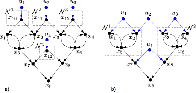
Figure 2: The non-top linked SCCs are depicted by gray dashed boxes and all agents have self-loops (not drawn to keep the illustration simple). In a) we depict the inter-agent communication graph (the agents are depicted by black vertices with associated states as labels) given by the black edges. In addition potential leaders (the vertices $u_{1},u_{2},u_{3}$ depicted in blue) are shown to which a dedicated input may be assigned. Alternatively, in b) we depict a communication graph and possible locations for leaders (the vertices $u_{1},u_{2},u_{3}$ depicted in blue).

Structural Constrained Leader Selection Problem

Now consider the constrained leader-selection problem $\bar{\mathcal{L}}_{2}$ as formulated in (5), with the state digraph induced by the structural dynamics matrix given by the black vertices and edges as depicted in Figure 2 b) and the set of potential leaders depicted by the blue vertices. Additionally, the set of followers actuated by the potential leaders is depicted by the blue edges, i.e., $\bar{B}\in\{0,\star\}^{9\times 4}$ with all entries equal to zero except: $\bar{B}_{1,1}=\bar{B}_{2,1}=\star$ corresponding to input $u_{1}$ assigned to state variables $x_{1}$ and $x_{2}$ respectively and, similarly, $\bar{B}_{2,2}=\bar{B}_{3,2}=\star$, $\bar{B}_{3,3}=\bar{B}_{4,3}=\star$, $\bar{B}_{7,4}=\bar{B}_{8,4}=\star$. Now note that, by Proposition 1 and Corollary 3, $\bar{\mathcal{L}}_{2}$ can be reduced to a set covering problem (see Theorem 3). From Theorem 3, to set up the set covering problem, we obtain $\mathcal{S}_{1}=\{1\}$, $\mathcal{S}_{2}=\{1,2\}$, $\mathcal{S}_{3}=\{2\}$ and $\mathcal{S}_{4}=\emptyset$. In other words, agent 1 can only actuate followers from the non-top linked SCC $\mathcal{N}^{1}$, agent 2 can actuate followers from the non-top linked SCCs $\mathcal{N}^{1},\mathcal{N}^{2}$ and so on. Additionally, the universe is $\mathcal{U}=\{1,2\}$ and in this particular example (note that in general the minimum set covering problem is NP-hard), it is straightforward to see that the solution of the set covering problem consists of the set $\mathcal{S}_{2}$ only. Thus agent 2 should be designated as the leader, which is the solution to the structural constrained leader-selection problem.

VI Conclusions and Further Research

In this paper, we have showed that the decision version of the minimum constrained input selection (minCIS) problem is NP-complete; hence, the minCIS is NP-hard. Consequently, in general, efficient (polynomial complexity) solution procedures to the minCIS are unlikely to exist. Nevertheless, we have identified one subclass of problems, of interest for control systems applications, where the minCIS is efficiently solvable, namely, minCIS instances with dedicated inputs, which can be solved polynomially. The NP-completeness of the decision version of the minCIS further implies that it is polynomially reducible to other NP-complete problems. Subsequently, for a restricted subclass of minCIS problems, which subsumes practically relevant multi-agent networked control applications such as leader-selection problems, we have explicitly constructed a polynomial reduction from the minCIS to the minimum set covering problem. As future research, it may be worthwhile to obtain reductions from more general instances of the minCIS to other standard NP-hard problems, notably the ones with good approximation guarantees, such as the MAX-SAT – the optimization version of the SAT problem [6].

Appendix

To prove Theorem 2, we first introduce and review some of the results presented in [10, 11]. More precisely, consider the minimal structural controllability problem stated as follows: Given $\bar{A}\in\{0,\star\}^{n\times n}$, determine $\bar{B}^{*}$ such that

$$\bar{B}^{*}=\arg\min\limits_{\bar{B}^{*}\in\{0,\star\}^{n\times n}} \qquad\qquad\|\bar{B}\|_{0}$$ (6)

s.t. $$(\bar{A},\bar{B})\text{ is structurally controllable }$$

$$\|\bar{B}_{.,j}\|_{0}\leq 1,\quad j=1,\ldots,n,$$

where $\bar{B}_{.,j}$ corresponds to the $j$-th columns of $\bar{B}$ and $\|M\|_{0}$ counts the number of nonzero entries in the matrix $M\in\{0,\star\}^{n_{1}\times n_{2}}$.

The problem (6) (in fact, a more general variant of (6)) was shown to be polynomially solvable in [10, 11], from which we readily conclude that the minimum dedicated input selection (and output selection, by duality) is polynomially solvable. Further, we note that the sparsity minimization objective (as in (6)) is not generally equivalent to the minCIS, which is consistent with the fact that the minCIS general instance is NP-hard, whereas, the sparsest input/output design problems addressed in [10] are polynomially solvable. Nevertheless, we can use (6) to prove Theorem 2 as follows.

Proof of Theorem 2: The proof follows by noticing that a solution to (6), is of the form $\bar{B}^{*}=[\mathbb{I_{n}^{\mathcal{J}}}\ \mathbf{0}_{n\times(n-|\mathcal{J}|)}]$ (up to permutation), where $\mathbb{I}_{n}^{\mathcal{J}}$ corresponds to the columns of $\mathbb{I}_{n}$ with indices in $\mathcal{J}$, and $\mathbf{0}_{n\times(n-|\mathcal{J}|)}$ is the $n\times(n-|\mathcal{J}|)$ matrix of zeros. Further, we have that $\|\bar{B}^{*}\|_{0}=|\mathcal{J}|$, and since $\bar{B}^{*}$ is a solution to (6), it follows that $|\mathcal{J}|$ is minimum. Consequently, $(\bar{A},\mathbb{I}_{n}^{\mathcal{J}})$ in (6) is structurally controllable, and it readily follows that $(\bar{A},\mathbb{I}_{n}(\mathcal{J}))$ in (3) is structurally controllable. Because, by definition, $\mathbb{I}_{n}^{\mathcal{J}}$ in (6) is the same as $\mathbb{I}_{n}(\mathcal{J})$ in (3), the minimality in the latter holds. Hence, from a minimal solution to (6), it is possible to retrieve a minimal solution to (3).

References

- [1] Christian Commault and Jean-Michel Dion. Input addition and leader selection for the controllability of graph-based systems. Automatica, 49(11):3322–3328, 2013.
- [2] Stephen A. Cook. The complexity of theorem-proving procedures. In Proceedings of the third annual ACM symposium on Theory of computing, STOC ’71, pages 151–158, New York, NY, USA, 1971. ACM.
- [3] Thomas H. Cormen, Clifford Stein, Ronald L. Rivest, and Charles E. Leiserson. Introduction to Algorithms. McGraw-Hill Higher Education, 2nd edition, 2001.
- [4] Jean-Michel Dion, Christian Commault, and Jacob Van der Woude. Generic properties and control of linear structured systems: a survey. Automatica, pages 1125–1144, 2003.
- [5] Magnus Egerstedt. Complex networks: Degrees of control. Nature, 473(7346):158–159, May 2011.
- [6] Michael R. Garey and David S. Johnson. Computers and Intractability: A Guide to the Theory of NP-Completeness. W. H. Freeman & Co., New York, NY, USA, 1979.
- [7] M.D. Ilic, L. Xie, U.A. Khan, and J.M.F. Moura. Modeling of future cyber physical energy systems for distributed sensing and control. IEEE Transactions onSystems, Man and Cybernetics, Part A: Systems and Humans, 40(4):825 –838, July 2010.
- [8] Mehran Mesbahi and Magnus Egerstedt. Graph theoretic methods in multiagent networks. Princeton University Press, 2010.
- [9] Reza Olfati-Saber, J. Alex Fax, and Richard M. Murray. Consensus and Cooperation in Networked Multi-Agent Systems. Proceedings of the IEEE, 95(1):215–233, January 2007.
- [10] S. Pequito, S. Kar, and A. P. Aguiar. A framework for structural input/output and control configuration selection of large-scale systems. Submitted to IEEE Trans. on Automatic Control, Available in http://arxiv.org/abs/1309.5868, 2013.
- [11] S. Pequito, S. Kar, and AP. Aguiar. A structured systems approach for optimal actuator-sensor placement in linear time-invariant systems. In American Control Conference (ACC), 2013, pages 6108–6113, June 2013.
- [12] Amirreza Rahmani, Meng Ji, Mehran Mesbahi, and Magnus Egerstedt. Controllability of multi-agent systems from a graph-theoretic perspective. SIAM J. Control Optim., 48(1):162–186, February 2009.
- [13] Dragoslav D. Siljak. Large-Scale Dynamic Systems: Stability and Structure. Dover Publications, 2007.
- [14] Sigurd Skogestad. Control structure design for complete chemical plants. Computers and Chemical Engineering, 28(1-2):219–234, 2004.