Intermediate Sums on Polyhedra II: Bidegree and Poisson formula

Abstract.

We continue our study of intermediate sums over polyhedra, interpolating between integrals and discrete sums, which were introduced by A. Barvinok [Computing the Ehrhart quasi-polynomial of a rational simplex, Math. Comp. 75 (2006), 1449–1466]. By well-known decompositions, it is sufficient to consider the case of affine cones $s+{\mathfrak{c}}$, where $s$ is an arbitrary real vertex and ${\mathfrak{c}}$ is a rational polyhedral cone. For a given rational subspace $L$, we integrate a given polynomial function $h$ over all lattice slices of the affine cone $s+{\mathfrak{c}}$ parallel to the subspace $L$ and sum up the integrals. We study these intermediate sums by means of the intermediate generating functions $S^{L}(s+{\mathfrak{c}})(\xi)$, and expose the bidegree structure in parameters $s$ and $\xi$, which was implicitly used in the algorithms in our papers [Computation of the highest coefficients of weighted Ehrhart quasi-polynomials of rational polyhedra, Found. Comput. Math.  12 (2012), 435–469] and [Intermediate sums on polyhedra: Computation and real Ehrhart theory, Mathematika 59 (2013), 1–22]. The bidegree structure is key to a new proof for the Baldoni–Berline–Vergne approximation theorem for discrete generating functions [Local Euler–Maclaurin expansion of Barvinok valuations and Ehrhart coefficients of rational polytopes, Contemp. Math. 452 (2008), 15–33], using the Fourier analysis with respect to the parameter $s$ and a continuity argument. Our study also enables a forthcoming paper, in which we study intermediate sums over multi-parameter families of polytopes.

1. Introduction

Let ${\mathfrak{p}}$ be a rational polytope in $V={\mathbb{R}}^{d}$. Computing the volume of the polytope ${\mathfrak{p}}$ and counting the integer points in ${\mathfrak{p}}$ are two fundamental problems in computational mathematics, both of which have a multitude of applications. The same is true for weighted versions of these problems. Let $h(x)$ be a polynomial function on $V$. Then we consider the problems to compute the integral

$$I({\mathfrak{p}},h)=\int_{\mathfrak{p}}h(x)\,\mathrm{d}x$$

and the sum of values of $h(x)$ over the set of integer points of ${\mathfrak{p}}$,

$$S({\mathfrak{p}},h)=\sum_{x\in{\mathfrak{p}}\cap{\mathbb{Z}}^{d}}h(x).$$

1.1. Intermediate sums

The integral $I({\mathfrak{p}},h)$ and the sum $S({\mathfrak{p}},h)$ have an interesting common generalization, the so-called intermediate sums $S^{L}({\mathfrak{p}},h)$, where $L\subseteq V$ is a rational vector subspace. These sums interpolate between the discrete sum $S({\mathfrak{p}},h)$ and the integral $\int_{\mathfrak{p}}h(x)\,\mathrm{d}x$ as follows. For a polytope ${\mathfrak{p}}\subset V$ and a polynomial $h(x)$, we define

$$S^{L}({\mathfrak{p}},h)=\sum_{y}\int_{{\mathfrak{p}}\cap(y+L)}h(x)\,\mathrm{d}x,$$

where the summation variable $y$ runs over a certain projected lattice, so that the polytope ${\mathfrak{p}}$ is sliced along affine subspaces parallel to $L$ through lattice points and the integrals of $h$ over the slices are added up. For $L=V$, there is only one term in the sum, and $S^{V}({\mathfrak{p}},h)$ is just the integral $I({\mathfrak{p}},h)$. For $L=\{0\}$, we recover the discrete sum $S({\mathfrak{p}},h)$.

Intermediate sums were introduced as a key tool in a remarkable construction by Barvinok [7]. Consider the one-parameter family of dilations $t{\mathfrak{p}}$ of a given polytope ${\mathfrak{p}}$ by positive integers $t$, which is studied in Ehrhart theory. A now-classic result is that the number $S(t{\mathfrak{p}},1)$ is a quasi-polynomial function of the parameter $t$. Its crudest asymptotics (the highest-degree coefficient) is given by the volume $I({\mathfrak{p}},1)$ of the polytope. Barvinok’s construction in [7] provides efficiently computable refined asymptotics for $S(t{\mathfrak{p}},1)$ in the form of the highest $k$ coefficients of the quasi-polynomial, where $k$ is a fixed number. This is done by computing certain patched sums, which are finite linear combinations $\sum_{L\in{\mathcal{L}}}\rho(L)S^{L}({\mathfrak{p}},1)$ of intermediate sums. In [2] and [4], we gave a refinement and generalization of Barvinok’s construction, based on the Baldoni–Berline–Vergne approximation theorem for discrete generating functions [5], in which we handle the general weighted case and compute the periodic coefficients as closed-form formulas (so-called step-polynomials) of the dilation parameter $t$. These formulas are naturally valid for arbitrary non-negative real (not just integer) dilation parameters $t$.

1.2. Multi-parameter families of polyhedra and their intermediate generating functions

In the present article, we continue our study. Our ultimate goal, which will be achieved in the forthcoming article [3], is to study intermediate sums for families of polyhedra governed by several parameters. This interest is motivated in part by the important applications in compiler optimization and automatic code parallelization, in which multiple parameters arise naturally (see [12, 16, 17] and the references within). However, as we will explain below, the parametric viewpoint enables us to prove fundamental results about intermediate sums that are of independent interest.

Similar to [14, 9, 13], let ${\mathfrak{p}}(b)$ be a parametric semi-rational [4] polyhedron in $V={\mathbb{R}}^{d}$, defined by inequalities

$${\mathfrak{p}}(b)=\bigl{\{}\,x\in V:{\langle}\mu_{j},x{\rangle}\leq b_{j},\;j=1,\ldots,N\,\bigr{\}},$$

where $\mu_{1},\mu_{2},\ldots,\mu_{N}$ are fixed linear forms with integer coefficients, and the parameter vector $b=(b_{1},\ldots,b_{N})$ varies in ${\mathbb{R}}^{N}$. The study of the counting functions $b\mapsto S({\mathfrak{p}}(b),1)$ then includes the classical vector partition functions [11] as a special case. Then the counting function is a piecewise quasi-polynomial function of the parameter vector $b$. We can extend this result to the general weighted intermediate case in the forthcoming paper [3].

As in the well-known discrete case ($L=0$), it is a powerful method to take this study to the level of generating functions. We consider the intermediate generating function

$$S^{L}({\mathfrak{p}}(b))(\xi)=\sum_{y}\int_{{\mathfrak{p}}\cap(y+L)}{\mathrm{e}}^{{\langle}\xi,x{\rangle}}\,\mathrm{d}x,$$ (1.1)

for $\xi\in V^{*}$, where the summation variable $y$ again runs over a certain projected lattice.

If ${\mathfrak{p}}(b)$ is a polytope, the function $S^{L}({\mathfrak{p}}(b))(\xi)$ is a holomorphic function of $\xi$. Then it is not hard to see that, once the generating function $S^{L}({\mathfrak{p}}(b))(\xi)$ is computed, the value $S^{L}({\mathfrak{p}}(b),h)$ for any polynomial function $h(x)$ can be extracted [2, 4]. Indeed, if $\xi\in V^{*}$, then $h(x)=\frac{{\langle}\xi,x{\rangle}^{m}}{m!}$ is a polynomial function on $V$, homogeneous of degree $m$. Then the homogeneous component $S^{L}({\mathfrak{p}}(b))_{[m]}(\xi)$ of the holomorphic function $S^{L}({\mathfrak{p}}(b))(\xi)$ is equal to the intermediate sum $S^{L}({\mathfrak{p}}(b),h)$. For a general polynomial function $h(x)$, the result then follows by well-known decompositions as sums of powers of linear forms [1].

If ${\mathfrak{p}}(b)$ is a polyhedron, not necessarily compact, the generating function $S^{L}({\mathfrak{p}}(b))(\xi)$ still makes sense as a meromorphic function of $\xi$ with hyperplane singularities (near $\xi=0$), that is, the quotient of a function which is holomorphic near $\xi=0$ divided by a finite product of linear forms. Then, a well-known decomposition of space allows us to write the generating function $S^{L}({\mathfrak{p}}(b))(\xi)$ of the polyhedron ${\mathfrak{p}}(b)$ as the sum of the generating functions of the affine cones $s+{\mathfrak{c}}$ at the vertices (Brion’s theorem). Note that within a chamber, $s$ will be an affine linear function of $b$. A crucial observation is that for such meromorphic functions, homogeneous components are still well-defined, and the operation of taking homogeneous components commutes with Brion’s decomposition and other decompositions.

Brion’s decomposition allows us to defer the discussion of the piecewise structure of $S^{L}({\mathfrak{p}}(b))$ corresponding to the chamber decomposition of the parameter domain to the forthcoming paper [3]. In the present paper, we study the more fundamental question of the dependence of the generating function $S^{L}(s+{\mathfrak{c}})(\xi)$ of an affine cone $s+{\mathfrak{c}}$ and its homogeneous components $S^{L}(s+{\mathfrak{c}})_{[m]}(\xi)$ on the apex $s$ and the dual vector $\xi$, i.e., as functions of the pair $(s,\xi)\in V\times V^{*}$.

1.3. First contribution: Bidegree structure of $S^{L}(s+{\mathfrak{c}})(\xi)$ in parameters $s$ and $\xi$

Instead of the intermediate generating function $S^{L}(s+{\mathfrak{c}})(\xi)$, it is convenient to study the shifted function

$$M^{L}(s,{\mathfrak{c}})(\xi)={\mathrm{e}}^{-\langle\xi,s\rangle}S^{L}(s+{\mathfrak{c}})(\xi);$$

it already appears implicitly in the algorithms in our papers [2, 4]. This function depends only on $s$ modulo ${\mathbb{Z}}^{d}+L$, in other words it is a function on $V/L$ which is periodic with respect to the projected lattice.

To illustrate the main features of this function, let us first describe the dimension one case with $V={\mathbb{R}}$, $L=\{0\}$ and ${\mathfrak{c}}={\mathbb{R}}_{\geq 0}$. We denote by $\{t\}$ the fractional part of a real number $t$, defined by $\{t\}\in[0,1[$ and $t-\{t\}\in{\mathbb{Z}}$. Then

$$S(s+{\mathfrak{c}})(\xi) =\sum_{n\geq\lceil s\rceil}{\mathrm{e}}^{n\xi}=\frac{{\mathrm{e}}^{\lceil s\rceil\xi}}{1-{\mathrm{e}}^{\xi}}=\frac{{\mathrm{e}}^{(s+\{-s\})\xi}}{1-{\mathrm{e}}^{\xi}},$$

$$M(s,{\mathfrak{c}})(\xi) ={\mathrm{e}}^{-s\xi}S(s+{\mathfrak{c}})(\xi)=\frac{{\mathrm{e}}^{\{-s\}\xi}}{1-{\mathrm{e}}^{\xi}}.$$

The function $M(s,{\mathfrak{c}})(\xi)$ admits a decomposition into homogeneous components, which in this example are given by the Bernoulli polynomials:

$$M(s,{\mathfrak{c}})_{[m]}(\xi)=-\frac{B_{m+1}(\{-s\})}{(m+1)!}\xi^{m}.$$

Thus, as a function of $s\in{\mathbb{R}}$, $M(s,{\mathfrak{c}})_{[m]}(\xi)$ is a polynomial in $\{-s\}$ of degree $m+1$. (We will prove that, in general, it will be of degree $m+d$, where $d$ is the dimension of $V$; so the $\xi$-degrees and the $s$-degrees are linked.) Hence it is periodic (with period $1$), and it coincides with a polynomial on each semi-open interval $]n,n+1]$. In particular, it is left-continuous.

To describe this structure in general, we introduce the algebras of step-polynomials and quasi-polynomials on $V$. A (rational) step-polynomial is an element of the algebra of functions on $V$ generated by the functions $s\mapsto\{\langle\lambda,s\rangle\}$, where $\lambda\in{\mathbb{Q}}^{d}$. If $q\lambda\in{\mathbb{Z}}^{d}$, then $s\mapsto\{\langle\lambda,s\rangle\}$ is a function periodic modulo $q{\mathbb{Z}}^{d}$. A quasi-polynomial is an element of the algebra of functions on $V$ generated by step-polynomials and ordinary polynomials. Thus a step-polynomial is periodic with respect to some common multiple $q{\mathbb{Z}}^{d}$, and a quasi-polynomial $f(s)$ is piecewise polynomial in the sense that it restricts to a polynomial function on any alcove associated with the rational linear forms $\lambda\in{\mathbb{Q}}^{d}$ entering in its coefficients. (Alcoves are open polyhedral subsets of $V$ defined in Definition 2.19).

Our first result is to prove that the homogeneous components $M^{L}(s+{\mathfrak{c}})_{[m]}(\xi)$ are such step-polynomial functions of $s$, and we compute their degrees as step-polynomials. It turns out that the degree as step-polynomial functions of $s$ and the homogeneous degree in $\xi$ are linked. This bidegree structure gives a blueprint for constructing algorithms, based on series expansions in a constant number of variables, that extract refined asymptotics from the generating function. (We introduced such algorithms in [2, 4] to compute coefficients of Ehrhart quasi-polynomials; algorithms for general parametric polyhedra will appear in the forthcoming paper [3].)

Furthermore, we prove that these homogeneous component functions enjoy the following property of one-sided continuity (Proposition 2.28): Let $s\in V$. For any $v\in L-{\mathfrak{c}}$, we have

$$\lim_{\begin{subarray}{c}t\to 0\\ t>0\end{subarray}}{M}^{L}(s+tv,{\mathfrak{c}})_{[m]}(\xi)={M}^{L}(s,{\mathfrak{c}})_{[m]}(\xi).$$

1.4. Second contribution: A new, Fourier-theoretic proof of the Baldoni–Berline–Vergne approximation theorem

Our second main result concerns the Fourier series of the periodic function $s\mapsto M^{L}(s+{\mathfrak{c}})(\xi)$, in the sense of periodic $L^{2}$-functions with values in the space of meromorphic functions of $\xi$. The Fourier coefficient at $\gamma\in{\mathbb{Z}}^{d}$ is easy to compute: it is $0$ if $\gamma$ is not orthogonal to $L$, and otherwise it is the meromorphic continuation of the integral

$$I({\mathfrak{c}})(\xi+2i\pi\gamma)=\int_{{\mathfrak{c}}}{\mathrm{e}}^{\langle\xi+2i\pi\gamma,x\rangle}\,\mathrm{d}x.$$

We prove that $s\mapsto M^{L}(s+{\mathfrak{c}})(\xi)$ is the sum of its Fourier series, in the above sense. As a corollary, Theorem 3.1, we obtain the Fourier expansion (Poisson formula) of the homogeneous component

$${M}^{L}(s,{\mathfrak{c}})_{[m]}(\xi)=\sum_{\gamma\in\Lambda^{*}\cap L^{\perp}}{\mathrm{e}}^{\langle 2i\pi\gamma,s\rangle}\bigl{(}I({\mathfrak{c}})(\xi+2i\pi\gamma)\bigr{)}_{[m]}.$$ (1.2)

For instance, in the dimension one case, we recover the well-known Fourier series of the Bernoulli polynomials, for $k\geq 1$,

$$\frac{B_{k}(\{s\})}{k!}=-\sum_{n\neq 0}\frac{{\mathrm{e}}^{2i\pi ns}}{(2i\pi n)^{k}}.$$

We also determine the poles and residues of $S^{L}(s+{\mathfrak{c}})(\xi)$ (Proposition 3.5). This will be of importance for the forthcoming paper [3].

We then give a new proof of the Baldoni–Berline–Vergne theorem [5] on approximating the discrete generating function $S(s+{\mathfrak{c}})$ of an affine cone by a linear combination of functions $S^{L}(s+{\mathfrak{c}})$. We use Fourier analysis in this proof, as did Barvinok [7] in his proof of his theorem regarding the highest $k+1$ coefficients of Ehrhart quasi-polynomials. We sketch the crucial idea.

Let $0\leq k\leq d$ and let ${\mathcal{L}}$ be a family of subspaces $L$ of $V$ which contains the faces of codimension $\leq k$ of ${\mathfrak{c}}$ and is closed under sum. Consider the subset $\bigcup_{L\in{\mathcal{L}}}L^{\perp}$ of $V^{*}$ and write its indicator function as a linear combination of the indicator functions of the spaces $L^{\perp}$:

$$\Bigl{[}\bigcup_{L\in{\mathcal{L}}}L^{\perp}\Bigr{]}=\sum_{L\in{\mathcal{L}}}\rho(L)[L^{\perp}].$$

We define a function that we call Barvinok’s patched generating function by

$$S^{{\mathcal{L}}}(s+{\mathfrak{c}})(\xi)=\sum_{L\in{\mathcal{L}}}\rho(L)S^{L}(s+{\mathfrak{c}})(\xi).$$

Let us compute the difference $S(s+{\mathfrak{c}})(\xi)-S^{{\mathcal{L}}}(s+{\mathfrak{c}})(\xi)$. By the Poisson formula, we have (in the sense of local $L^{2}$-functions of $s$)

$$S(s+{\mathfrak{c}})(\xi)=\sum_{\gamma\in\Lambda^{*}}I(s+{\mathfrak{c}})(\xi+2i\pi\gamma)$$

whereas for each of the terms corresponding to $L\in{\mathcal{L}}$,

$$S^{L}(s+{\mathfrak{c}})(\xi)=\sum_{\gamma\in\Lambda^{*}\cap L^{\perp}}I(s+{\mathfrak{c}})(\xi+2i\pi\gamma).$$

As $[\bigcup_{L\in{\mathcal{L}}}L^{\perp}]=\sum_{L\in{\mathcal{L}}}\rho(L)[L^{\perp}]$, we obtain

$$S(s+{\mathfrak{c}})(\xi)-S^{{\mathcal{L}}}(s+{\mathfrak{c}})(\xi)=\sum_{\begin{subarray}{c}\gamma\in\Lambda^{*}\\ \gamma\notin\bigcup_{L\in{\mathcal{L}}}L^{\perp}\end{subarray}}I(s+{\mathfrak{c}})(\xi+2i\pi\gamma).$$ (1.3)

The poles of the function $\xi\mapsto I(s+{\mathfrak{c}})(\xi+2i\pi\gamma)$ are on a collection of affine hyperplanes depending on the position of $\gamma$. For $\gamma$ outside of $\bigcup_{L\in{\mathcal{L}}}L^{\perp}$, which is what we sum over in (1.3), the homogeneous components of $\xi$-degree $\leq-d+k$ vanish (Proposition 4.8).

As a consequence of the results on the bidegree structure, Equation (1.3) actually holds in the sense of local $L^{2}$-functions of $s$, separately for each of the homogeneous components in $\xi$-degree. Using the one-sided continuity results, it follows that it actually holds as a pointwise result for all $s$.

This yields a straightforward proof of the Baldoni–Berline–Vergne approximation theorem (Theorem 4.7), i.e., the fact that the functions $S(s+{\mathfrak{c}})(\xi)$ and $S^{{\mathcal{L}}}(s+{\mathfrak{c}})(\xi)$ have the same homogeneous components in $\xi$-degree $\leq-d+k$. We showed in [2] that this approximation theorem implies generalizations of Barvinok’s results in [7] on the highest $k+1$ coefficients of Ehrhart quasi-polynomials. In the forthcoming paper [3], we extend these results to the case of parametric polytopes.

2. Intermediate generating functions $S^{L}_{\Lambda}({\mathfrak{p}})(\xi)$

2.1. Notations

In this paper, $V$ is a rational vector space of dimension $d$, that is to say $V$ is a finite-dimensional real vector space with a lattice denoted by $\Lambda$. We will need to consider subspaces and quotient spaces of $V$, this is why we cannot simply let $V={\mathbb{R}}^{d}$ and $\Lambda={\mathbb{Z}}^{d}$. A subspace $L$ of $V$ is called rational if $L\cap\Lambda$ is a lattice in $L$. If $L$ is a rational subspace, $V/L$ is also a rational vector space. Its lattice, the image of $\Lambda$ in $V/L$, is called the projected lattice and denoted by $\Lambda_{V/L}$. A rational space $V$, with lattice $\Lambda$, has a canonical Lebesgue measure for which $V/\Lambda$ has measure $1$, denoted by $\mathrm{d}m_{\Lambda}(x)$, or simply $\mathrm{d}x$.

A point $s\in V$ is called rational if there exists $q\in{\mathbb{Z}}$, $q\neq 0$, such that $qs\in\Lambda$. A rational affine subspace is a rational subspace shifted by a rational element $s\in V$. A semi-rational affine subspace is a rational subspace shifted by any element $s\in V$.

In this article, a (convex) rational polyhedron ${\mathfrak{p}}\subseteq V$ is the intersection of a finite number of closed halfspaces bounded by rational hyperplanes, a (convex) semi-rational polyhedron is the intersection of a finite number of closed halfspaces bounded by semi-rational hyperplanes. The word convex will be implicit. For instance, if ${\mathfrak{p}}\subset V$ is a rational polyhedron, $t$ is a real number and $s$ is any point in $V$, then the dilated polyhedron $t{\mathfrak{p}}$ and the shifted polyhedron $s+{\mathfrak{p}}$ are semi-rational. All polyhedra will be semi-rational in this paper. When a stronger assumption is needed, it will be stated explicitely.

In this article, a cone is a convex polyhedral rational cone (with vertex $0$) and an affine cone is the shifted set $s+{\mathfrak{c}}$ of a rational cone ${\mathfrak{c}}$ by any $s\in V$. A cone ${\mathfrak{c}}$ is called simplicial if it is generated by linearly independent elements of $V$. A simplicial cone ${\mathfrak{c}}$ is called unimodular if it is generated by independent lattice vectors $v_{1},\dots,v_{k}$ such that $\{v_{1},\dots,v_{k}\}$ is part of a basis of $\Lambda$. An affine cone ${\mathfrak{a}}$ is called simplicial (respectively, unimodular) if the associated cone is. An (affine) cone is called pointed if it does not contain a line.

A polytope ${\mathfrak{p}}$ is a compact polyhedron. The set of vertices of ${\mathfrak{p}}$ is denoted by ${\mathcal{V}}({\mathfrak{p}})$. For each vertex $s$, the cone of feasible directions at $s$ is denoted by ${\mathfrak{c}}_{s}$.

The dual vector space of $V$ is denoted by $V^{*}$. If $L$ is a subspace of $V$, we denote by $L^{\perp}\subset V^{*}$ the space of linear forms $\xi\in V^{*}$ which vanish on $L$. The dual lattice of $\Lambda$ is denoted by $\Lambda^{*}\subset V^{*}$. Thus $\langle\Lambda^{*},\Lambda\rangle\subseteq{\mathbb{Z}}$.

The indicator function of a subset $E$ is denoted by $[E]$.

2.2. Basic properties of intermediate generating functions

If ${\mathfrak{p}}$ is a polytope in the vector space $V$, its generating function $S_{\Lambda}({\mathfrak{p}})(\xi)$ defined by $\sum_{x\in{\mathfrak{p}}\cap\Lambda}{\mathrm{e}}^{\langle\xi,x\rangle}$ is a holomorphic function on the complexified dual space $V^{*}_{\mathbb{C}}$. This is the reason why we consider functions on the dual space $V^{*}$ in the following definition.

Definition 2.1.

1. We denote by ${\mathcal{M}}_{\ell}(V^{*})$ the ring of meromorphic functions around $0\in V^{*}_{\mathbb{C}}$ which can be written as a quotient $\frac{\phi(\xi)}{\prod_{j=1}^{N}{\langle}\xi,w_{j}{\rangle}}$, where $\phi(\xi)$ is holomorphic near $0$ and $w_{j}$ are non-zero elements of $V$ in finite number.

2. We denote by ${\mathcal{R}}_{[\geq m]}(V^{*})$ the space of rational functions which can be written as $\frac{P(\xi)}{\prod_{j=1}^{N}{\langle}\xi,w_{j}{\rangle}}$, where $P$ is a homogeneous polynomial of degree greater or equal to $m+N$. These rational functions are said to be homogeneous of degree at least $m$.

3. We denote by ${\mathcal{R}}_{[m]}(V^{*})$ the space of rational functions which can be written as $\frac{P(\xi)}{\prod_{j=1}^{N}{\langle}\xi,w_{j}{\rangle}}$, where $P$ is homogeneous of degree $m+N$. These rational functions are said to be homogeneous of degree $m$.

A function in ${\mathcal{R}}_{[m]}(V^{*})$ need not be a polynomial, even if $m\geq 0$. For instance, $\xi\mapsto{\frac{\xi_{1}}{\xi_{2}}}$ is homogeneous of degree $0$.

Definition 2.2.

For $\phi\in{\mathcal{M}}_{\ell}(V^{*})$, not necessarily a rational function, the homogeneous component $\phi_{[m]}$ of degree $m$ of $\phi$ is defined by considering $\phi(\tau\xi)$ as a meromorphic function of one variable $\tau\in{\mathbb{C}}$, with Laurent series expansion

$$\phi(\tau\xi)=\sum_{m\geq m_{0}}\tau^{m}\phi_{[m]}(\xi).$$

Thus $\phi_{[m]}\in{\mathcal{R}}_{[m]}(V^{*})$.

The intermediate generating functions of polyhedra which we study in this article are elements of ${\mathcal{M}}_{\ell}(V^{*})$ which enjoy the following valuation property.

Definition 2.3.

An ${\mathcal{M}}_{\ell}(V^{*})$-valued valuation on the set of semi-rational polyhedra ${\mathfrak{p}}\subseteq V$ is a map $F$ from this set to the vector space ${\mathcal{M}}_{\ell}(V^{*})$ such that whenever the indicator functions $[{\mathfrak{p}}_{i}]$ of a family of polyhedra ${\mathfrak{p}}_{i}$ satisfy a linear relation $\sum_{i}r_{i}[{\mathfrak{p}}_{i}]=0$, then the elements $F({\mathfrak{p}}_{i})$ satisfy the same relation

$$\sum_{i}r_{i}F({\mathfrak{p}}_{i})=0.$$

Recall some of the definitions we introduced in [4].

Proposition 2.4.

Let $L\subseteq V$ be a rational subspace. There exists a unique valuation which associates a meromorphic function $S^{L}_{\Lambda}({\mathfrak{p}})\in{\mathcal{M}}_{\ell}(V^{*})$ to every semi-rational polyhedron ${\mathfrak{p}}\subseteq V$, so that the following properties hold:

1. If ${\mathfrak{p}}$ contains a line, then $S^{L}_{\Lambda}({\mathfrak{p}})=0$.

2. $$S^{L}_{\Lambda}({\mathfrak{p}})(\xi)=\sum_{y\in\Lambda_{V/L}}\int_{{\mathfrak{p}}\cap(y+L)}{\mathrm{e}}^{{\langle}\xi,x{\rangle}}\,\mathrm{d}x,$$ (2.1)

   for every $\xi\in V^{*}$ such that the above sum converges.

Here, $\Lambda_{V/L}$ is the projected lattice and $\mathrm{d}x$ is the Lebesgue measure on $y+L$ defined by the intersection lattice $L\cap\Lambda$.

Definition 2.5.

$S^{L}_{\Lambda}({\mathfrak{p}})(\xi)$ is called the intermediate generating function of ${\mathfrak{p}}$ (associated to the subspace $L$).

When there is no risk of confusion, we will drop the subscript $\Lambda$.

The intermediate generating function interpolates between the integral

$$I_{\Lambda}({\mathfrak{p}})(\xi)=\int_{\mathfrak{p}}{\mathrm{e}}^{{\langle}\xi,x{\rangle}}\,\mathrm{d}x$$

which corresponds to $L=V$, and the discrete sum

$$S_{\Lambda}({\mathfrak{p}})(\xi)=\sum_{x\in{\mathfrak{p}}\cap\Lambda}{\mathrm{e}}^{{\langle}\xi,x{\rangle}}$$

which corresponds to $L=\{0\}$.

Formula (2.1) does not hold around $\xi=0$ when ${\mathfrak{p}}$ is not compact. Near $\xi=0$, $S^{L}_{\Lambda}({\mathfrak{p}})(\xi)$ has to be defined by analytic continuation. For instance in dimension one, with $L=V={\mathbb{R}}$, the integral $\int_{0}^{\infty}{\mathrm{e}}^{\xi x}\,\mathrm{d}x=-\frac{1}{\xi}$ converges only for $\xi<0$. Similarly the discrete sum $\sum_{n\geq 0}{\mathrm{e}}^{\xi n}=\frac{1}{1-{\mathrm{e}}^{\xi}}$ converges only for $\xi<0$.

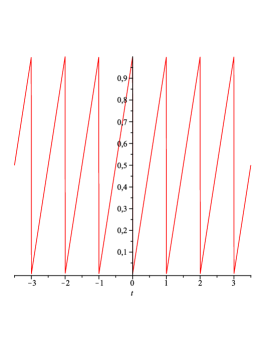
Figure 2. The fractional part $\{t\}$

Let us give the simplest example of the meromorphic functions $S^{L}_{\Lambda}({\mathfrak{p}})(\xi)$ so obtained when $V={\mathbb{R}}$ is one-dimensional. The formulae are written in terms of the fractional part $\{t\}\in[0,1[$ of a real number $t$, such that $t-\{t\}\in{\mathbb{Z}}$ (see Figure 2).

Example 2.6.

Let $V={\mathbb{R}}$, $\Lambda={\mathbb{Z}}$, and consider the cones ${\mathbb{R}}_{\geq 0}$ and ${\mathbb{R}}_{\leq 0}$. Then

$$S_{\mathbb{Z}}^{{{\mathbb{R}}}}(s+{\mathbb{R}}_{\geq 0})(\xi) =-\frac{{\mathrm{e}}^{s\xi}}{\xi}, S_{\mathbb{Z}}^{{{\mathbb{R}}}}(s+{\mathbb{R}}_{\leq 0})(\xi) =\frac{{\mathrm{e}}^{s\xi}}{\xi}$$

while

$$S_{\mathbb{Z}}^{\{0\}}(s+{\mathbb{R}}_{\geq 0})(\xi) ={\mathrm{e}}^{s\xi}\frac{{\mathrm{e}}^{\{-s\}\xi}}{1-{\mathrm{e}}^{\xi}}, S_{\mathbb{Z}}^{\{0\}}(s+{\mathbb{R}}_{\leq 0})(\xi) ={\mathrm{e}}^{s\xi}\frac{{\mathrm{e}}^{-\{s\}\xi}}{1-{\mathrm{e}}^{-\xi}}.$$

For $L\neq\{0\}$, the fact that $S^{L}_{\Lambda}({\mathfrak{p}})$ is actually an element of ${\mathcal{M}}_{\ell}(V^{*})$, is proven in [4], as a consequence of explicit computations which we recall in the next section.

The valuation ${\mathfrak{p}}\mapsto S^{L}_{\Lambda}({\mathfrak{p}})(\xi)$ extends by linearity to the space of linear combinations of indicator functions of semi-rational polyhedra. In particular, if ${\mathfrak{p}}$ is a semi-open polytope defined by rational equations and inequalities, $S^{L}_{\Lambda}({\mathfrak{p}})(\xi)$ is holomorphic and still given by Equation (2.1).

Let us note an obvious but important property.

Lemma 2.7.

If $v\in\Lambda+L$, let $v+{\mathfrak{p}}$ be the shifted polyhedron, then

$$S^{L}_{\Lambda}(v+{\mathfrak{p}})(\xi)={\mathrm{e}}^{\langle\xi,v\rangle}S^{L}_{\Lambda}({\mathfrak{p}})(\xi).$$

2.3. Case of a simplicial cone

We recall some results of [4].

We look first at the discrete generating function. Let ${\mathfrak{c}}$ be a simplicial cone and let $v_{i}$, $i=1,\dots,d$, be lattice generators of its edges (we do not assume that the $v_{i}$’s are primitive). Let ${\mathfrak{b}}=\sum_{i=1}^{d}[0,1\mathclose{[}\,v_{i}$, the corresponding semi-open cell. Let $\operatorname{vol}_{\Lambda}({\mathfrak{b}})=\mathopen{|}\det_{\Lambda}(v_{1},\dots,v_{d})\mathclose{|}$ be its volume with respect to the Lebesgue measure defined by the lattice. Then

$$I_{\Lambda}(s+{\mathfrak{c}})(\xi)={\mathrm{e}}^{{\langle}\xi,s{\rangle}}\frac{(-1)^{d}\operatorname{vol}_{\Lambda}({\mathfrak{b}})}{\prod_{i=1}^{d}{\langle}\xi,v_{i}{\rangle}}.$$ (2.2)

The discrete generating function for the cone can be expressed in terms of that of the semi-open cell:

$$S_{\Lambda}(s+{\mathfrak{c}})(\xi)=S_{\Lambda}(s+{\mathfrak{b}})(\xi)\frac{1}{\prod_{i=1}^{d}(1-{\mathrm{e}}^{{\langle}\xi,v_{i}{\rangle}})}.$$ (2.3)

It follows from (2.3) that the intermediate functions $S_{\Lambda}(s+{\mathfrak{c}})(\xi)$ belong to the space ${\mathcal{M}}_{\ell}(V^{*})$. More precisely, their poles are given by the edges of the cone.

Lemma 2.8.

Let ${\mathfrak{c}}$ be a polyhedral cone with edge generators $v_{i},i=1,\dots,N$ and let $s\in V$. The function $\prod_{i=1}^{N}{\langle}\xi,v_{i}{\rangle}S_{\Lambda}(s+{\mathfrak{c}})(\xi)$ is holomorphic near $\xi=0$.

Proof.

The case where the cone ${\mathfrak{c}}$ is simplicial follows immediately from (2.3), as $S_{\Lambda}(s+{\mathfrak{b}})(\xi)$ is holomorphic. The general case follows from the valuation property, by using a decomposition of ${\mathfrak{c}}$ into simplicial cones without added edges. ∎

Next, we consider the intermediate generating function in the case where ${\mathfrak{c}}$ is simplicial and $L$ is one of its faces. In this case, the intermediate generating function $S^{L}_{\Lambda}(s+{\mathfrak{c}})$ decomposes as a product. For $I\subseteq\{1,\ldots,d\}$, we denote by $L_{I}$ the linear span of the vectors $v_{i}$, $i\in I$. Let $I^{c}$ be the complement of $I$ in $\{1,\ldots,d\}$. For $x\in V$, we write $x=x_{I}+x_{I^{c}}$ with respect to the decomposition $V=L_{I}\oplus L_{I^{c}}$. Thus we identify the quotient $V/L_{I}$ with $L_{I^{c}}$ and we denote the projected lattice by $\Lambda_{I^{c}}\subset L_{I^{c}}$. Write ${\mathfrak{c}}_{I}$ for the cone generated by the vectors $v_{j}$, for $j\in I$ and ${\mathfrak{c}}_{I^{c}}$ for the cone generated by the vectors $v_{j}$, for $j\in I^{c}.$ The projection of the cone ${\mathfrak{c}}$ on $V/L_{I}=L_{I^{c}}$ identifies with ${\mathfrak{c}}_{I^{c}}$. We write also $\xi=\xi_{I}+\xi_{I^{c}}$, with respect to the decomposition $V^{*}=L_{I}^{*}\oplus L_{I^{c}}^{*}$. Then we have the product formula

$$S^{L_{I}}_{\Lambda}(s+{\mathfrak{c}})(\xi)=S_{\Lambda_{I^{c}}}(s_{I^{c}}+{\mathfrak{c}}_{I^{c}})(\xi_{I^{c}})\,I_{\Lambda\cap L_{I}}(s_{I}+{\mathfrak{c}}_{I})(\xi_{I}).$$ (2.4)

Finally, the general case is reduced to the case where ${\mathfrak{c}}$ is simplicial and $L$ is parallel to one of its faces by the Brion–Vergne decomposition (Theorem 19 in [4]), which we summarize in the following proposition and illustrate on an example in Figure 1.

	$\equiv$ $-$
	$\equiv-$   $+$

Figure 1. Two Brion–Vergne decompositions of a cone ${\mathfrak{c}}$ into cones with a face parallel to the subspace $L$, modulo cones with lines.

Proposition 2.9 (Brion–Vergne decomposition).

Let ${\mathfrak{c}}$ be a full-dimensional cone. Then there exists a decomposition of its indicator function $[{\mathfrak{c}}]\equiv\sum_{i}\epsilon_{i}[{\mathfrak{c}}_{i}]$, where each ${\mathfrak{c}}_{i}$ is a simplicial full-dimensional cone with a face parallel to $L$, and the congruence holds modulo the space spanned by indicators functions of cones which contain lines.

Proof.

The case where ${\mathfrak{c}}$ is simplicial is Theorem 19 in [4]. Moreover, for any full-dimensional cone ${\mathfrak{c}}$, there exists a decomposition $[{\mathfrak{c}}]\equiv\sum_{a}\epsilon_{a}[{\mathfrak{c}}_{a}]$ (modulo indicator functions of cones with lines), where ${\mathfrak{c}}_{a}$ are full-dimensional simplicial cones. ∎

Lemma 2.8 holds also for intermediate generating functions $S^{L}_{\Lambda}(s+{\mathfrak{c}})(\xi)$. We will deduce it below from the Poisson summation formula for $S^{L}_{\Lambda}(s+{\mathfrak{c}})(\xi)$, (Theorem 3.1), and the following weaker result.

Lemma 2.10.

For a given cone ${\mathfrak{c}}$, there exist a finite number of vectors $w_{j}\in\Lambda$ such that $\prod_{j=1}^{N}\langle\xi,w_{j}\rangle S^{L}_{\Lambda}(s+{\mathfrak{c}})(\xi)$ is holomorphic near $\xi=0$. In other words, the function $S^{L}_{\Lambda}(s+{\mathfrak{c}})(\xi)$ belongs to the space ${\mathcal{M}}_{\ell}(V^{*})$.

Proof.

By Proposition 2.9 and the valuation property, we have

$$S^{L}_{\Lambda}(s+{\mathfrak{c}})(\xi)=\sum_{i}\epsilon_{i}S^{L}_{\Lambda}(s+{\mathfrak{c}}_{i})(\xi),$$

where each ${\mathfrak{c}}_{i}$ is simplicial with a face parallel to $L$. However, this process may introduce new edges. Finally, when ${\mathfrak{c}}$ is a simplicial cone with a face parallel to $L$, the result follows from Formulas (2.4) and (2.3). ∎

Let us give some examples when $V$ is two-dimensional.

Example 2.11 (positive quadrant).

Let $V={\mathbb{R}}^{2}$, $\Lambda={\mathbb{Z}}^{2}$, and let ${\mathfrak{c}}$ be the positive quadrant. For $s=(s_{1},s_{2})$ and $\xi=(\xi_{1},\xi_{2})$, $S^{L}_{\mathbb{Z}}(s+{\mathfrak{c}})(\xi)$ is given by

$${{\mathrm{e}}^{s_{1}\xi_{1}+s_{2}\xi_{2}}}{\frac{{{\mathrm{e}}^{\{-s_{1}\}\xi_{1}}}{{\mathrm{e}}^{\{-s_{2}\}\xi_{2}}}}{\left(1-{{\mathrm{e}}^{\xi_{1}}}\right)\left(1-{{\mathrm{e}}^{\xi_{2}}}\right)}}, \mbox{ if }L=\{0\},$$ (2.5)

$${{\mathrm{e}}^{s_{1}\xi_{1}+s_{2}\xi_{2}}}\left(\frac{{\mathrm{e}}^{\{-(s_{1}+s_{2})\}\xi_{1}}}{1-{\mathrm{e}}^{\xi_{1}}}-\frac{{\mathrm{e}}^{\{-(s_{1}+s_{2})\}\xi_{2}}}{1-{\mathrm{e}}^{\xi_{2}}}\right)\frac{1}{\xi_{1}-\xi_{2}}, \mbox{ if }L={\mathbb{R}}(1,-1),$$

$${{\mathrm{e}}^{s_{1}\xi_{1}+s_{2}\xi_{2}}}\left(\frac{{\mathrm{e}}^{\{s_{2}-s_{1}\}\xi_{1}}}{1-{\mathrm{e}}^{\xi_{1}}}-\frac{{\mathrm{e}}^{-\{s_{2}-s_{1}\}\xi_{2}}}{1-{\mathrm{e}}^{-\xi_{2}}}\right)\frac{-1}{\xi_{1}+\xi_{2}}, \mbox{ if }L={\mathbb{R}}(1,1).$$

The first formula just follows from (2.3). The second and the third formula follow from Brion–Vergne decompositions and the product formula (2.4). The decomposition used for the third formula, for $L={\mathbb{R}}(1,1)$, is

$$[{\mathfrak{c}}]=[{\mathfrak{c}}_{1}]-[{\mathfrak{c}}_{2}]-[\{x_{1}\geq 0\}],$$

where ${\mathfrak{c}}_{1}=\{x_{2}\geq 0,x_{1}-x_{2}\geq 0\}$ and ${\mathfrak{c}}_{2}=\{x_{1}\geq 0,x_{1}-x_{2}\geq 0\}$, as depicted in Figure 1 (top). The decomposition is not unique. We can compute $S^{L}(s+{\mathfrak{c}})$ using the other Brion–Vergne decomposition, depicted in Figure 1 (bottom),

$$[{\mathfrak{c}}]=-[{\mathfrak{c}}^{\prime}_{1}]+[{\mathfrak{c}}^{\prime}_{2}]+[\{x_{2}\geq 0\}],$$

where ${\mathfrak{c}}^{\prime}_{1}=\{x_{2}\geq 0,x_{1}-x_{2}\leq 0\}$ and ${\mathfrak{c}}^{\prime}_{2}=\{x_{1}\geq 0,x_{1}-x_{2}\leq 0\}$. Then we obtain an expression of $S^{L}(s+{\mathfrak{c}})$ in terms of $\{s_{1}-s_{2}\}$ instead of $\{s_{2}-s_{1}\}$.

2.4. Intermediate sum $S^{L}_{\Lambda}(s+{\mathfrak{c}})(\xi)$ as a function of the pair $(s,\xi)$. Step-polynomials and quasi-polynomials on a rational space.

In this section, ${\mathfrak{c}}$ is a rational cone of full dimension $d$.

2.4.1. The function ${M}^{L}_{\Lambda}(s,{\mathfrak{c}})(\xi)$

We study the properties of $S^{L}_{\Lambda}(s+{\mathfrak{c}})(\xi)$ considered as a function of the two variables $s\in V$, $\xi\in V^{*}$. Actually, as we will see, these properties are more striking and useful when read on the function

$${M}^{L}_{\Lambda}(s,{\mathfrak{c}})(\xi)={\mathrm{e}}^{-\langle\xi,s\rangle}S^{L}_{\Lambda}(s+{\mathfrak{c}})(\xi).$$ (2.6)

The following lemma is immediate.

Lemma 2.12.

Let ${\mathfrak{p}}$ be a semi-rational polyhedron. Let $s\in V$, and let ${M}^{L}_{\Lambda}(s,{\mathfrak{p}})(\xi)={\mathrm{e}}^{-\langle\xi,s\rangle}S^{L}_{\Lambda}(s+{\mathfrak{p}})(\xi)$. Then, for $v\in\Lambda+L$, we have ${M}^{L}_{\Lambda}(s+v,{\mathfrak{p}})(\xi)={M}^{L}_{\Lambda}(s,{\mathfrak{p}})(\xi)$.

Thus the function $s\mapsto{M}^{L}_{\Lambda}(s,{\mathfrak{p}})(\xi)$ can be considered as a function on $V/L$ which is periodic with respect to the projected lattice $\Lambda_{V/L}$. We will often drop the subscript $\Lambda$.

Example 2.13 (Continuation of Example 2.11).

${M}^{L}_{\mathbb{Z}}(s,{\mathfrak{c}})(\xi)$ is given by:

$${\frac{{{\mathrm{e}}^{\{-s_{1}\}\xi_{1}}}{{\mathrm{e}}^{\{-s_{2}\}\xi_{2}}}}{\left(1-{{\mathrm{e}}^{\xi_{1}}}\right)\left(1-{{\mathrm{e}}^{\xi_{2}}}\right)}}, \mbox{ if }L=\{0\},$$ (2.7a)

$$\left(\frac{{\mathrm{e}}^{\{-(s_{1}+s_{2})\}\xi_{1}}}{1-{\mathrm{e}}^{\xi_{1}}}-\frac{{\mathrm{e}}^{\{-(s_{1}+s_{2})\}\xi_{2}}}{1-{\mathrm{e}}^{\xi_{2}}}\right)\frac{1}{\xi_{1}-\xi_{2}}, \mbox{ if }L={\mathbb{R}}(1,-1),$$ (2.7b)

$$\left(\frac{{\mathrm{e}}^{\{s_{2}-s_{1}\}\xi_{1}}}{1-{\mathrm{e}}^{\xi_{1}}}-\frac{{\mathrm{e}}^{-\{s_{2}-s_{1}\}\xi_{2}}}{1-{\mathrm{e}}^{-\xi_{2}}}\right)\frac{-1}{\xi_{1}+\xi_{2}}, \mbox{ if }L={\mathbb{R}}(1,1).$$ (2.7c)

2.4.2. Step-polynomials and quasi-polynomials on $V$

A crucial role in our study is played by the individual homogeneous components $S^{L}(s+{\mathfrak{c}})_{[m]}(\xi)$ and ${M}^{L}(s,{\mathfrak{c}})_{[m]}(\xi)$. A pleasant feature is that, when ${\mathfrak{c}}$ is fixed, the homogeneous component of $\xi$-degree $m$ can be viewed as a function of $s\in V$ with values in a finite-dimensional vector space, namely the space of rational functions of homogeneous $\xi$-degree $m$ which can be written in the form $\frac{P(\xi)}{\prod_{j}\langle\xi,w_{j}\rangle}$, where the family of vectors $w_{j}$ is given by Lemma 2.10.

We introduce an algebra of functions on $V\times V^{*}$ in order to describe these homogeneous components. Let us start with an example.

Example 2.14 (Continuation of Example 2.11).

Let $L={\mathbb{R}}(1,1)$. We expand (2.7c), using the Bernoulli polynomials, defined by

$${\mathrm{e}}^{tz}\frac{z}{{\mathrm{e}}^{z}-1}=\sum_{n=0}^{\infty}\frac{B_{n}(t)}{n!}z^{n},$$ (2.8)

obtaining

$${M}^{L}(s,{\mathfrak{c}})_{[-2]}(\xi) =\frac{1}{\xi_{1}\xi_{2}},$$

$${M}^{L}(s,{\mathfrak{c}})_{[-1]}(\xi) =0,$$

$${M}^{L}(s,{\mathfrak{c}})_{[0]}(\xi) =\frac{B_{2}(\{s_{2}-s_{1}\})}{2}=\frac{\{s_{2}-s_{1}\}^{2}-\{s_{2}-s_{1}\}+\frac{1}{6}}{2},$$

$${M}^{L}(s,{\mathfrak{c}})_{[1]}(\xi) =\frac{B_{3}(\{s_{2}-s_{1}\})}{3!}(\xi_{1}-\xi_{2})$$

$$=\frac{\{s_{2}-s_{1}\}^{3}-\frac{3}{2}\{s_{2}-s_{1}\}^{2}+\frac{1}{2}\{s_{2}-s_{1}\}}{6}(\xi_{1}-\xi_{2}).$$

From these formulas, we obtain

$$S^{L}(s+{\mathfrak{c}})_{[-2]}(\xi) =\frac{1}{\xi_{1}\xi_{2}},$$

$$S^{L}(s+{\mathfrak{c}})_{[-1]}(\xi) =\frac{s_{1}\xi_{1}+s_{2}\xi_{2}}{\xi_{1}\xi_{2}},$$

$$S^{L}(s+{\mathfrak{c}})_{[0]}(\xi) =\frac{(s_{1}\xi_{1}+s_{2}\xi_{2})^{2}+\xi_{1}\xi_{2}(\{s_{2}-s_{1}\}^{2}-\{s_{2}-s_{1}\}+\frac{1}{6})}{2\xi_{1}\xi_{2}}.$$

We observe that the numerators above are written as polynomial functions of $s_{1},s_{2},\{s_{2}-s_{1}\},\xi_{1},\xi_{2}$. We next describe the general case.

Let $V^{*}_{\mathbb{Q}}=\Lambda^{*}\otimes{\mathbb{Q}}$ be the set of rational elements of $V^{*}$.

Definition 2.15.

${\mathcal{Q}}(V)$ is the algebra of functions on $V$ generated by the functions $s\mapsto\{\langle\lambda,s\rangle\}$, where $\lambda\in V^{*}_{\mathbb{Q}}$. An element of ${\mathcal{Q}}(V)$ is called a (rational) step-polynomial on $V$.

Remark 2.16.

Note that there are many relations between these generators. For example, if $V={\mathbb{R}}$, consider for $\lambda\in{\mathbb{Q}}$ the function $f_{\lambda}(s)=1-(\{\lambda s\}+\{-\lambda s\})$, which is $1$ if $\lambda s$ is an integer and $0$ otherwise. Then we have the polynomial relation $f_{1}(s)=f_{2}(s)f_{3}(s)$.

Since the generators $s\mapsto\{\langle\lambda,s\rangle\}$ are bounded functions, it follows that a step-polynomial is a bounded function on $V$.

The space ${\mathcal{Q}}(V)$ has a natural filtration, where ${\mathcal{Q}}_{[\leq k]}(V)$ is the subspace generated by products of at most $k$ functions $\{\langle\lambda,s\rangle\}$.

For $\eta\in\Lambda^{*}$, the function $s\mapsto\{\langle\eta,s\rangle\}$ is $\Lambda$-periodic. For a given step-polynomial $f(s)$, let $q\in{\mathbb{N}}$ be such that $q\lambda\in\Lambda^{*}$ for all the $\lambda$’s involved in an expression of $f(s)$ (such an expression is not unique). Then $f$ is $q\Lambda$-periodic.

Next, we consider the algebra of functions on $V$ generated by ${\mathcal{Q}}(V)$ and ${\mathcal{P}}(V)$, where ${\mathcal{P}}(V)$ is the algebra of polynomial functions on $V$. It is clear that this algebra is the tensor product ${\mathcal{Q}}(V)\otimes{\mathcal{P}}(V)$. We denote it by ${\mathcal{Q}}{\mathcal{P}}(V)$.

Definition 2.17.

The elements of ${\mathcal{Q}}{\mathcal{P}}(V)={\mathcal{Q}}(V)\otimes{\mathcal{P}}(V)$ are called quasi-polynomials on $V$.

Now, let $\Psi$ be a finite subset of $V_{\mathbb{Q}}^{*}$. There corresponds a subalgebra of quasi-polynomials on $V$.

Definition 2.18.

1. ${\mathcal{Q}}^{\Psi}(V)$ is the algebra of functions on $V$ generated by the functions $s\mapsto\{\langle\eta,s\rangle\}$, with $\eta\in\Psi$.

2. ${\mathcal{Q}}^{\Psi}_{[\leq k]}(V)$ is the subspace of ${\mathcal{Q}}^{\Psi}(V)$ generated by products of at most $k$ functions $\{\langle\eta,s\rangle\}$, with $\eta\in\Psi$.

3. ${\mathcal{Q}}{\mathcal{P}}^{\Psi}(V)$ is the algebra of functions on $V$ generated by ${\mathcal{Q}}^{\Psi}(V)$ and ${\mathcal{P}}(V)$.

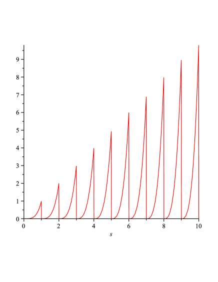
Figure 3. The function $s\mapsto\{s\}^{3}s$

The quasi-polynomials in ${\mathcal{Q}}{\mathcal{P}}^{\Psi}(V)$ are piecewise polynomial, in a sense which we describe now.

Definition 2.19.

Let $\Psi$ be a finite subset of $V_{\mathbb{Q}}^{*}$. We consider the hyperplanes in $V$ defined by the equations

$$\langle\eta,x\rangle=n\quad\mbox{ for }\eta\in\Psi\mbox{ and }n\in{\mathbb{Z}}.$$

A connected component of the complement of the union of these hyperplanes in $V$ is called a $\Psi$-alcove.

Thus, an alcove is the interior of a polyhedron whose faces are some of the hyperplanes above. If $\Psi$ generates $V^{*}$, all alcoves are bounded. Otherwise, they are unbounded. If $s$ is any element of $V$, and $v\in V$ is a fixed element such that $\langle\eta,v\rangle\neq 0$ for $\eta\in\Psi$, then the curve $s+tv$ is contained in a $\Psi$-alcove for small $t<0$.

If $\eta\in\Psi$, the restriction to any $\Psi$-alcove of the function $s\mapsto\{\langle\eta,s\rangle\}$ is affine. Therefore the restriction of a quasi-polynomial $f(s)\in{\mathcal{Q}}_{[\leq k]}^{\Psi}(V)\otimes{\mathcal{P}}_{[r]}(V)$ to an alcove is a polynomial in $s$ of degree $\leq k+r$. This motivates the following definition.

Definition 2.20.

1. A function $f(s)\in{\mathcal{Q}}_{[\leq k]}^{\Psi}(V)\otimes{\mathcal{P}}_{[r]}(V)$ is said to be of polynomial degree $r$ and of local degree (at most) $k+r$.

2. We define ${\mathcal{Q}}{\mathcal{P}}^{\Psi}_{[\leq q]}(V)$ to be the subspace of quasi-polynomials of local degree at most $q$.

In Figure 3, we draw the graph of a quasi-polynomial function on ${\mathbb{R}}$ (with $\Lambda={\mathbb{Z}}$ and $\Psi=\{1\}$) of local degree $4$.

2.4.3. Properties of homogeneous components of generating functions of shifted cones

We start with the case $L=\{0\}$. Given a cone ${\mathfrak{c}}\subset V$, we define a subalgebra of step-polynomials associated with ${\mathfrak{c}}$. The fundamental fact here is the existence of a decomposition of the indicator function of ${\mathfrak{c}}$ as a signed sum

$$[{\mathfrak{c}}]\equiv\sum_{{\mathfrak{u}}}\epsilon_{{\mathfrak{u}}}[{\mathfrak{u}}],$$ (2.9)

where the cones ${\mathfrak{u}}$ are unimodular, and the congruence is modulo the space spanned by indicator functions of cones which contain lines. If ${\mathfrak{c}}$ is full-dimensional, we can assume that the cones ${\mathfrak{u}}$ are also full-dimensional, see [8] for instance. By the valuation property, we have

$$S(s+{\mathfrak{c}})(\xi)=\sum_{{\mathfrak{u}}}\epsilon_{{\mathfrak{u}}}S(s+{\mathfrak{u}})(\xi).$$

For each unimodular cone ${\mathfrak{u}}$ in (2.9), let $v_{j}^{\mathfrak{u}}\in\Lambda$, $1\leq j\leq d$, be the primitive generators of the cone ${\mathfrak{u}}$, and let $\eta_{j}^{{\mathfrak{u}}}\in\Lambda^{*}$, $1\leq j\leq d$, be the dual basis.

Definition 2.21.

We denote by $\Psi_{\mathfrak{c}}\subset\Lambda^{*}$ the set of all $\eta_{j}^{{\mathfrak{u}}}$, for $j=1,\ldots,d$, where ${\mathfrak{u}}$ runs over the set of unimodular cones entering in the decomposition (2.9) of $[{\mathfrak{c}}]$.

$\Psi_{\mathfrak{c}}$ depends of the choice of the decomposition, but we do not record it in the notation, for brevity.

We can now state the important bidegree properties of the homogeneous components of the functions $S(s+{\mathfrak{c}})(\xi)$ and ${M}(s,{\mathfrak{c}})(\xi)$. Here “bidegree” refers to the interaction between the (local) degree in $s$ and the homogeneous degree in $\xi$.

Theorem 2.22.

Let $m\in{\mathbb{Z}}$.

1. The function $(s,\xi)\mapsto{M}(s,{\mathfrak{c}})_{[m]}(\xi)$ belongs to the space

   $${\mathcal{Q}}_{[\leq m+d]}^{\Psi_{\mathfrak{c}}}(V)\otimes{\mathcal{R}}_{[m]}(V^{*}).$$

2. The function $(s,\xi)\mapsto S(s+{\mathfrak{c}})_{[m]}(\xi)$ belongs to the space

   $${\mathcal{Q}}{\mathcal{P}}^{\Psi_{\mathfrak{c}}}_{[\leq m+d]}(V)\otimes{\mathcal{R}}_{[m]}(V^{*}).$$

   More precisely,

   $$S(s+{\mathfrak{c}})_{[m]}(\xi)=\sum_{r=0}^{m+d}\frac{\langle\xi,s\rangle^{r}}{r!}{M}(s,{\mathfrak{c}})_{[m-r]}(\xi).$$

3. The homogeneous component in $\xi$ of lowest degree has degree $m=-d$ and does not depend on $s$. It is given by the integral

   $$S(s+{\mathfrak{c}})_{[-d]}(\xi)={M}(s,{\mathfrak{c}})_{[-d]}(\xi)=I({\mathfrak{c}})(\xi).$$

To rephrase (ii), we can say that the numerator of the homogeneous component $S(s+{\mathfrak{c}})_{[m]}(\xi)$ is a quasi-polynomial function of $s$ (with coefficients polynomials in $\xi$), and the local degree in $s$ of this quasi-polynomial (and so its complexity) grows with the homogeneity degree $m$ in $\xi$.

Proof.

Let ${\mathfrak{u}}$ be one of the unimodular cones in the decomposition of $[{\mathfrak{c}}]$. We write $\xi=\sum_{j}\xi_{j}\eta_{j}^{\mathfrak{u}}$. Then $S(s+{\mathfrak{u}})(\xi)$ is directly computed by summing a multiple geometric series (cf. Example 2.6), hence

$${M}(s,{\mathfrak{u}})(\xi) =\exp\Bigl{(}{\sum_{j}\{-\langle\eta_{j}^{u},s\rangle\}\xi_{j}}\Bigr{)}\prod_{j=1}^{d}\frac{1}{1-{\mathrm{e}}^{\xi_{j}}},$$

$${M}(s,{\mathfrak{u}})_{[m]}(\xi) =\sum_{k=0}^{d+m}\frac{(\sum_{j}\{-\langle\eta_{j}^{u},s\rangle\}\xi_{j})^{k}}{k!}\biggl{(}\prod_{j=1}^{d}\frac{1}{1-{\mathrm{e}}^{\xi_{j}}}\biggr{)}_{[m-k]}.$$

In this formula, it is clear that the $k$-th term belongs to ${\mathcal{Q}}_{[\leq k]}^{\Psi_{\mathfrak{c}}}(V)\otimes{\mathcal{R}}_{[m]}(V^{*})$. As $k\leq m+d$, we obtain (i). The homogeneous components $S(s+{\mathfrak{c}})_{[m]}(\xi)$ are immediately computed out of those of ${M}(s,{\mathfrak{c}})(\xi)$, hence (ii). Part (iii) was proved in [2], Lemma 16. ∎

Now let $L\subseteq V$ be any rational subspace. In order to obtain a similar result for the intermediate generating function $S^{L}(s+{\mathfrak{c}})(\xi)$, we follow the steps of the proof of Lemma 2.10. First, we decompose $[{\mathfrak{c}}]$ into a signed sum of simplicial cones with a face parallel to $L$. For each of these cones, we decompose the projected cone in $V/L$ into a signed sum of cones which are unimodular with respect to the projected lattice $\Lambda_{V/L}$. We thus have a collection of unimodular cones ${\mathfrak{u}}\subset V/L$. When $(V/L)^{*}$ is identified with $L^{\perp}\subset V^{*}$, the dual lattice $(\Lambda_{V/L})^{*}$ is identified with $\Lambda^{*}\cap L^{\perp}$. For each ${\mathfrak{u}}$, we let $v_{j}^{\mathfrak{u}}\in\Lambda_{V/L}$ be primitive edge generators of ${\mathfrak{u}}$ and consider the dual basis $\eta_{j}^{\mathfrak{u}}\in\Lambda^{*}\cap L^{\perp}$.

Definition 2.23.

We denote by $\Psi_{\mathfrak{c}}^{L}\subset\Lambda^{*}\cap L^{\perp}$ the set of all $\eta_{j}^{\mathfrak{u}}$.

Then the functions in ${\mathcal{Q}}^{\Psi_{\mathfrak{c}}^{L}}(V)$ are functions on $V/L$ and are $\Lambda_{V/L}$-periodic. Using the product formula (2.4), the proof of the following theorem is similar to the case $L=\{0\}$ (Theorem 2.22).

Theorem 2.24.

Let $m\in{\mathbb{Z}}$.

1. The function $(s,\xi)\mapsto{M}^{L}(s,{\mathfrak{c}})_{[m]}(\xi)$ belongs to the space

   $${\mathcal{Q}}_{[\leq m+d]}^{\Psi_{\mathfrak{c}}^{L}}(V)\otimes{\mathcal{R}}_{[m]}(V^{*}).$$

2. The function $(s,\xi)\mapsto S^{L}(s+{\mathfrak{c}})_{[m]}(\xi)$ belongs to the space

   $${\mathcal{Q}}{\mathcal{P}}_{[\leq m+d]}^{\Psi_{\mathfrak{c}}^{L}}(V)\otimes{\mathcal{R}}_{[m]}(V^{*}).$$

   More precisely

   $$S^{L}(s+{\mathfrak{c}})_{[m]}(\xi)=\sum_{r=0}^{m+d}\frac{\langle\xi,s\rangle^{r}}{r!}{M}^{L}(s,{\mathfrak{c}})_{[m-r]}(\xi).$$ (2.10)

3. The homogeneous component in $\xi$ of lowest degree has degree $m=-d$ and does not depend on $s$. It is given by the integral

   $$S^{L}(s+{\mathfrak{c}})_{[-d]}(\xi)={M}^{L}(s,{\mathfrak{c}})_{[-d]}(\xi)=I({\mathfrak{c}})(\xi).$$

Remark 2.25.

If $L=V$, then $\Psi_{\mathfrak{c}}^{L}$ is empty, hence ${\mathcal{Q}}^{\Psi_{\mathfrak{c}}^{L}}(V)$ is just the scalars. Indeed, ${\mathrm{e}}^{-\langle\xi,s\rangle}I(s+{\mathfrak{c}})(\xi)=I({\mathfrak{c}})(\xi)$ does not depend on $s$.

Remark 2.26.

As we showed in [2, Theorems 31 and 38] and [4, Theorems 24 and 28], the computation of these functions and their homogeneous components can be made effective, and the bidegree structure, i.e., the interaction of the local degree in $s$ and the homogeneous degree in $\xi$, takes a key role in extracting the refined asymptotics. We have developed Maple implementation of such algorithms, which work with a symbolic vertex $s$; the resulting formulas are naturally valid for any real vector $s\in V$.

2.5. One-sided continuity

The meromorphic functions $M^{L}(s,{\mathfrak{c}})(\xi)$ and $S^{L}(s+{\mathfrak{c}})(\xi)$ and their homogeneous components $M^{L}(s,{\mathfrak{c}})_{[m]}(\xi)$ and $S^{L}(s+{\mathfrak{c}})_{[m]}(\xi)$ enjoy some continuity properties when $s$ tends to $s_{0}$ along some directions that we will describe. Let us look again at the simplest example (Example 2.6). We have

$$S_{\mathbb{Z}}^{\{0\}}(s+{\mathbb{R}}_{\geq 0})(\xi)={\mathrm{e}}^{s\xi}\frac{{\mathrm{e}}^{\{-s\}\xi}}{1-{\mathrm{e}}^{\xi}},$$

and

$$S_{\mathbb{Z}}^{\{0\}}(s+{\mathbb{R}}_{\leq 0})(\xi)={\mathrm{e}}^{s\xi}\frac{{\mathrm{e}}^{-\{s\}\xi}}{1-{\mathrm{e}}^{-\xi}}.$$

Then observe that as functions of $s$, the first formula is continuous from the left, while the second formula is continuous from the right. These directions are the opposite of the direction of the corresponding cones, and the result is intuitively clear. For instance, the set $(s+{\mathbb{R}}_{\geq 0})\cap{\mathbb{Z}}$ itself does not change when $s$ is moved slightly to the left; but it does change if $s$ is moved slightly to the right from an integer.

We state a generalization of this result in higher dimensions. In order to state the result, we observe that, in Theorem 2.24, the infinite-dimensional space ${\mathcal{R}}_{[m]}(V^{*})$ can be replaced by the following finite-dimensional subspace.

Definition 2.27.

Let $(v_{j})_{j=1}^{N}$ be a set of vectors in $V$ such that the function $\prod_{j=1}^{N}\langle\xi,v_{j}\rangle S^{L}(s+{\mathfrak{c}})(\xi)$ is holomorphic near $\xi=0$. Then as rational functions of $\xi$, both ${M}^{L}(s,{\mathfrak{c}})_{[m]}(\xi)$ and $S^{L}(s+{\mathfrak{c}})_{[m]}(\xi)$ lie in the finite-dimensional space of functions $f(\xi)$ such that $\prod_{j=1}^{N}\langle\xi,v_{j}\rangle f(\xi)$ is a polynomial of degree $m+N$. We denote this space by $\frac{1}{\prod_{j=1}^{N}v_{j}}{\mathcal{P}}_{[m+N]}(V^{*})$.

Figure 4. One-sided continuity of the functions $M^{L}(s,{\mathfrak{c}})(\xi)$ and $S^{L}(s+{\mathfrak{c}})(\xi)$ and their homogeneous components, as functions of the apex $s$. Discontinuities arise when one of the copies of $L$ in $L+\Lambda$ intersects the boundary of the cone $s+{\mathfrak{c}}$; in this case we still have one-sided continuity when we move in a direction $v\in L-{\mathfrak{c}}$.

Figure 5. One-sided continuity of the functions $M^{L}(s,{\mathfrak{c}})(\xi)$ and $S^{L}(s+{\mathfrak{c}})(\xi)$ and their homogeneous components, as functions of the apex $s$. In this example, $L-{\mathfrak{c}}=V$, and thus the functions actually depend continuously on $s$.

Proposition 2.28.

Let $(v_{j})_{j=1}^{N}$ be a set of vectors in $V$ such that the function $\prod_{j=1}^{N}\langle\xi,v_{j}\rangle S^{L}(s+{\mathfrak{c}})(\xi)$ is holomorphic near $\xi=0$.

1. The restriction of $s\mapsto{M}^{L}(s,{\mathfrak{c}})_{[m]}(\xi)$ and $s\mapsto S^{L}(s+{\mathfrak{c}})_{[m]}(\xi)$ to a $\Psi_{\mathfrak{c}}^{L}$-alcove ${\mathfrak{a}}\subset V$ are polynomial functions of $s$ with values in the finite-dimensional space $\frac{1}{\prod_{j=1}^{N}v_{j}}{\mathcal{P}}_{[m+N]}(V^{*})$.

2. Let $s\in V$. For any $v\in L-{\mathfrak{c}}$, we have the following one-sided limit (cf. Figures 4 and 5),

   $$\lim_{\begin{subarray}{c}t\to 0\\ t>0\end{subarray}}{M}^{L}(s+tv,{\mathfrak{c}})_{[m]}(\xi)={M}^{L}(s,{\mathfrak{c}})_{[m]}(\xi).$$

Proof.

Part (i) is an immediate consequence of Theorem 2.24.

For part (ii) we assume that ${\mathfrak{c}}$ is pointed, otherwise there is nothing to prove. Recall the definition of $S^{L}(s+{\mathfrak{c}})(\xi)$. Fix $s_{0}\in V$. There is a non-empty open subset $U\subset V^{*}_{\mathbb{C}}$ such that for $s$ near $s_{0}$ and $\xi\in U$, the following sum

$$S^{L}(s+{\mathfrak{c}})(\xi)=\sum_{y\in\Lambda_{V/L}}\int_{(s+{\mathfrak{c}})\cap(y+L)}{\mathrm{e}}^{{\langle}\xi,x{\rangle}}\,\mathrm{d}x$$

converges uniformly to a holomorphic function of $\xi$. Intuitively, the lemma is based on the observation that if $v\in L-{\mathfrak{c}}$ and $t>0$ is small enough, then the projections of the shifted cones $s+{\mathfrak{c}}$ and $s+tv+{\mathfrak{c}}$ on $V/L$ have the same lattice points.

Let us look first at the extreme cases, $L=\{0\}$ or $L=V$. If $L=\{0\}$, for $v\in L-{\mathfrak{c}}$ and $t>0$ small enough, the shifted cones $s+{\mathfrak{c}}$ and $s+tv+{\mathfrak{c}}$ have the same lattice points, hence $S(s+tv+{\mathfrak{c}})(\xi)=S(s+{\mathfrak{c}})(\xi)$ for $\xi\in U$. It follows that these meromorphic functions are equal. If $L=V$, then $S^{L}(s+{\mathfrak{c}})(\xi)=I(s+{\mathfrak{c}})(\xi)={\mathrm{e}}^{\langle\xi,s\rangle}I({\mathfrak{c}})(\xi)$ depends continuously on the apex $s$.

Now, let $L$ be arbitrary. Let $v\in L-{\mathfrak{c}}$ and $t>0$ small enough. Then the projections of the shifted cones $s+{\mathfrak{c}}$ and $s+tv+{\mathfrak{c}}$ on $V/L$ have the same lattice points. Consider a given $y\in\Lambda_{V/L}$. If $y$ does not lie in this projection, then $\int_{(s+tv+{\mathfrak{c}})\cap(y+L)}{\mathrm{e}}^{{\langle}\xi,x{\rangle}}\,\mathrm{d}x=0$. Otherwise, it is clear that the integral $\int_{(s+tv+{\mathfrak{c}})\cap(y+L)}{\mathrm{e}}^{{\langle}\xi,x{\rangle}}\,\mathrm{d}x$ depends continuously on $t$. Hence, for all $y\in\Lambda_{V/L}$, we have

$$\lim_{\begin{subarray}{c}t\to 0\\ t>0\end{subarray}}\;\int_{(s+tv+{\mathfrak{c}})\cap(y+L)}{\mathrm{e}}^{{\langle}\xi,x{\rangle}}\,\mathrm{d}x=\int_{(s+{\mathfrak{c}})\cap(y+L)}{\mathrm{e}}^{{\langle}\xi,x{\rangle}}\,\mathrm{d}x,$$

uniformly for $\xi\in U$. Therefore

$$\lim_{\begin{subarray}{c}t\to 0\\ t>0\end{subarray}}S^{L}(s+tv+{\mathfrak{c}})(\xi)=S^{L}(s+{\mathfrak{c}})(\xi),$$

uniformly for $\xi\in U$. The difficulty is that $0\notin U$. To deal with it, it is enough to prove that there exists a finite set of vectors $v_{j}\in V$ and a ball $B\subset V^{*}_{\mathbb{C}}$ of center $0$ intersecting $U$, such that $\prod_{j=1}^{N}\langle\xi,v_{j}\rangle S^{L}(s+{\mathfrak{c}})(\xi)$ is holomorphic and uniformly bounded on $B$, for $s$ in neighborhood of a given $s_{0}$. By the Montel compactness theorem, it will follow that

$$\lim_{\begin{subarray}{c}t\to 0\\ t>0\end{subarray}}\;\prod_{j=1}^{N}\langle\xi,v_{j}\rangle S^{L}(s+tv+{\mathfrak{c}})(\xi)=\prod_{j=1}^{N}\langle\xi,v_{j}\rangle S^{L}(s+{\mathfrak{c}})(\xi)$$

uniformly for $\xi\in B$, therefore the limit will hold also for homogeneous components.

To prove the uniform boundedness property above, we use the Brion–Vergne decomposition (Proposition 2.9) of ${\mathfrak{c}}$ as a signed sum of simplicial cones, each with a face parallel to $L$, modulo cones with lines. We take $(v_{j})$ to be the collection of all edge generators for all these cones. So now we need only prove uniform boundedness for a simplicial cone for which $L$ is a face. By the product formula, we are reduced to the extreme cases $S(s+{\mathfrak{c}})$ and $I(s+{\mathfrak{c}})$. The latter is continuous with respect to $s$, so uniform boundedness holds. For the discrete sum, uniform boundedness follows from Formula (2.3). ∎

Remark 2.29.

Although the result is intuitively clear, a proof is needed because we have an infinite sum. Indeed, consider the sequence of holomophic functions $f_{n}(z)=\frac{{\mathrm{e}}^{nz}-1}{nz}$. This sequence converges pointwise to $0$ for $\Re z<0$. However, the homogeneous components $\frac{n^{k}}{(k+1)!}z^{k}$ do not converge to $0$.

Example 2.30.

Let us look again at the positive quadrant from Examples 2.11 and 2.14, with $L={\mathbb{R}}(1,1)$ (see Figure 5). By means of the Brion–Vergne decomposition of the quadrant depicted in Figure 1 (top), we computed a formula for ${M}^{L}(s,{\mathfrak{c}})_{[m]}(\xi)$ in terms of the Bernoulli polynomial $B_{m+2}(\{s_{2}-s_{1}\})$. Let $v_{1}<0,v_{2}<0$, so $v\in-{\mathfrak{c}}$. Then $\lim_{t\to 0,t>0}\{s_{2}+tv_{2}-s_{1}-tv_{1}\}=\{s_{2}-s_{1}\}$ if $v_{2}-v_{1}>0$. But if $v_{2}-v_{1}<0$ and $s_{2}-s_{1}\in{\mathbb{Z}}$, then $\lim_{t\to 0,t>0}\{s_{2}+tv_{2}-s_{1}-tv_{1}\}=1$ while $\{s_{2}-s_{1}\}=0$. However, observe that if $t>0$ is small, then $s_{2}+tv_{2}-s_{1}-tv_{1}\notin{\mathbb{Z}}$, hence

$$\{s_{2}+tv_{2}-s_{1}-tv_{1}\}=1-\{-(s_{2}+tv_{2}-s_{1}-tv_{1})\}.$$

Thus the limit statement in the lemma holds also for $v_{2}-v_{1}<0$, due to the property of Bernoulli polynomials: $B_{n}(1-u)=(-1)^{n}B_{n}(u)$.

Another way to reach this conclusion is to use the other Brion–Vergne decomposition of the quadrant, depicted in Figure 1 (bottom). Then we obtain an expression of $S^{L}(s+{\mathfrak{c}})$ in terms of $\{s_{1}-s_{2}\}$ instead of $\{s_{2}-s_{1}\}$. We see here the well-known link between the valuation property of generating functions and the functional equation of Bernoulli polynomials.

Remark 2.31.

Figure 6. One-sided continuity of the functions $M^{L}(s,{\mathfrak{c}})(\xi)$ and $S^{L}(s+{\mathfrak{c}})(\xi)$ and their homogeneous components, as functions of the apex $s$. In this example, $L-{\mathfrak{c}}$ is a halfspace, and so Proposition 2.28 only predicts one-sided continuity. However, the functions actually depend continuously on $s$.

Actually, the functions $s\mapsto{M}^{L}(s,{\mathfrak{c}})_{[m]}(\xi)$ and $s\mapsto S^{L}(s+{\mathfrak{c}})_{[m]}(\xi)$ enjoy stronger continuity properties on the boundary of alcoves than claimed in Proposition 2.28. For instance, for a two-dimensional cone ${\mathfrak{c}}$, if $L$ is not parallel to an edge of the cone and $L\neq\{0\}$, it is intuitively clear that these functions depend continuously on $s$, see Figure 6. It is also enlightening to check the continuity property on the formulas.

3. Poisson summation formula and Fourier series of $s\mapsto{M}^{L}(s,{\mathfrak{c}})(\xi)={\mathrm{e}}^{-\langle\xi,s\rangle}S^{L}(s+{\mathfrak{c}})(\xi)$

The Poisson summation formula reads, for suitable functions $\phi$ on $V$,

$$\sum_{x\in\Lambda}\phi(x)=\sum_{\gamma\in\Lambda^{*}}{\hat{\phi}}(2\pi\gamma).$$

Here $\hat{\phi}$ is the Fourier transform of $\phi$, with respect to the Lebesgue measure defined by $\Lambda$. Let us apply formally this formula to the series

$$S(s+{\mathfrak{c}})(\xi)=\sum_{x\in(s+{\mathfrak{c}})\cap\Lambda}{\mathrm{e}}^{\langle\xi,x\rangle}=\sum_{x\in\Lambda}{\mathrm{e}}^{\langle\xi,x\rangle}{[s+{\mathfrak{c}}]}(x).$$ (3.1)

Formally, the Fourier transform of $\phi(x)={\mathrm{e}}^{\langle\xi,x\rangle}{[s+{\mathfrak{c}}]}(x)$ is

$$\hat{\phi}(2\pi\gamma)=\int_{s+{\mathfrak{c}}}{\mathrm{e}}^{\langle\xi+2i\pi\gamma,x\rangle}\,\mathrm{d}x=I(s+{\mathfrak{c}})(\xi+2i\pi\gamma).$$

So, heuristically, we obtain

$$S(s+{\mathfrak{c}})(\xi)=\sum_{\gamma\in\Lambda^{*}}I(s+{\mathfrak{c}})(\xi+2i\pi\gamma).$$ (3.2)

This heuristic result admits a precise formulation given in Corollary 3.3 below, valid also for intermediate generating functions $S^{L}(s+{\mathfrak{c}})$.

For a given $\gamma\in\Lambda^{*}$, the function $\xi\mapsto I(s+{\mathfrak{c}})(\xi+2i\pi\gamma)$ belongs also to ${\mathcal{M}}_{\ell}(V^{*})$. More precisely, if $(v_{j})$ are the generators of ${\mathfrak{c}}$, this function has simple hyperplane singularities near $\xi=0$, with singular hyperplanes given by $\langle\xi,v_{j}\rangle=0$, for the indices $j$ such that $\langle\gamma,v_{j}\rangle=0$. Thus we can also define the homogeneous components $I(s+{\mathfrak{c}})(\xi+2i\pi\gamma)_{[m]}$, and $I(s+{\mathfrak{c}})(\xi+2i\pi\gamma)_{[m]}$ belongs to ${\mathcal{R}}_{[m]}(V^{*})$. For example, for $n\neq 0$, the expansion of $-\frac{1}{\xi+2i\pi n}$ in homogeneous components is

$$-\frac{1}{\xi+2i\pi n}=\sum_{m=0}^{\infty}\frac{(-1)^{m+1}}{(2i\pi n)^{m+1}}\xi^{m}.$$

3.1. Fourier series of ${M}^{L}(s,{\mathfrak{c}})(\xi)$

The starting point is, once again, the important fact that the function

$$s\mapsto{M}^{L}(s,{\mathfrak{c}})(\xi)={\mathrm{e}}^{-\langle\xi,s\rangle}S^{L}(s+{\mathfrak{c}})(\xi),$$

which is a function on $V/L$, is periodic with respect to the projected lattice $\Lambda_{V/L}$. Each homogeneous component ${M}^{L}(s,{\mathfrak{c}})_{[m]}(\xi)$ is periodic as well, and piecewise polynomial, hence bounded. We are going to compute its Fourier coefficients.

Theorem 3.1.

Let ${\mathfrak{c}}\subset V$ be a full-dimensional cone with edge generators $v_{1},\dots,v_{N}$. Let $L\subseteq V$ be a rational linear subspace. For $s\in V$, let ${M}^{L}(s,{\mathfrak{c}})(\xi)={\mathrm{e}}^{-\langle\xi,s\rangle}S^{L}(s+{\mathfrak{c}},\Lambda)(\xi)$. For every $m\in{\mathbb{Z}}$, consider the homogeneous component ${M}^{L}(s,{\mathfrak{c}})_{[m]}(\xi)$ as a periodic function of $s\in V$ with values in the finite-dimensional space $\frac{1}{\prod_{j=1}^{N}v_{j}}{\mathcal{P}}_{[m+N]}(V^{*})$ of rational functions in $\xi$ of homogeneous degree $m$ whose denominator divides $\prod_{j=1}^{N}\langle\xi,v_{j}\rangle$. Then the Fourier series of ${M}^{L}(s,{\mathfrak{c}})_{[m]}(\xi)$ is

$${M}^{L}(s,{\mathfrak{c}})_{[m]}(\xi)=\sum_{\gamma\in\Lambda^{*}\cap L^{\perp}}{\mathrm{e}}^{\langle 2i\pi\gamma,s\rangle}I({\mathfrak{c}})(\xi+2i\pi\gamma)_{[m]}.$$ (3.3)

Proof.

Given ${\mathfrak{c}}$ and $L$, we decompose $[{\mathfrak{c}}]\equiv\sum_{i}\epsilon_{i}[{\mathfrak{c}}_{i}]$, where now each cone ${\mathfrak{c}}_{i}$ is simplicial with a face parallel to $L$ and full-dimensional (Proposition 2.9). By linearity of homogeneous components and Fourier coefficients, we can assume that ${\mathfrak{c}}$ is simplicial with a face parallel to $L$. Then we write $S^{L}(s+{\mathfrak{c}})(\xi)$ as a tensor product of a discrete generating function in dimension $k=\operatorname{codim}L$ with a continuous one in dimension $\dim L$. Thus, we are reduced to the cases $L=\{0\}$ and $L=V$.

We observe that the result is true when $L=V$, as ${M}^{V}(s,{\mathfrak{c}})(\xi)=I({\mathfrak{c}})(\xi)$ does not depend on $s$.

There remains to prove the theorem for $L=\{0\}$. We will do this by reduction to the dimension one case as follows. If ${\mathfrak{c}}\subset V$ is a full-dimensional cone, we can decompose $[{\mathfrak{c}}]\equiv\sum\epsilon_{a}[{\mathfrak{c}}_{a}]$ modulo indicators of cones with lines, where $({\mathfrak{c}}_{a})$ is a finite set of unimodular cones of full dimension. By linearity of homogeneous components and Fourier coefficients, we can assume that ${\mathfrak{c}}$ is unimodular. Then $S(s+{\mathfrak{c}})$ and $I({\mathfrak{c}})(\xi+2i\pi\gamma)$ are tensor products of corresponding one-dimensional generating functions. Thus the theorem follows from the dimension one case.

Thus, finally let us consider the dimension one case with $L=\{0\}$. Without loss of generality, let ${\mathfrak{c}}={\mathbb{R}}_{\geq 0}$ and $\Lambda={\mathbb{Z}}$. In the following, we write $n=\gamma\in\Lambda^{*}={\mathbb{Z}}$. Recall

$$M(s,{\mathfrak{c}})(\xi) =\frac{{\mathrm{e}}^{\{-s\}\xi}}{1-{\mathrm{e}}^{\xi}}, I({\mathfrak{c}})(\xi+2i\pi n) =-\frac{1}{\xi+2i\pi n}.$$

To determine the left-hand side of (3.3), we write the Laurent series of $M(s,{\mathfrak{c}})(\xi)$, which is given by

$$M(s,{\mathfrak{c}})(\xi)=\frac{{\mathrm{e}}^{\{-s\}\xi}}{1-{\mathrm{e}}^{\xi}}=-\frac{1}{\xi}\,-\sum_{m=0}^{\infty}\frac{B_{m+1}(\{-s\})}{(m+1)!}\xi^{m},$$

where $B_{m}(t)$ is the Bernoulli polynomial. To compare this with the right-hand side of (3.3), note that the term in the sum for $n=0$ gives the contribution $-\frac{1}{\xi}$, whereas for $n\neq 0$, $I({\mathfrak{c}})(\xi+2i\pi n)$ is holomorphic near $\xi=0$, with Taylor series

$$-\frac{1}{\xi+2i\pi n}=\sum_{m=0}^{\infty}\frac{(-1)^{m+1}}{(2i\pi n)^{m+1}}\xi^{m}.$$

Comparing coefficients, we see that we only need to verify the following Fourier series of $-\frac{B_{m}(\{-s\})}{m!}$ for $m\geq 1$,

$$-\frac{B_{m}(\{-s\})}{m!}=\sum_{n\in{\mathbb{Z}},n\neq 0}\frac{(-1)^{m}}{(2i\pi n)^{m}}{\mathrm{e}}^{2i\pi ns}.$$

By replacing $s$ with $-s$ and $n$ with $-n$ in the sum, this formula becomes the more familiar Fourier series of the $m$-th periodic Bernoulli polynomial

$$\frac{B_{m}(\{s\})}{m!}=-\sum_{n\in{\mathbb{Z}},n\neq 0}\frac{{\mathrm{e}}^{2i\pi ns}}{(2i\pi n)^{m}}.$$ (3.4)

Let us give a short proof of (3.4). Denote

$$\phi(s,\xi)=\frac{{\mathrm{e}}^{s\xi}\xi}{{\mathrm{e}}^{\xi}-1}.$$

This is an holomorphic function of $(s,\xi)$, for $\xi$ in a small disc around $0$. By definition of the Bernoulli polynomial, the Taylor series of $\phi(s,\xi)$ at $\xi=0$ is $\sum_{m=0}^{\infty}\frac{B_{m}(s)}{m!}\xi^{m}$.

Fix $\xi$ small, consider $s\mapsto\phi(s,\xi)$ as a $L^{2}$-function of $s\in[0,1]$, and compute its $n$th Fourier coefficient.

$$\int_{0}^{1}{\mathrm{e}}^{-2i\pi ns}\phi(s,\xi)\,\mathrm{d}s =\int_{0}^{1}\frac{{\mathrm{e}}^{s(\xi-2i\pi n)}\xi}{{\mathrm{e}}^{\xi}-1}\,\mathrm{d}s$$

$$=\frac{\xi}{{\mathrm{e}}^{\xi}-1}\frac{{\mathrm{e}}^{\xi-2i\pi n}-1}{\xi-2i\pi n}=\frac{\xi}{\xi-2i\pi n}.$$

We can now take the Taylor series with respect to $\xi$ of both extreme sides of these equalities, and we obtain that the $n$th Fourier coefficient of the $m$-th periodic Bernoulli polynomial $\frac{B_{m}(\{s\})}{m!}$ is $-\frac{1}{(2i\pi n)^{m}}$ for $n\neq 0$, and $0$ if $n=0$. ∎

Remark 3.2.

Moreover, in dimension one, we have the following pointwise result. When $m>1$, both sides of (3.4) define continuous functions of $s$, the series of the right hand side is absolutely convergent, and the equality above is pointwise. If $m=1$, the series of the right hand side is convergent in the $L^{2}$-sense and coincides with a function on ${\mathbb{R}}\setminus{\mathbb{Z}}$, linear on each open interval. The left hand side (a function of $s$ defined for every $s$) is recovered from the right hand side by taking left limits at every integral point.

Thanks to the one-sided continuity properties of ${M}^{L}(s,{\mathfrak{c}})_{[m]}(\xi)$ (Proposition 2.28), we will deduce similar pointwise results from Theorem 3.1 in any dimension.

By writing $S^{L}(s+{\mathfrak{c}})(\xi)={\mathrm{e}}^{\langle\xi,x\rangle}{M}^{L}(s,{\mathfrak{c}})(\xi)$, we obtain a precise statement for the Poisson summation formula discussed above. However, as we have already seen and will see again, the technically useful function is the $\Lambda$-periodic function ${M}^{L}(s,{\mathfrak{c}})(\xi)$ and its Fourier series.

Corollary 3.3.

For every $m\in{\mathbb{Z}}$, the equality

$$S^{L}(s+{\mathfrak{c}})_{[m]}(\xi)=\sum_{\gamma\in\Lambda^{*}\cap L^{\perp}}\bigl{(}I(s+{\mathfrak{c}})(\xi+2i\pi\gamma)\bigr{)}_{[m]}$$ (3.5)

holds in the sense of locally $L^{2}$-functions of $s\in V$ with values in the finite-dimensional space $\frac{1}{\prod_{j=1}^{N}v_{j}}{\mathcal{P}}_{[m+N]}(V^{*})$.

3.2. Poles and residues of $S^{L}(s+{\mathfrak{c}})(\xi)$

As a first consequence of the Poisson formula and left-continuity properties, we determine the poles and residues of the intermediate generating functions. As we promised in Section 2.3, we can now prove the following result.

Proposition 3.4.

Let ${\mathfrak{c}}$ be a cone in $V$ with edge generators $v_{1},\dots,v_{N}$ and let $s$ be any point in $V$. Let $L\subseteq V$ be a linear subspace. The product $\prod_{j=1}^{N}\langle\xi,v_{j}\rangle\cdot S^{L}(s+{\mathfrak{c}})(\xi)$ is holomorphic near $\xi=0$.

Proof.

It is enough to prove that $\prod_{j=1}^{N}\langle\xi,v_{j}\rangle\cdot{M}^{L}(s,{\mathfrak{c}})(\xi)$ is holomorphic near $\xi=0$ or, equivalently, that for each homogeneous degree $m\in{\mathbb{Z}}$, the product

$$\prod_{j=1}^{N}\langle\xi,v_{j}\rangle\cdot{M}^{L}(s,{\mathfrak{c}})_{[m]}(\xi)$$ (3.6)

is a polynomial in $\xi$. By Theorem 3.1, (3.6) is polynomial in $\xi$ for almost all $s\in V/\Lambda$. Moreover, by Proposition 2.28, (3.6) is continuous with respect to $s$ on every alcove. For a given $s_{0}\in V$, and any alcove ${\mathfrak{a}}$ such that $s_{0}$ is in the boundary of $(s_{0}+{\mathfrak{c}})\cap{\mathfrak{a}}$,

$$\prod_{j=1}^{N}\langle\xi,v_{j}\rangle\cdot{M}^{L}(s_{0},{\mathfrak{c}})_{[m]}(\xi)=\lim_{\begin{subarray}{c}s\to s_{0}\\ s\in{\mathfrak{a}}\end{subarray}}\prod_{j=1}^{N}\langle\xi,v_{j}\rangle\cdot{M}^{L}(s,{\mathfrak{c}})_{[m]}(\xi),$$

where the limit holds in the space of polynomials in $\xi$ of degree $m+N$. It follows that (3.6) is a polynomial in $\xi$ for every $s\in V/\Lambda$. ∎

Furthermore, there is a nice formula for the residue along a hyperplane $v_{j}^{\perp}\subset V^{*}$.

Proposition 3.5.

Let ${\mathfrak{c}}$ be a cone in $V$ and let $s\in V$. Let $L\subseteq V$ be a linear subspace. Let $v\in V$. The projection $V\to V/{\mathbb{R}}v$ is denoted by $p$. The dual space $(V/{\mathbb{R}}v)^{*}$ is identified with the hyperplane $v^{\perp}\subset V^{*}$.

1. The function

   $$\langle\xi,v\rangle S^{L}(s+{\mathfrak{c}})(\xi)$$

   restricts to the hyperplane $v^{\perp}$ in a meromorphic function, element of ${\mathcal{M}}_{\ell}(v^{\perp})$.

2. If $v$ is not an edge of ${\mathfrak{c}}$, then this restriction is $0$.

3. Let $v\in\Lambda$ be a primitive vector, generating an edge of ${\mathfrak{c}}$. Then the restriction of $\langle\xi,v\rangle S^{L}(s+{\mathfrak{c}})(\xi)$ to $v^{\perp}$ is given by

   $$\bigl{(}\langle\xi,v\rangle S^{L}(s+{\mathfrak{c}},\Lambda)(\xi)\bigr{)}\big{|}_{v^{\perp}}=-S^{p(L)}(p(s+{\mathfrak{c}}),p(\Lambda)).$$

Proof.

(i) and (ii) follow immediately from the previous proposition.

Let $v$ be a primitive edge generator of ${\mathfrak{c}}$. We compute each homogeneous component of the restriction $(\langle\xi,v\rangle{M}^{L}(s,{\mathfrak{c}})(\xi))_{[m]}|_{v^{\perp}}$. This restriction in the sum of the Fourier series of restrictions

$$\sum_{\gamma\in\Lambda^{*}\cap L^{\perp}}{\mathrm{e}}^{\langle 2i\pi\gamma,s\rangle}\bigl{(}\langle\xi,v\rangle I({\mathfrak{c}})(\xi+2i\pi\gamma)\bigr{)}_{[m]}\big{|}_{{v^{\perp}}}.$$

By subdivision without added edges, we can assume that ${\mathfrak{c}}$ is simplicial, with primitive edge generators $v_{1}=v,v_{2},\dots,v_{d}$. Fix $\gamma\in\Lambda^{*}$. Then

$$\langle\xi,v\rangle I({\mathfrak{c}})(\xi+2i\pi\gamma)=\mathopen{|}\det\nolimits_{\Lambda}(v_{1},\dots,v_{d})\mathclose{|}(-1)^{d}\frac{\langle\xi,v\rangle}{\prod_{j=1}^{d}\langle\xi+2i\pi\gamma,v_{j}\rangle}.$$

We can assume that $v_{1}$ belongs to a basis of $\Lambda$, so that $\mathopen{|}\det_{\Lambda}(v_{1},\dots,v_{d})|=\mathopen{|}\det_{p(\Lambda)}(p(v_{2}),\dots,p(v_{d}))|$. If $\langle\gamma,v_{1}\rangle\neq 0$, we have

$$\frac{\langle\xi,v_{1}\rangle}{\prod_{j=1}^{d}\langle\xi+2i\pi\gamma,v_{j}\rangle}\bigg{|}_{v_{1}^{\perp}}=0.$$

If $\langle\gamma,v_{1}\rangle=0$, we have

$$\frac{\langle\xi,v_{1}\rangle}{\prod_{j=1}^{d}\langle\xi+2i\pi\gamma,v_{j}\rangle}\bigg{|}_{{v_{1}^{\perp}}}=\prod_{j=2}^{d}\langle\xi+2i\pi\gamma,p(v_{j})\rangle.$$

Hence, we have proved the equality

$$\bigl{(}\langle\xi,v_{1}\rangle I({\mathfrak{c}})(\xi+2i\pi\gamma)\bigr{)}\big{|}_{{v_{1}^{\perp}}}=-I(p({\mathfrak{c}}))(\xi+2i\pi\gamma).$$

Then we complete the proof of (iii) as we did for Proposition 3.4. ∎

4. Barvinok’s patched generating functions. Approximation of the generating function of a cone

Following Barvinok [7], we introduce some particular linear combinations of intermediate generating functions of a polyhedron.

4.1. Barvinok’s patched generating function associated with a family of slicing subspaces

Let ${\mathcal{L}}$ be a finite family of linear subspaces $L\subseteq V$ which is closed under sum. Consider the subset $\bigcup_{L\in{\mathcal{L}}}L^{\perp}$ of $V^{*}$. Because $L_{1}^{\perp}\cap L_{2}^{\perp}=(L_{1}+L_{2})^{\perp}$ for any $L_{1},L_{2}$, the family $\{\,L^{\perp}:L\in{\mathcal{L}}\,\}$ is stable under intersection. Thus there exists a unique function $\rho$ on ${\mathcal{L}}$ such that

$$\Bigl{[}\bigcup_{L\in{\mathcal{L}}}L^{\perp}\Bigr{]}=\sum_{L\in{\mathcal{L}}}\rho(L)[L^{\perp}].$$

We will say that $L\mapsto\rho(L)$ is the patching function of ${\mathcal{L}}$. It is related to the Möbius function of the poset ${\mathcal{L}}$ as follows. Let $\hat{{\mathcal{L}}}$ be the poset obtained by adding a smallest element $\hat{0}$ to ${\mathcal{L}}$. Denote by $\mu$ its Möbius function.

Lemma 4.1.

The patching function $\rho(L)$, $L\in{\mathcal{L}}$ is given by

$$\rho(L)=-\mu(\hat{0},L).$$

Proof.

The function $L\mapsto\rho(L)$ is the patching function of ${\mathcal{L}}$ if and only if for every $L_{0}\in{\mathcal{L}}$ we have

$$\sum_{\begin{subarray}{c}L\in{\mathcal{L}}\\ L_{0}\subset L\end{subarray}}\rho(L)=1.$$ ∎

We consider the following linear combination of intermediate generating functions.

Definition 4.2.

Barvinok’s patched generating function of a semi-rational polyhedron ${\mathfrak{p}}\subseteq V$ (with respect to the family ${\mathcal{L}}$) is

$$S^{{\mathcal{L}}}({\mathfrak{p}})(\xi)=\sum_{L\in{\mathcal{L}}}\rho(L)S^{L}({\mathfrak{p}})(\xi).$$

4.2. Example: the patching function of a simplicial cone

For a subset ${\mathfrak{f}}\subseteq V$, the subspace $\operatorname{lin}({\mathfrak{f}})$ is defined as the linear subspace of $V$ generated by $p-q$ for $p,q\in{\mathfrak{f}}$.

Definition 4.3.

If ${\mathfrak{p}}\subset V$ is a polyhedron, and $k$ an integer, we denote by ${\mathcal{L}}_{k}({\mathfrak{p}})$ the smallest family closed under sum which contains the subspace $\operatorname{lin}({\mathfrak{f}})$ for every face ${\mathfrak{f}}$ of ${\mathfrak{p}}$ of codimension $\leq k$.

Let $d=\dim V$ and let ${\mathfrak{c}}$ be a simplicial cone with edge generators $v_{1},\dots,v_{d}$. We computed the patching function of ${\mathcal{L}}_{k}({\mathfrak{c}})$ in [2]. Let us recall the result. In the case of a simplicial cone, ${\mathcal{L}}_{k}({\mathfrak{c}})$ is just the family of subspaces $\operatorname{lin}({\mathfrak{f}})$ for faces of codimension $\leq k$. This family is already closed under sum. If $L_{I}$ with $I\subseteq\{1,\dots,d\}$ is the linear space spanned by the vectors $v_{i}$, $i\in I$, then ${\mathcal{L}}_{k}({\mathfrak{c}})$ is the family of subspaces $L_{I}$ with $|I|\geq d-k$.

Proposition 4.4.

The patching function of ${\mathcal{L}}_{k}({\mathfrak{c}})$ is given by

$$\rho_{d,k}(L_{I})=(-1)^{|I|-d+k}\binom{|I|-1}{d-k-1}$$ (4.1)

where $\binom{a}{b}=\frac{a!}{b!(a-b)!}$ is the binomial coefficient.

4.3. Approximation of the generating function of a cone

In this section we state and prove an approximation theorem, inspired by the results of Barvinok in [7]. For a cone $s+{\mathfrak{c}}$, we construct a meromorphic function $S^{\mathcal{L}}(s+{\mathfrak{c}})(\xi)$ which approximates $S(s+{\mathfrak{c}})(\xi)$ in the sense that these two functions have the same lowest homogeneous degree components in $\xi$.

Definition 4.5.

We introduce the notation ${\mathcal{M}}_{[\geq q]}(V^{*})$ for the space of functions $\phi$ in ${\mathcal{M}}_{\ell}(V^{*})$ such that $\phi_{[m]}(\xi)=0$ if $m<q$.

For brevity, let us introduce a notation similar to Definition 4.2.

Definition 4.6.

$$M^{\mathcal{L}}(s,{\mathfrak{c}})(\xi)={\mathrm{e}}^{-\langle\xi,s\rangle}S^{{\mathcal{L}}}(s+{\mathfrak{c}})(\xi)=\sum_{L\in{\mathcal{L}}}\rho(L)M^{L}(s,{\mathfrak{c}})(\xi).$$

Theorem 4.7.

Let ${\mathfrak{c}}$ be a rational cone. Fix $k$, $0\leq k\leq d$. Let ${\mathcal{L}}$ be a family of subspaces of $V$, closed under sum, such that $\operatorname{lin}({\mathfrak{f}})\in{\mathcal{L}}$ for every face ${\mathfrak{f}}$ of codimension $\leq k$ of ${\mathfrak{c}}$. Let $\rho$ be the patching function on ${\mathcal{L}}$, let $S^{\mathcal{L}}(s+{\mathfrak{c}})(\xi)$ be Barvinok’s patched generating function of Definition 4.2 and let $M^{\mathcal{L}}(s,{\mathfrak{c}})(\xi)$ be as in Definition 4.6. Then, for any $s\in V$,

$$M(s,{\mathfrak{c}})(\xi)-M^{\mathcal{L}}(s,{\mathfrak{c}})(\xi)\in{\mathcal{M}}_{[\geq-d+k+1]}(V^{*})$$ (4.2)

and

$$S(s+{\mathfrak{c}})(\xi)-S^{\mathcal{L}}(s+{\mathfrak{c}})(\xi)\in{\mathcal{M}}_{[\geq-d+k+1]}(V^{*}).$$ (4.3)

A proof of this theorem, based on the local Euler-Maclaurin formula, appeared in [5].

If ${\mathfrak{c}}$ is simplicial, the set of faces of codimension $\leq k$ of ${\mathfrak{c}}$ is already closed under sum, and its patching function is very simple (cf. Section 4.2). For this particular family ${\mathcal{L}}$, we gave a simple proof of the theorem in [2].

Below we will give a proof closer to the approach of Barvinok. It is based on the Poisson formula of Section 3 and on the following Proposition 4.8, which is analogous to Theorem 3.2 of [7].

Proposition 4.8.

Let ${\mathfrak{c}}$ be a full-dimensional cone in $V$. Fix $k$, $0\leq k\leq d$. Let ${\mathcal{L}}$ be a family of subspaces of $V$ such that $\operatorname{lin}({\mathfrak{f}})\in{\mathcal{L}}$ for every face ${\mathfrak{f}}$ of codimension $\leq k$ of ${\mathfrak{c}}$. Let $\gamma\in V^{*}$. Assume that $\gamma\notin\bigcup_{L\in{\mathcal{L}}}L^{\perp}$. Then

$$I({\mathfrak{c}})(\xi+2i\pi\gamma)\in{\mathcal{M}}_{[\geq-d+k+1]}(V^{*}).$$

Proof.

We prove this statement by induction on the dimension $d$. Let ${\mathcal{S}}_{k}({\mathfrak{c}})$ be the family of subspaces of $V$ consisting of the spaces $\operatorname{lin}({\mathfrak{f}})$, where ${\mathfrak{f}}$ runs over the faces of codimension $k$ of ${\mathfrak{c}}$. As $\bigcup_{L\in{\mathcal{S}}_{k}({\mathfrak{c}})}L^{\perp}$ is contained in $\bigcup_{L\in{\mathcal{L}}}L^{\perp}$, it is sufficient to prove the proposition for $\gamma\notin\bigcup_{L\in{\mathcal{S}}_{k}({\mathfrak{c}})}L^{\perp}$.

We use the following formula (cf. [6], for instance),

$$I({\mathfrak{c}})(\xi)=\frac{1}{\langle\xi,v\rangle}\sum_{{\mathfrak{q}}}\langle\nu_{\mathfrak{q}},v\rangle I({\mathfrak{q}})(\xi).$$ (4.4)

Here, the sum runs over the set of facets ${\mathfrak{q}}$ of ${\mathfrak{c}}$. For each facet ${\mathfrak{q}}$, we take $\nu_{\mathfrak{q}}\in V^{*}$ to be the primitive outer normal vector, i.e., the linear form orthogonal to $\operatorname{lin}({\mathfrak{q}})$ which is outgoing with respect to ${\mathfrak{c}}$ and primitive with respect to the dual lattice. The vector $v$ is arbitrary.

Therefore

$$I({\mathfrak{c}})(\xi+2i\pi\gamma)=\frac{1}{\langle\xi+2i\pi\gamma,v\rangle}\sum_{{\mathfrak{q}}}\langle\nu_{\mathfrak{q}},v\rangle I({\mathfrak{q}})(\xi+2i\pi\gamma).$$ (4.5)

Let us choose $v$ so that $\langle\gamma,v\rangle\neq 0$. Thus the factor $\frac{1}{\langle\xi+2i\pi\gamma,v\rangle}$ is analytic near $\xi=0$.

If $k=0$, Formula (4.5) together with (2.2) shows that $I({\mathfrak{c}})(\xi+2i\pi\gamma)$ has no homogeneous term of $\xi$-degree $\leq-d$, so $I({\mathfrak{c}})(\xi+2i\pi\gamma)$ belongs to ${\mathcal{M}}_{[\geq-d+1]}(V^{*})$ as claimed.

If $k\geq 1$, ${\mathcal{S}}_{k}({\mathfrak{c}})$ is the union over the facets ${\mathfrak{q}}$ of ${\mathfrak{c}}$ of the families ${\mathcal{S}}_{k-1}({\mathfrak{q}})$. Hence, by the induction hypothesis, the meromorphic function $I({\mathfrak{q}})(\xi+2i\pi\gamma)$ has no homogeneous term of $\xi$-degree $\leq-(d-1)+k-1=-d+k$, so $I({\mathfrak{c}})(\xi+2i\pi\gamma)$ belongs to ${\mathcal{M}}_{[\geq-d+k+1]}(V^{*})$. ∎

Example 4.9.

Let ${\mathfrak{c}}$ be the standard cone in ${\mathbb{R}}^{3}$, with generators $e_{1},e_{2},e_{3}$. Thus $I({\mathfrak{c}})(\xi)=\frac{-1}{\xi_{1}\xi_{2}\xi_{3}}$. Let $\gamma=(\gamma_{1},\gamma_{2},\gamma_{3})$.

First, let $k=2$. Then ${\mathcal{L}}$ contains the subspaces ${\mathbb{R}}e_{j}$ for $j=1,2,3$. If $\gamma\notin\bigcup_{L\in{\mathcal{L}}}L^{\perp}$, then $\gamma_{j}\neq 0$ for $j=1,2,3$. Hence

$$I({\mathfrak{c}})(\xi+2i\pi\gamma)=\frac{-1}{(\xi_{1}+2i\pi\gamma_{1})(\xi_{2}+2i\pi\gamma_{2})(\xi_{3}+2i\pi\gamma_{3})}$$

is analytic near $\xi=0$, so its expansion starts at homogeneous $\xi$-degree $0$, and thus it belongs to ${\mathcal{M}}_{[\geq 0]}(V^{*})$.

Next, let $k=1$. Then ${\mathcal{L}}$ contains the subspaces ${\mathbb{R}}e_{1}+{\mathbb{R}}e_{2}$, ${\mathbb{R}}e_{2}+{\mathbb{R}}e_{3}$, and ${\mathbb{R}}e_{1}+{\mathbb{R}}e_{3}$. If $\gamma\notin\bigcup_{L\in{\mathcal{L}}}L^{\perp}$, at least two of its coordinates must be nonzero, say $\gamma_{1}\neq 0$ and $\gamma_{2}\neq 0$. Then the factor $\frac{1}{(\xi_{1}+2i\pi\gamma_{1})(\xi_{2}+2i\pi\gamma_{2})}$ is analytic near $\xi=0$. So, at worst, if $\gamma_{3}=0$, the expansion of $I({\mathfrak{c}})(\xi+2i\pi\gamma)=\frac{1}{(\xi_{1}+2i\pi\gamma_{1})(\xi_{2}+2i\pi\gamma_{2})}\frac{-1}{\xi_{3}}$ starts at homogeneous $\xi$-degree $-1$, and so it belongs to ${\mathcal{M}}_{[\geq-1]}(V^{*})$.

Now we give the new proof of Theorem 4.7.

Proof of Theorem 4.7.

Fix $m\leq-d+k$. Let us denote

$$F_{[m]}(s)={M}(s,{\mathfrak{c}})_{[m]}(\xi)-\sum_{L\in{\mathcal{L}}}\rho(L){M}^{L}(s,{\mathfrak{c}})_{[m]}(\xi).$$

We compute the term of homogeneous $\xi$-degree $m$ of ${M}^{L}(s,{\mathfrak{c}})$ by looking at its Fourier series (Theorem 3.1). For $L=\{0\}$ (first term in $F_{[m]}(s)$), we obtain

$${M}(s,{\mathfrak{c}})_{[m]}(\xi)=\sum_{\gamma\in\Lambda^{*}}{\mathrm{e}}^{\langle 2i\pi\gamma,s\rangle}I({\mathfrak{c}})(\xi+2i\pi\gamma)_{[m]},$$ (4.6)

whereas for each of the terms corresponding to $L\in{\mathcal{L}}$, we obtain

$${M}^{L}(s,{\mathfrak{c}})_{[m]}(\xi)=\sum_{\gamma\in\Lambda^{*}\cap L^{\perp}}{\mathrm{e}}^{\langle 2i\pi\gamma,s\rangle}I({\mathfrak{c}})(\xi+2i\pi\gamma)_{[m]}.$$ (4.7)

As $[\bigcup_{L\in{\mathcal{L}}}L^{\perp}]=\sum_{L\in{\mathcal{L}}}\rho(L)[L^{\perp}]$, we see that (in the $L^{2}$-sense)

$$F_{[m]}(s)=\sum_{\begin{subarray}{c}\gamma\in\Lambda^{*}\\ \gamma\notin\bigcup_{L\in{\mathcal{L}}}L^{\perp}\end{subarray}}{\mathrm{e}}^{\langle 2i\pi\gamma,s\rangle}I({\mathfrak{c}})(\xi+2i\pi\gamma)_{[m]}.$$

Thus, by Proposition 4.8, we see that $F_{[m]}(s)$ vanishes for almost all $s$. For a given alcove ${\mathfrak{a}}$, the restriction to ${\mathfrak{a}}$ of $F_{[m]}(s)$ is a polynomial function of $s$, therefore it vanishes for all $s\in{\mathfrak{a}}$. For a given $s_{0}\in V$, and any alcove ${\mathfrak{a}}$ intersecting $s_{0}+{\mathfrak{c}}$ and with $s_{0}$ in its boundary, $F_{[m]}(s_{0})$ is the limit of $F_{[m]}(s)$, when $s\to s_{0}$, $s\in{\mathfrak{a}}$. Hence $F_{[m]}(s)$ vanishes for every $s\in V$. Equation (4.3) follows from (4.2) by multiplying by the analytic function ${\mathrm{e}}^{\langle\xi,s\rangle}$. ∎

References

• [1] V. Baldoni, N. Berline, J. A. De Loera, M. Köppe, and M. Vergne, How to integrate a polynomial over a simplex, Mathematics of Computation 80 (2011), no. 273, 297–325, doi:10.1090/S0025-5718-2010-02378-6.
• [2] by same author, Computation of the highest coefficients of weighted Ehrhart quasi-polynomials of rational polyhedra, Foundations of Computational Mathematics 12 (2012), 435–469, doi:10.1007/s10208-011-9106-4.
• [3] by same author, Three Ehrhart quasi-polynomials, eprint arXiv:1410.8632 [math.CO], 2014.
• [4] V. Baldoni, N. Berline, M. Köppe, and M. Vergne, Intermediate sums on polyhedra: Computation and real Ehrhart theory, Mathematika 59 (2013), no. 1, 1–22, doi:10.1112/S0025579312000101.
• [5] V. Baldoni, N. Berline, and M. Vergne, Local Euler–Maclaurin expansion of Barvinok valuations and Ehrhart coefficients of rational polytopes, Contemporary Mathematics 452 (2008), 15–33.
• [6] A. I. Barvinok, Computing the volume, counting integral points, and exponential sums, Discrete Comput. Geom. 10 (1993), no. 2, 123–141.
• [7] by same author, Computing the Ehrhart quasi-polynomial of a rational simplex, Math. Comp. 75 (2006), no. 255, 1449–1466.
• [8] by same author, Integer points in polyhedra, Zürich Lectures in Advanced Mathematics, European Mathematical Society (EMS), Zürich, Switzerland, 2008.
• [9] M. Beck, Multidimensional Ehrhart reciprocity, Journal of Combinatorial Theory, Series A 97 (2002), no. 1, 187–194, doi:10.1006/jcta.2001.3220.
• [10] M. Brion, Points entiers dans les polyèdres convexes, Ann. Sci. École Norm. Sup. 21 (1988), no. 4, 653–663.
• [11] M. Brion and M. Vergne, Residue formulae, vector partition functions and lattice points in rational polytopes, J. Amer. Math. Soc. 10 (1997), no. 4, 797–833, doi:10.1090/S0894-0347-97-00242-7, MR 1446364 (98e:52008).
• [12] P. Clauss and V. Loechner, Parametric analysis of polyhedral iteration spaces, Journal of VLSI Signal Processing 19 (1998), no. 2, 179–194.
• [13] M. Henk and E. Linke, Lattice points in vector-dilated polytopes, e-print arXiv:1204.6142 [math.MG], 2012.
• [14] M. Köppe and S. Verdoolaege, Computing parametric rational generating functions with a primal Barvinok algorithm, The Electronic Journal of Combinatorics 15 (2008), 1–19, #R16.
• [15] E. Linke, Rational Ehrhart quasi-polynomials, Journal of Combinatorial Theory, Series A 118 (2011), no. 7, 1966–1978, doi:10.1016/j.jcta.2011.03.007.
• [16] S. Verdoolaege, Incremental loop transformations and enumeration of parametric sets, Ph.D. thesis, Department of Computer Science, K.U. Leuven, Leuven, Belgium, April 2005.
• [17] S. Verdoolaege, R. Seghir, K. Beyls, V. Loechner, and M. Bruynooghe, Counting integer points in parametric polytopes using Barvinok’s rational functions, Algorithmica 48 (2007), no. 1, 37–66.