Quantum Circuit For
Discovering from Data
the Structure of
Classical Bayesian Networks

Abstract

We give some quantum circuits for calculating the probability $P(G|D)$ of a graph $G$ given data $D$. $G$ together with a transition probability matrix for each node of the graph, constitutes a Classical Bayesian Network, or CB net for short. Bayesian methods for calculating $P(G|D)$ have been given before (the so called structural modular and ordered modular models), but these earlier methods were designed to work on a classical computer. The goal of this paper is to “quantum computerize” those earlier methods.

1 Introduction

In this paper, we give some quantum circuits for calculating the probability $P(G|D)$ of a graph $G$ given data $D$. $G$ together with a transition probability matrix for each node of the graph, constitutes a Classical Bayesian Network, or CB net for short. Bayesian methods for calculating $P(G|D)$ have been given before (the so called structural modular and ordered modular models), but these earlier methods were designed to work on a classical computer. The goal of this paper is to “quantum computerize” those earlier methods.

Often in the literature, the word “model” is used synonymously with “CB net” and the word “structure” is used synonymously with the bare “graph” $G$, which is the CB net without the associated transition probabilities.

The Bayesian methods for calculating $P(G|D)$ that we will discuss in this paper assume a “meta” CB net to predict $P(G|D)$ for a CB net with graph $G$. The meta CB nets usually assumed have a “modular” pattern. Two types of modular meta CB nets have been studied in the literature. We will call them in this paper unordered modular and ordered modular models although unordered modular models are more commonly called structural modular models.

Calculations with unordered modular models require that sums $\sum_{G}$ over graphs $G$ be performed. Calculations with ordered modular models require that, besides sums $\sum_{G}$, sums $\sum_{\sigma}$ over “orders” $\sigma$ be performed. In some methods these two types of sums are performed deterministically; in others, they are both performed by doing MCMC sampling of a probability distribution. Some hybrid methods perform some of those sums deterministically and others by sampling.

One of the first papers to propose unordered modular models appears to be Ref.[1] by Cooper and Herskovits. Their paper proposed performing the $\sum_{G}$ by sampling.

One of the first papers to propose ordered modular models appears to be Ref.[2] by Friedman and Koller. Their paper proposed performing both $\sum_{G}$ and $\sum_{\sigma}$ by sampling.

Later on, Refs.[3, 4] by Koivisto and Sood proposed a way of doing $\sum_{G}$ deterministically using a technique they call fast Mobius transform, and performing $\sum_{\sigma}$ also deterministically by using a technique they call DP (dynamic programming).

Since the initial work of Koivisto and Sood, several workers (see, for example, Refs.[5, 6]) have proposed hybrid methods that use both sampling and the deterministic methods of Koivisto and Sood.

So how can one quantum computerize to some extent the earlier classical computer methods for calculating $P(G|D)$? One partial way is to replace sampling with classical computers by sampling with quantum computers (QCs). An algorithm for sampling CB nets on a QC has been proposed by Tucci in Ref.[7]. A second possibility is to replace the deterministic summing of $\sum_{G}$ or $\sum_{\sigma}$ by quantum summing of the style discussed in Refs.[8, 9, 10], wherein one uses a Grover-like algorithm and the technique of targeting two hypotheses. This second possibility is what will be discussed in this paper, for both types of modular models.

Finally, let us mention that some earlier papers (see, for example, Refs.[11, 12, 13]) have proposed using a quantum computer to do AI related calculations reminiscent of the ones being tackled in this paper. However, the methods proposed in those papers differ greatly from the one in this paper. Those papers either don’t use Grover’s algorithm, or if they do, they don’t use our techniques of targeting two hypotheses and blind targeting.

This paper assumes that the reader has already read most of Refs.[8] and [9]. by Tucci. Reading those previous 2 papers is essential to understanding this one because this paper applies techniques described in those 2 previous papers.

2 Notation and Preliminaries

Most of the notation that will be used in this paper has already been explained in previous papers by Tucci. See, in particular, Sec.2 (entitled “Notation and Preliminaries”) of Refs.[8] and [9]. In this section, we will discuss some notation and definitions that will be used in this paper but which were not discussed in those two earlier papers.

We will underline random variables. For example, we will say that the random variable ${\underline{x}}$ has probability distribution $P_{\underline{x}}(x)=P({\underline{x}}=x)=P(x)$ and takes on values in the set $S_{\underline{x}}=val({\underline{x}})$. We will sometimes also use $N_{\underline{x}}=|S_{\underline{x}}|$.

Throughout this paper, the symbol $n$, if used as a scalar, will always denote the number of nodes of a graph. However, $n$ will sometimes stand for the operator $n=|1\rangle\langle 1|$ that measures the number of particles, either 0 or 1, in a single qubit state. It will usually be clear from context whether $n$ refers to the number of nodes or the number operator. In cases where we are using both meanings at the same time, we will indicate the number operator by $n_{op}$ or ${\underline{n}}$ or $\hat{n}$ and the number of nodes simply by $n$.

As usual, an ordered set or n-tuple (resp., unordered set) will be indicated by enclosing its elements with parentheses (resp., braces)

We will use two dots between two integers to denote all intervening integers. For example, $(2..6)=(2,3,4,5,6)$, $(6..2)=(6,5,4,3,2)$, $\{2..6\}=\{6..2\}=\{2,3,4,5,6\}$.

We will use a backslash to denote the exclusion of the elements following the backslash in an ordered or unordered set. For example, $(2..6\backslash 4,2)=(3,5,6)$, $(6..2\backslash 4,2)=(6,5,3)$, and $\{2..6\backslash 4,2\}=\{6..2\backslash 4,2\}=\{3,5,6\}$.

We will use the symbols $<,\leq,>,\geq$ inside ordered or unordered sets to denote various bounded sequences of integers. For example, $(<4)_{1}=(1,2,3)$, $(>4)_{8}=(5,6,7,8)$, $\{<4\}_{1}=\{1,2,3\}$, $\{>4\}_{8}=\{5,6,7,8\}$, $(\leq 4)_{1}=(1,2,3,4)$, etc.

On occasion, we will use Stirling’s approximation:

$$n!\approx(2\pi n)^{\frac{1}{2}}\left(\frac{n}{e}\right)^{n}\;.$$ (1)

Note that $2^{n}<n!<n^{n}=2^{n\log_{2}n}$.

3 Review of Classical Theory

In this section, we will review some previous theory by other workers (references already cited in Sec.1). This previous theory is the foundation of some algorithms for using classical computers to discover the structure of CB nets from data. The theory defines two types of “modular models”, either unordered or ordered.

3.1 The Graph Set ${\cal B}_{n}$ and its subsets

The main goal of the theory of modular models is to give a “meta” CB net that helps us to discover the graph of a specific CB net. Before embarking on a detailed discussion of modular models, it is convenient to discuss various sets of graphs.

The structure of an $n$-node “bi-directed” graph $G$ is fully specified by giving, for each node $j\in\{0..n-1\}$ of graph $G$, the set $pa_{j}=pa(j,G)\subset\{0..n-1\}$ of parents of node $j$. Hence, we will make the following identification:

$$G=(pa_{n-1},\ldots,pa_{1},pa_{0})\in{\cal B}_{n}\;,$$ (2)

where

$${\cal B}_{n}=\underbrace{2^{{\left\{0..n-1\right\}}}\times\ldots\times 2^{{\left\{0..n-1\right\}}}\times 2^{{\left\{0..n-1\right\}}}}_{n\mbox{ times}}=(2^{{\left\{0..n-1\right\}}})^{n}\;.$$ (3)

Note that $|{\cal B}_{n}|=2^{n^{2}}$.

Suppose $G,G^{\prime}\in{\cal B}_{n}$. Then we will write $G\subset G^{\prime}$ if $pa(j,G)\subset pa(j,G^{\prime})$ for all $j$.

As is customary in the literature, we will abbreviate the phrase “Directed Acyclic Graph” by DAG. Define

$${\cal DAG}_{n} = \{G\in{\cal B}_{n}:G\mbox{ is {\cal DAG}}\}$$ (4)

$$= 2^{{\left\{n-2..0\right\}}}\times\ldots\times 2^{{\left\{1,0\right\}}}\times 2^{{\left\{0\right\}}}\times 2^{\emptyset}\;.$$ (5)

Note that $|{\cal DAG}_{n}|=2^{n-1}\ldots 2^{2}2^{1}2^{0}=2^{\frac{n(n-1)}{2}}$. A special element of ${\cal DAG}_{n}$ is the Fully Connected Graph with $n$ nodes, defined by

$$FCG_{n} = ({\left\{<n-1\right\}},\ldots,{\left\{<2\right\}},{\left\{<1\right\}},{\left\{<0\right\}})$$ (6)

$$= ({\left\{n-2..0\right\}},\ldots,{\left\{1,0\right\}},{\left\{0\right\}},\emptyset)\;.$$ (7)

Note that ${\cal DAG}_{n}={\left\{G\in{\cal B}_{n}:G\subset FCG_{n}\right\}}$.

As an example, consider ${\cal DAG}_{n}$ for $n=3$. One has $|{\cal DAG}_{3}|=8$. To list the elements of ${\cal DAG}_{3}$, one begins by noticing that any $G=(pa_{2},pa_{1},pa_{0})\in{\cal DAG}_{3}$ must have

$$\begin{array}[]{r}pa_{0}\in{\left\{\emptyset\right\}}\\ pa_{1}\in{\left\{{\left\{0\right\}},\emptyset\right\}}\\ pa_{2}\in{\left\{{\left\{1,0\right\}},{\left\{1\right\}},{\left\{0\right\}},\emptyset\right\}}\end{array}\;.$$ (8)

Thus, we get the following list of elements of ${\cal DAG}_{3}$:

$$\begin{array}[]{|ll|}\hline\cr G_{0}=(\emptyset,\emptyset,\emptyset)&\begin{array}[]{c}\lx@xy@svg{\hbox{\raise 0.0pt\hbox{\kern 5.5pt\hbox{\ignorespaces\ignorespaces\ignorespaces\hbox{\vtop{\kern 0.0pt\offinterlineskip\halign{\entry@#!@&&\entry@@#!@\cr&&\\&&\crcr}}}\ignorespaces{\hbox{\kern-3.0pt\raise 0.0pt\hbox{\hbox{\kern 0.0pt\raise 0.0pt\hbox{\hbox{\kern 3.0pt\raise 0.0pt\hbox{$\textstyle{}$}}}}}}}{\hbox{\kern 29.5pt\raise 0.0pt\hbox{\hbox{\kern 0.0pt\raise 0.0pt\hbox{\hbox{\kern 3.0pt\raise 0.0pt\hbox{$\textstyle{1}$}}}}}}}{\hbox{\kern 67.0pt\raise 0.0pt\hbox{\hbox{\kern 0.0pt\raise 0.0pt\hbox{\hbox{\kern 3.0pt\raise 0.0pt\hbox{$\textstyle{}$}}}}}}}{\hbox{\kern-5.5pt\raise-24.44443pt\hbox{\hbox{\kern 0.0pt\raise 0.0pt\hbox{\hbox{\kern 3.0pt\raise 0.0pt\hbox{$\textstyle{2}$}}}}}}}{\hbox{\kern 32.0pt\raise-24.44443pt\hbox{\hbox{\kern 0.0pt\raise 0.0pt\hbox{\hbox{\kern 3.0pt\raise 0.0pt\hbox{$\textstyle{}$}}}}}}}{\hbox{\kern 64.5pt\raise-24.44443pt\hbox{\hbox{\kern 0.0pt\raise 0.0pt\hbox{\hbox{\kern 3.0pt\raise 0.0pt\hbox{$\textstyle{0}$}}}}}}}\ignorespaces}}}}\ignorespaces\end{array}\\ \hline\cr G_{1}=(\emptyset,{\left\{0\right\}},\emptyset)&\begin{array}[]{c}\lx@xy@svg{\hbox{\raise 0.0pt\hbox{\kern 5.5pt\hbox{\ignorespaces\ignorespaces\ignorespaces\hbox{\vtop{\kern 0.0pt\offinterlineskip\halign{\entry@#!@&&\entry@@#!@\cr&&\\&&\crcr}}}\ignorespaces{\hbox{\kern-3.0pt\raise 0.0pt\hbox{\hbox{\kern 0.0pt\raise 0.0pt\hbox{\hbox{\kern 3.0pt\raise 0.0pt\hbox{$\textstyle{}$}}}}}}}{\hbox{\kern 29.5pt\raise 0.0pt\hbox{\hbox{\kern 0.0pt\raise 0.0pt\hbox{\hbox{\kern 3.0pt\raise 0.0pt\hbox{$\textstyle{1}$}}}}}}}{\hbox{\kern 67.0pt\raise 0.0pt\hbox{\hbox{\kern 0.0pt\raise 0.0pt\hbox{\hbox{\kern 3.0pt\raise 0.0pt\hbox{$\textstyle{}$}}}}}}}{\hbox{\kern-5.5pt\raise-24.44443pt\hbox{\hbox{\kern 0.0pt\raise 0.0pt\hbox{\hbox{\kern 3.0pt\raise 0.0pt\hbox{$\textstyle{2}$}}}}}}}{\hbox{\kern 32.0pt\raise-24.44443pt\hbox{\hbox{\kern 0.0pt\raise 0.0pt\hbox{\hbox{\kern 3.0pt\raise 0.0pt\hbox{$\textstyle{}$}}}}}}}{\hbox{\kern 64.5pt\raise-24.44443pt\hbox{\hbox{\kern 0.0pt\raise 0.0pt\hbox{\hbox{\kern 3.0pt\raise 0.0pt\hbox{$\textstyle{0\ignorespaces\ignorespaces\ignorespaces\ignorespaces}$}}}}}}}\ignorespaces\ignorespaces\ignorespaces{}\ignorespaces\ignorespaces{\hbox{\lx@xy@drawline@}}\ignorespaces{\hbox{\kern 39.29199pt\raise-3.0pt\hbox{\hbox{\kern 0.0pt\raise 0.0pt\hbox{\lx@xy@tip{1}\lx@xy@tip{-1}}}}}}\ignorespaces\ignorespaces{\hbox{\lx@xy@drawline@}}\ignorespaces{\hbox{\lx@xy@drawline@}}\ignorespaces}}}}\ignorespaces\end{array}\\ \hline\cr G_{2}=({\left\{1\right\}},\emptyset,\emptyset)&\begin{array}[]{c}\lx@xy@svg{\hbox{\raise 0.0pt\hbox{\kern 5.5pt\hbox{\ignorespaces\ignorespaces\ignorespaces\hbox{\vtop{\kern 0.0pt\offinterlineskip\halign{\entry@#!@&&\entry@@#!@\cr&&\\&&\crcr}}}\ignorespaces{\hbox{\kern-3.0pt\raise 0.0pt\hbox{\hbox{\kern 0.0pt\raise 0.0pt\hbox{\hbox{\kern 3.0pt\raise 0.0pt\hbox{$\textstyle{}$}}}}}}}{\hbox{\kern 29.5pt\raise 0.0pt\hbox{\hbox{\kern 0.0pt\raise 0.0pt\hbox{\hbox{\kern 3.0pt\raise 0.0pt\hbox{$\textstyle{1\ignorespaces\ignorespaces\ignorespaces\ignorespaces}$}}}}}}}\ignorespaces\ignorespaces\ignorespaces{}\ignorespaces\ignorespaces{\hbox{\lx@xy@drawline@}}\ignorespaces{\hbox{\kern 5.50002pt\raise-20.6041pt\hbox{\hbox{\kern 0.0pt\raise 0.0pt\hbox{\lx@xy@tip{1}\lx@xy@tip{-1}}}}}}\ignorespaces\ignorespaces{\hbox{\lx@xy@drawline@}}\ignorespaces{\hbox{\lx@xy@drawline@}}{\hbox{\kern 67.0pt\raise 0.0pt\hbox{\hbox{\kern 0.0pt\raise 0.0pt\hbox{\hbox{\kern 3.0pt\raise 0.0pt\hbox{$\textstyle{}$}}}}}}}{\hbox{\kern-5.5pt\raise-24.44443pt\hbox{\hbox{\kern 0.0pt\raise 0.0pt\hbox{\hbox{\kern 3.0pt\raise 0.0pt\hbox{$\textstyle{2}$}}}}}}}{\hbox{\kern 32.0pt\raise-24.44443pt\hbox{\hbox{\kern 0.0pt\raise 0.0pt\hbox{\hbox{\kern 3.0pt\raise 0.0pt\hbox{$\textstyle{}$}}}}}}}{\hbox{\kern 64.5pt\raise-24.44443pt\hbox{\hbox{\kern 0.0pt\raise 0.0pt\hbox{\hbox{\kern 3.0pt\raise 0.0pt\hbox{$\textstyle{0}$}}}}}}}\ignorespaces}}}}\ignorespaces\end{array}\\ \hline\cr G_{3}=({\left\{1\right\}},{\left\{0\right\}},\emptyset)&\begin{array}[]{c}\lx@xy@svg{\hbox{\raise 0.0pt\hbox{\kern 5.5pt\hbox{\ignorespaces\ignorespaces\ignorespaces\hbox{\vtop{\kern 0.0pt\offinterlineskip\halign{\entry@#!@&&\entry@@#!@\cr&&\\&&\crcr}}}\ignorespaces{\hbox{\kern-3.0pt\raise 0.0pt\hbox{\hbox{\kern 0.0pt\raise 0.0pt\hbox{\hbox{\kern 3.0pt\raise 0.0pt\hbox{$\textstyle{}$}}}}}}}{\hbox{\kern 29.5pt\raise 0.0pt\hbox{\hbox{\kern 0.0pt\raise 0.0pt\hbox{\hbox{\kern 3.0pt\raise 0.0pt\hbox{$\textstyle{1\ignorespaces\ignorespaces\ignorespaces\ignorespaces}$}}}}}}}\ignorespaces\ignorespaces\ignorespaces{}\ignorespaces\ignorespaces{\hbox{\lx@xy@drawline@}}\ignorespaces{\hbox{\kern 5.50002pt\raise-20.6041pt\hbox{\hbox{\kern 0.0pt\raise 0.0pt\hbox{\lx@xy@tip{1}\lx@xy@tip{-1}}}}}}\ignorespaces\ignorespaces{\hbox{\lx@xy@drawline@}}\ignorespaces{\hbox{\lx@xy@drawline@}}{\hbox{\kern 67.0pt\raise 0.0pt\hbox{\hbox{\kern 0.0pt\raise 0.0pt\hbox{\hbox{\kern 3.0pt\raise 0.0pt\hbox{$\textstyle{}$}}}}}}}{\hbox{\kern-5.5pt\raise-24.44443pt\hbox{\hbox{\kern 0.0pt\raise 0.0pt\hbox{\hbox{\kern 3.0pt\raise 0.0pt\hbox{$\textstyle{2}$}}}}}}}{\hbox{\kern 32.0pt\raise-24.44443pt\hbox{\hbox{\kern 0.0pt\raise 0.0pt\hbox{\hbox{\kern 3.0pt\raise 0.0pt\hbox{$\textstyle{}$}}}}}}}{\hbox{\kern 64.5pt\raise-24.44443pt\hbox{\hbox{\kern 0.0pt\raise 0.0pt\hbox{\hbox{\kern 3.0pt\raise 0.0pt\hbox{$\textstyle{0\ignorespaces\ignorespaces\ignorespaces\ignorespaces}$}}}}}}}\ignorespaces\ignorespaces\ignorespaces{}\ignorespaces\ignorespaces{\hbox{\lx@xy@drawline@}}\ignorespaces{\hbox{\kern 39.29199pt\raise-3.0pt\hbox{\hbox{\kern 0.0pt\raise 0.0pt\hbox{\lx@xy@tip{1}\lx@xy@tip{-1}}}}}}\ignorespaces\ignorespaces{\hbox{\lx@xy@drawline@}}\ignorespaces{\hbox{\lx@xy@drawline@}}\ignorespaces}}}}\ignorespaces\end{array}\\ \hline\cr G_{4}=({\left\{0\right\}},\emptyset,\emptyset)&\begin{array}[]{c}\lx@xy@svg{\hbox{\raise 0.0pt\hbox{\kern 5.5pt\hbox{\ignorespaces\ignorespaces\ignorespaces\hbox{\vtop{\kern 0.0pt\offinterlineskip\halign{\entry@#!@&&\entry@@#!@\cr&&\\&&\crcr}}}\ignorespaces{\hbox{\kern-3.0pt\raise 0.0pt\hbox{\hbox{\kern 0.0pt\raise 0.0pt\hbox{\hbox{\kern 3.0pt\raise 0.0pt\hbox{$\textstyle{}$}}}}}}}{\hbox{\kern 29.5pt\raise 0.0pt\hbox{\hbox{\kern 0.0pt\raise 0.0pt\hbox{\hbox{\kern 3.0pt\raise 0.0pt\hbox{$\textstyle{1}$}}}}}}}{\hbox{\kern 67.0pt\raise 0.0pt\hbox{\hbox{\kern 0.0pt\raise 0.0pt\hbox{\hbox{\kern 3.0pt\raise 0.0pt\hbox{$\textstyle{}$}}}}}}}{\hbox{\kern-5.5pt\raise-24.44443pt\hbox{\hbox{\kern 0.0pt\raise 0.0pt\hbox{\hbox{\kern 3.0pt\raise 0.0pt\hbox{$\textstyle{2}$}}}}}}}{\hbox{\kern 32.0pt\raise-24.44443pt\hbox{\hbox{\kern 0.0pt\raise 0.0pt\hbox{\hbox{\kern 3.0pt\raise 0.0pt\hbox{$\textstyle{}$}}}}}}}{\hbox{\kern 64.5pt\raise-24.44443pt\hbox{\hbox{\kern 0.0pt\raise 0.0pt\hbox{\hbox{\kern 3.0pt\raise 0.0pt\hbox{$\textstyle{0\ignorespaces\ignorespaces\ignorespaces\ignorespaces}$}}}}}}}\ignorespaces\ignorespaces\ignorespaces\ignorespaces{}{\hbox{\lx@xy@droprule}}\ignorespaces{\hbox{\kern 5.50002pt\raise-24.44443pt\hbox{\hbox{\kern 0.0pt\raise 0.0pt\hbox{\lx@xy@tip{1}\lx@xy@tip{-1}}}}}}{\hbox{\lx@xy@droprule}}{\hbox{\lx@xy@droprule}}\ignorespaces}}}}\ignorespaces\end{array}\\ \hline\cr G_{5}=({\left\{0\right\}},{\left\{0\right\}},\emptyset)&\begin{array}[]{c}\lx@xy@svg{\hbox{\raise 0.0pt\hbox{\kern 5.5pt\hbox{\ignorespaces\ignorespaces\ignorespaces\hbox{\vtop{\kern 0.0pt\offinterlineskip\halign{\entry@#!@&&\entry@@#!@\cr&&\\&&\crcr}}}\ignorespaces{\hbox{\kern-3.0pt\raise 0.0pt\hbox{\hbox{\kern 0.0pt\raise 0.0pt\hbox{\hbox{\kern 3.0pt\raise 0.0pt\hbox{$\textstyle{}$}}}}}}}{\hbox{\kern 29.5pt\raise 0.0pt\hbox{\hbox{\kern 0.0pt\raise 0.0pt\hbox{\hbox{\kern 3.0pt\raise 0.0pt\hbox{$\textstyle{1}$}}}}}}}{\hbox{\kern 67.0pt\raise 0.0pt\hbox{\hbox{\kern 0.0pt\raise 0.0pt\hbox{\hbox{\kern 3.0pt\raise 0.0pt\hbox{$\textstyle{}$}}}}}}}{\hbox{\kern-5.5pt\raise-24.44443pt\hbox{\hbox{\kern 0.0pt\raise 0.0pt\hbox{\hbox{\kern 3.0pt\raise 0.0pt\hbox{$\textstyle{2}$}}}}}}}{\hbox{\kern 32.0pt\raise-24.44443pt\hbox{\hbox{\kern 0.0pt\raise 0.0pt\hbox{\hbox{\kern 3.0pt\raise 0.0pt\hbox{$\textstyle{}$}}}}}}}{\hbox{\kern 64.5pt\raise-24.44443pt\hbox{\hbox{\kern 0.0pt\raise 0.0pt\hbox{\hbox{\kern 3.0pt\raise 0.0pt\hbox{$\textstyle{0\ignorespaces\ignorespaces\ignorespaces\ignorespaces\ignorespaces\ignorespaces\ignorespaces\ignorespaces}$}}}}}}}\ignorespaces\ignorespaces\ignorespaces{}\ignorespaces\ignorespaces{\hbox{\lx@xy@drawline@}}\ignorespaces{\hbox{\kern 39.29199pt\raise-3.0pt\hbox{\hbox{\kern 0.0pt\raise 0.0pt\hbox{\lx@xy@tip{1}\lx@xy@tip{-1}}}}}}\ignorespaces\ignorespaces{\hbox{\lx@xy@drawline@}}\ignorespaces{\hbox{\lx@xy@drawline@}}\ignorespaces\ignorespaces\ignorespaces\ignorespaces{}{\hbox{\lx@xy@droprule}}\ignorespaces{\hbox{\kern 5.50002pt\raise-24.44443pt\hbox{\hbox{\kern 0.0pt\raise 0.0pt\hbox{\lx@xy@tip{1}\lx@xy@tip{-1}}}}}}{\hbox{\lx@xy@droprule}}{\hbox{\lx@xy@droprule}}\ignorespaces}}}}\ignorespaces\end{array}\\ \hline\cr G_{6}=({\left\{1,0\right\}},\emptyset,\emptyset)&\begin{array}[]{c}\lx@xy@svg{\hbox{\raise 0.0pt\hbox{\kern 5.5pt\hbox{\ignorespaces\ignorespaces\ignorespaces\hbox{\vtop{\kern 0.0pt\offinterlineskip\halign{\entry@#!@&&\entry@@#!@\cr&&\\&&\crcr}}}\ignorespaces{\hbox{\kern-3.0pt\raise 0.0pt\hbox{\hbox{\kern 0.0pt\raise 0.0pt\hbox{\hbox{\kern 3.0pt\raise 0.0pt\hbox{$\textstyle{}$}}}}}}}{\hbox{\kern 29.5pt\raise 0.0pt\hbox{\hbox{\kern 0.0pt\raise 0.0pt\hbox{\hbox{\kern 3.0pt\raise 0.0pt\hbox{$\textstyle{1\ignorespaces\ignorespaces\ignorespaces\ignorespaces}$}}}}}}}\ignorespaces\ignorespaces\ignorespaces{}\ignorespaces\ignorespaces{\hbox{\lx@xy@drawline@}}\ignorespaces{\hbox{\kern 5.50002pt\raise-20.6041pt\hbox{\hbox{\kern 0.0pt\raise 0.0pt\hbox{\lx@xy@tip{1}\lx@xy@tip{-1}}}}}}\ignorespaces\ignorespaces{\hbox{\lx@xy@drawline@}}\ignorespaces{\hbox{\lx@xy@drawline@}}{\hbox{\kern 67.0pt\raise 0.0pt\hbox{\hbox{\kern 0.0pt\raise 0.0pt\hbox{\hbox{\kern 3.0pt\raise 0.0pt\hbox{$\textstyle{}$}}}}}}}{\hbox{\kern-5.5pt\raise-24.44443pt\hbox{\hbox{\kern 0.0pt\raise 0.0pt\hbox{\hbox{\kern 3.0pt\raise 0.0pt\hbox{$\textstyle{2}$}}}}}}}{\hbox{\kern 32.0pt\raise-24.44443pt\hbox{\hbox{\kern 0.0pt\raise 0.0pt\hbox{\hbox{\kern 3.0pt\raise 0.0pt\hbox{$\textstyle{}$}}}}}}}{\hbox{\kern 64.5pt\raise-24.44443pt\hbox{\hbox{\kern 0.0pt\raise 0.0pt\hbox{\hbox{\kern 3.0pt\raise 0.0pt\hbox{$\textstyle{0\ignorespaces\ignorespaces\ignorespaces\ignorespaces}$}}}}}}}\ignorespaces\ignorespaces\ignorespaces\ignorespaces{}{\hbox{\lx@xy@droprule}}\ignorespaces{\hbox{\kern 5.50002pt\raise-24.44443pt\hbox{\hbox{\kern 0.0pt\raise 0.0pt\hbox{\lx@xy@tip{1}\lx@xy@tip{-1}}}}}}{\hbox{\lx@xy@droprule}}{\hbox{\lx@xy@droprule}}\ignorespaces}}}}\ignorespaces\end{array}\\ \hline\cr G_{7}=({\left\{1,0\right\}},{\left\{0\right\}},\emptyset)&\begin{array}[]{c}\lx@xy@svg{\hbox{\raise 0.0pt\hbox{\kern 5.5pt\hbox{\ignorespaces\ignorespaces\ignorespaces\hbox{\vtop{\kern 0.0pt\offinterlineskip\halign{\entry@#!@&&\entry@@#!@\cr&&\\&&\crcr}}}\ignorespaces{\hbox{\kern-3.0pt\raise 0.0pt\hbox{\hbox{\kern 0.0pt\raise 0.0pt\hbox{\hbox{\kern 3.0pt\raise 0.0pt\hbox{$\textstyle{}$}}}}}}}{\hbox{\kern 29.5pt\raise 0.0pt\hbox{\hbox{\kern 0.0pt\raise 0.0pt\hbox{\hbox{\kern 3.0pt\raise 0.0pt\hbox{$\textstyle{1\ignorespaces\ignorespaces\ignorespaces\ignorespaces}$}}}}}}}\ignorespaces\ignorespaces\ignorespaces{}\ignorespaces\ignorespaces{\hbox{\lx@xy@drawline@}}\ignorespaces{\hbox{\kern 5.50002pt\raise-20.6041pt\hbox{\hbox{\kern 0.0pt\raise 0.0pt\hbox{\lx@xy@tip{1}\lx@xy@tip{-1}}}}}}\ignorespaces\ignorespaces{\hbox{\lx@xy@drawline@}}\ignorespaces{\hbox{\lx@xy@drawline@}}{\hbox{\kern 67.0pt\raise 0.0pt\hbox{\hbox{\kern 0.0pt\raise 0.0pt\hbox{\hbox{\kern 3.0pt\raise 0.0pt\hbox{$\textstyle{}$}}}}}}}{\hbox{\kern-5.5pt\raise-24.44443pt\hbox{\hbox{\kern 0.0pt\raise 0.0pt\hbox{\hbox{\kern 3.0pt\raise 0.0pt\hbox{$\textstyle{2}$}}}}}}}{\hbox{\kern 32.0pt\raise-24.44443pt\hbox{\hbox{\kern 0.0pt\raise 0.0pt\hbox{\hbox{\kern 3.0pt\raise 0.0pt\hbox{$\textstyle{}$}}}}}}}{\hbox{\kern 64.5pt\raise-24.44443pt\hbox{\hbox{\kern 0.0pt\raise 0.0pt\hbox{\hbox{\kern 3.0pt\raise 0.0pt\hbox{$\textstyle{0\ignorespaces\ignorespaces\ignorespaces\ignorespaces\ignorespaces\ignorespaces\ignorespaces\ignorespaces}$}}}}}}}\ignorespaces\ignorespaces\ignorespaces{}\ignorespaces\ignorespaces{\hbox{\lx@xy@drawline@}}\ignorespaces{\hbox{\kern 39.29199pt\raise-3.0pt\hbox{\hbox{\kern 0.0pt\raise 0.0pt\hbox{\lx@xy@tip{1}\lx@xy@tip{-1}}}}}}\ignorespaces\ignorespaces{\hbox{\lx@xy@drawline@}}\ignorespaces{\hbox{\lx@xy@drawline@}}\ignorespaces\ignorespaces\ignorespaces\ignorespaces{}{\hbox{\lx@xy@droprule}}\ignorespaces{\hbox{\kern 5.50002pt\raise-24.44443pt\hbox{\hbox{\kern 0.0pt\raise 0.0pt\hbox{\lx@xy@tip{1}\lx@xy@tip{-1}}}}}}{\hbox{\lx@xy@droprule}}{\hbox{\lx@xy@droprule}}\ignorespaces}}}}\ignorespaces\end{array}\\ \hline\cr\end{array}\; \textstyle{1} \textstyle{2} \textstyle{0} \textstyle{1} \textstyle{2} \textstyle{0\ignorespaces\ignorespaces\ignorespaces\ignorespaces} \textstyle{1\ignorespaces\ignorespaces\ignorespaces\ignorespaces} \textstyle{2} \textstyle{0} \textstyle{1\ignorespaces\ignorespaces\ignorespaces\ignorespaces} \textstyle{2} \textstyle{0\ignorespaces\ignorespaces\ignorespaces\ignorespaces} \textstyle{1} \textstyle{2} \textstyle{0\ignorespaces\ignorespaces\ignorespaces\ignorespaces} \textstyle{1} \textstyle{2} \textstyle{0\ignorespaces\ignorespaces\ignorespaces\ignorespaces\ignorespaces\ignorespaces\ignorespaces\ignorespaces} \textstyle{1\ignorespaces\ignorespaces\ignorespaces\ignorespaces} \textstyle{2} \textstyle{0\ignorespaces\ignorespaces\ignorespaces\ignorespaces} \textstyle{1\ignorespaces\ignorespaces\ignorespaces\ignorespaces} \textstyle{2} \textstyle{0\ignorespaces\ignorespaces\ignorespaces\ignorespaces\ignorespaces\ignorespaces\ignorespaces\ignorespaces} \textstyle{1} \textstyle{2} \textstyle{0} \textstyle{1} \textstyle{2} \textstyle{0\ignorespaces\ignorespaces\ignorespaces\ignorespaces} \textstyle{1\ignorespaces\ignorespaces\ignorespaces\ignorespaces} \textstyle{2} \textstyle{0} \textstyle{1\ignorespaces\ignorespaces\ignorespaces\ignorespaces} \textstyle{2} \textstyle{0\ignorespaces\ignorespaces\ignorespaces\ignorespaces} \textstyle{1} \textstyle{2} \textstyle{0\ignorespaces\ignorespaces\ignorespaces\ignorespaces} \textstyle{1} \textstyle{2} \textstyle{0\ignorespaces\ignorespaces\ignorespaces\ignorespaces\ignorespaces\ignorespaces\ignorespaces\ignorespaces} \textstyle{1\ignorespaces\ignorespaces\ignorespaces\ignorespaces} \textstyle{2} \textstyle{0\ignorespaces\ignorespaces\ignorespaces\ignorespaces} \textstyle{1\ignorespaces\ignorespaces\ignorespaces\ignorespaces} \textstyle{2} \textstyle{0\ignorespaces\ignorespaces\ignorespaces\ignorespaces\ignorespaces\ignorespaces\ignorespaces\ignorespaces}$$ (9)

Note that $FCG_{3}=G_{7}$.

Figure 1: The permutation $\sigma$ maps the nodes of the fully connected graph $FCG_{4}$ to the nodes of the graph $G$.

Most of the previous literature speaks about an order or, more precisely, a linear order among the graphs of ${\cal DAG}_{n}$. In this paper, instead of using the language of linear orderings, we chose to speak in the totally equivalent language of permutations $\sigma\in Sym_{n}$.

Let $FCG_{n}\in{\cal DAG}_{n}$ be the unique fully connected graph with $n$ nodes, where ${\underline{r}}_{0}$ is the root node, ${\underline{r}}_{1}$ is the child of ${\underline{r}}_{0}$, ${\underline{r}}_{2}$ is the child of ${\underline{r}}_{1}$ and ${\underline{r}}_{0}$, and so on. Given any $G\in{\cal DAG}_{n}$, its nodes can be ordered topologically. This is tantamount to finding a permutation $\sigma\in Sym_{n}$ mapping the nodes of $FCG_{n}$ to the nodes of $G$. Let $\tau=\sigma^{-1}$. See Fig.1 for an example with $n=4$. In that figure

$$\tau=\left(\begin{array}[]{cccc}{\underline{x}}_{0}&{\underline{x}}_{1}&{\underline{x}}_{2}&{\underline{x}}_{3}\\ {\underline{r}}_{2}&{\underline{r}}_{1}&{\underline{r}}_{3}&{\underline{r}}_{0}\end{array}\right)\;$$ (10)

so ${\underline{x}}_{0}^{\tau}={\underline{x}}_{0^{\tau}}={\underline{r}}_{2}$, etc. Note that in that figure, the parent sets of each node of $G$ are related to those of $FCG_{4}$ as follows:

$$\begin{array}[]{l|l}pa(3,G)=\emptyset&pa(3^{\tau},FCG_{4})=\emptyset\stackrel{{\scriptstyle\sigma}}{{\longrightarrow}}\emptyset\\ pa(2,G)=\{1,3\}&pa(2^{\tau},FCG_{4})=\{0,1,2\}\stackrel{{\scriptstyle\sigma}}{{\longrightarrow}}\{3,1,0\}\\ pa(1,G)=\{3\}&pa(1^{\tau},FCG_{4})=\{0\}\stackrel{{\scriptstyle\sigma}}{{\longrightarrow}}\{3\}\\ pa(0,G)=\{1\}&pa(0^{\tau},FCG_{4})=\{0,1\}\stackrel{{\scriptstyle\sigma}}{{\longrightarrow}}\{3,1\}\end{array}\;.$$ (11)

Eq.(11) implies that

$$pa_{j}=pa(j,G)\subset[pa(j^{\tau},FCG_{n})]^{\sigma}={\left\{<j^{\tau}\right\}}^{\sigma}\;.$$ (12)

For each $\sigma\in Sym_{n}$, define the graph $FCG_{n}^{\sigma}$ by

$$FCG_{n}^{\sigma}=(pa_{j})_{\forall j}\mbox{ , where }pa_{j}={\left\{<j^{\tau}\right\}}^{\sigma}\;$$ (13)

Henceforth, we will say that a graph $G\in{\cal DAG}_{n}$ is consistent with permutation $\sigma\in Sym_{n}$ if $G$ can be obtained by erasing some arrows from $FCG_{n}^{\sigma}$. Equivalently $G$ consistent with $\sigma$ if $G\subset FCG_{n}^{\sigma}$. Define

$$({\cal DAG}_{n})_{\sigma} = \{G\in{\cal DAG}_{n}:G\subset FCG_{n}^{\sigma}\}$$ (14)

$$= 2^{{\left\{<(n-1)^{\tau}\right\}}^{\sigma}}\times\ldots\times 2^{{\left\{<2^{\tau}\right\}}^{\sigma}}\times 2^{{\left\{<1^{\tau}\right\}}^{\sigma}}\times 2^{{\left\{<0^{\tau}\right\}}^{\sigma}}\;.$$ (15)

Note $|({\cal DAG}_{n})_{\sigma}|=|{\cal DAG}_{n}|$. Another useful set to consider is

$$(Sym_{n})_{G}=\{\sigma\in Sym_{n}:G\subset FCG_{n}^{\sigma}\}\;.$$ (16)

Note that whereas $|Sym_{n}|=n!$, $|(Sym_{n})_{G}|$ is much harder to calculate for large $n$.

As an example, let us calculate $FCG_{n}^{\sigma}$ for $n=3$ and all $\sigma\in Sym_{3}$. One finds

$$\begin{array}[]{|c|c|c|c|c|c|}\hline\cr\sigma&\tau=\sigma^{-1}&\scriptstyle({\left\{<2\right\}}^{\sigma},{\left\{<1\right\}}^{\sigma},{\left\{<0\right\}}^{\sigma})&\scriptstyle({\left\{<2^{\tau}\right\}}^{\sigma},{\left\{<1^{\tau}\right\}}^{\sigma},{\left\{<0^{\tau}\right\}}^{\sigma})&FCG_{3}^{\sigma}\\ \hline\cr\hline\cr\sigma_{0}=\left(\begin{array}[]{ccc}0&1&2\\ 0&1&2\end{array}\right)&\left(\begin{array}[]{ccc}0&1&2\\ 0&1&2\end{array}\right)&({\left\{1,0\right\}},{\left\{0\right\}},\emptyset)&\begin{array}[]{l}\scriptstyle({\left\{<2\right\}}^{\sigma},{\left\{<1\right\}}^{\sigma},{\left\{<0\right\}}^{\sigma})\\ =({\left\{1,0\right\}},{\left\{0\right\}},\emptyset)\end{array}&\begin{array}[]{c}\lx@xy@svg{\hbox{\raise 0.0pt\hbox{\kern 4.75pt\hbox{\ignorespaces\ignorespaces\ignorespaces\hbox{\vtop{\kern 0.0pt\offinterlineskip\halign{\entry@#!@&&\entry@@#!@\cr&&\\&&\crcr}}}\ignorespaces{\hbox{\kern-3.0pt\raise 0.0pt\hbox{\hbox{\kern 0.0pt\raise 0.0pt\hbox{\hbox{\kern 3.0pt\raise 0.0pt\hbox{$\textstyle{}$}}}}}}}{\hbox{\kern 10.75pt\raise 0.0pt\hbox{\hbox{\kern 0.0pt\raise 0.0pt\hbox{\hbox{\kern 3.0pt\raise 0.0pt\hbox{$\textstyle{\scriptstyle 1\ignorespaces\ignorespaces\ignorespaces\ignorespaces}$}}}}}}}\ignorespaces\ignorespaces\ignorespaces{}\ignorespaces\ignorespaces{\hbox{\lx@xy@drawline@}}\ignorespaces{\hbox{\kern 4.75pt\raise-11.45032pt\hbox{\hbox{\kern 0.0pt\raise 0.0pt\hbox{\lx@xy@tip{1}\lx@xy@tip{-1}}}}}}\ignorespaces\ignorespaces{\hbox{\lx@xy@drawline@}}\ignorespaces{\hbox{\lx@xy@drawline@}}{\hbox{\kern 28.0pt\raise 0.0pt\hbox{\hbox{\kern 0.0pt\raise 0.0pt\hbox{\hbox{\kern 3.0pt\raise 0.0pt\hbox{$\textstyle{}$}}}}}}}{\hbox{\kern-4.75pt\raise-16.51111pt\hbox{\hbox{\kern 0.0pt\raise 0.0pt\hbox{\hbox{\kern 3.0pt\raise 0.0pt\hbox{$\textstyle{\scriptstyle 2}$}}}}}}}{\hbox{\kern 12.5pt\raise-16.51111pt\hbox{\hbox{\kern 0.0pt\raise 0.0pt\hbox{\hbox{\kern 3.0pt\raise 0.0pt\hbox{$\textstyle{}$}}}}}}}{\hbox{\kern 26.25pt\raise-16.51111pt\hbox{\hbox{\kern 0.0pt\raise 0.0pt\hbox{\hbox{\kern 3.0pt\raise 0.0pt\hbox{$\textstyle{\scriptstyle 0\ignorespaces\ignorespaces\ignorespaces\ignorespaces\ignorespaces\ignorespaces\ignorespaces\ignorespaces}$}}}}}}}\ignorespaces\ignorespaces\ignorespaces{}\ignorespaces\ignorespaces{\hbox{\lx@xy@drawline@}}\ignorespaces{\hbox{\kern 18.3125pt\raise-3.0pt\hbox{\hbox{\kern 0.0pt\raise 0.0pt\hbox{\lx@xy@tip{1}\lx@xy@tip{-1}}}}}}\ignorespaces\ignorespaces{\hbox{\lx@xy@drawline@}}\ignorespaces{\hbox{\lx@xy@drawline@}}\ignorespaces\ignorespaces\ignorespaces\ignorespaces{}{\hbox{\lx@xy@droprule}}\ignorespaces{\hbox{\kern 4.75pt\raise-16.51111pt\hbox{\hbox{\kern 0.0pt\raise 0.0pt\hbox{\lx@xy@tip{1}\lx@xy@tip{-1}}}}}}{\hbox{\lx@xy@droprule}}{\hbox{\lx@xy@droprule}}\ignorespaces}}}}\ignorespaces\end{array}\\ \hline\cr\sigma_{1}=\left(\begin{array}[]{ccc}0&1&2\\ 0&2&1\end{array}\right)&\left(\begin{array}[]{ccc}0&1&2\\ 0&2&1\end{array}\right)&({\left\{2,0\right\}},{\left\{0\right\}},\emptyset)&\begin{array}[]{l}\scriptstyle({\left\{<1\right\}}^{\sigma},{\left\{<2\right\}}^{\sigma},{\left\{<0\right\}}^{\sigma})\\ =({\left\{0\right\}},{\left\{2,0\right\}},\emptyset)\end{array}&\begin{array}[]{c}\lx@xy@svg{\hbox{\raise 0.0pt\hbox{\kern 4.75pt\hbox{\ignorespaces\ignorespaces\ignorespaces\hbox{\vtop{\kern 0.0pt\offinterlineskip\halign{\entry@#!@&&\entry@@#!@\cr&&\\&&\crcr}}}\ignorespaces{\hbox{\kern-3.0pt\raise 0.0pt\hbox{\hbox{\kern 0.0pt\raise 0.0pt\hbox{\hbox{\kern 3.0pt\raise 0.0pt\hbox{$\textstyle{}$}}}}}}}{\hbox{\kern 10.75pt\raise 0.0pt\hbox{\hbox{\kern 0.0pt\raise 0.0pt\hbox{\hbox{\kern 3.0pt\raise 0.0pt\hbox{$\textstyle{\scriptstyle 1}$}}}}}}}{\hbox{\kern 28.0pt\raise 0.0pt\hbox{\hbox{\kern 0.0pt\raise 0.0pt\hbox{\hbox{\kern 3.0pt\raise 0.0pt\hbox{$\textstyle{}$}}}}}}}{\hbox{\kern-4.75pt\raise-16.51111pt\hbox{\hbox{\kern 0.0pt\raise 0.0pt\hbox{\hbox{\kern 3.0pt\raise 0.0pt\hbox{$\textstyle{\scriptstyle 2\ignorespaces\ignorespaces\ignorespaces\ignorespaces}$}}}}}}}\ignorespaces\ignorespaces\ignorespaces{}\ignorespaces\ignorespaces{\hbox{\lx@xy@drawline@}}\ignorespaces{\hbox{\kern 12.68457pt\raise-3.0pt\hbox{\hbox{\kern 0.0pt\raise 0.0pt\hbox{\lx@xy@tip{1}\lx@xy@tip{-1}}}}}}\ignorespaces\ignorespaces{\hbox{\lx@xy@drawline@}}\ignorespaces{\hbox{\lx@xy@drawline@}}{\hbox{\kern 12.5pt\raise-16.51111pt\hbox{\hbox{\kern 0.0pt\raise 0.0pt\hbox{\hbox{\kern 3.0pt\raise 0.0pt\hbox{$\textstyle{}$}}}}}}}{\hbox{\kern 26.25pt\raise-16.51111pt\hbox{\hbox{\kern 0.0pt\raise 0.0pt\hbox{\hbox{\kern 3.0pt\raise 0.0pt\hbox{$\textstyle{\scriptstyle 0\ignorespaces\ignorespaces\ignorespaces\ignorespaces\ignorespaces\ignorespaces\ignorespaces\ignorespaces}$}}}}}}}\ignorespaces\ignorespaces\ignorespaces{}\ignorespaces\ignorespaces{\hbox{\lx@xy@drawline@}}\ignorespaces{\hbox{\kern 18.3125pt\raise-3.0pt\hbox{\hbox{\kern 0.0pt\raise 0.0pt\hbox{\lx@xy@tip{1}\lx@xy@tip{-1}}}}}}\ignorespaces\ignorespaces{\hbox{\lx@xy@drawline@}}\ignorespaces{\hbox{\lx@xy@drawline@}}\ignorespaces\ignorespaces\ignorespaces\ignorespaces{}{\hbox{\lx@xy@droprule}}\ignorespaces{\hbox{\kern 4.75pt\raise-16.51111pt\hbox{\hbox{\kern 0.0pt\raise 0.0pt\hbox{\lx@xy@tip{1}\lx@xy@tip{-1}}}}}}{\hbox{\lx@xy@droprule}}{\hbox{\lx@xy@droprule}}\ignorespaces}}}}\ignorespaces\end{array}\\ \hline\cr\sigma_{2}=\left(\begin{array}[]{ccc}0&1&2\\ 1&0&2\end{array}\right)&\left(\begin{array}[]{ccc}0&1&2\\ 1&0&2\end{array}\right)&({\left\{0,1\right\}},{\left\{1\right\}},\emptyset)&\begin{array}[]{l}\scriptstyle({\left\{<2\right\}}^{\sigma},{\left\{<0\right\}}^{\sigma},{\left\{<1\right\}}^{\sigma})\\ =({\left\{1,0\right\}},\emptyset,{\left\{1\right\}})\end{array}&\begin{array}[]{c}\lx@xy@svg{\hbox{\raise 0.0pt\hbox{\kern 4.75pt\hbox{\ignorespaces\ignorespaces\ignorespaces\hbox{\vtop{\kern 0.0pt\offinterlineskip\halign{\entry@#!@&&\entry@@#!@\cr&&\\&&\crcr}}}\ignorespaces{\hbox{\kern-3.0pt\raise 0.0pt\hbox{\hbox{\kern 0.0pt\raise 0.0pt\hbox{\hbox{\kern 3.0pt\raise 0.0pt\hbox{$\textstyle{}$}}}}}}}{\hbox{\kern 10.75pt\raise 0.0pt\hbox{\hbox{\kern 0.0pt\raise 0.0pt\hbox{\hbox{\kern 3.0pt\raise 0.0pt\hbox{$\textstyle{\scriptstyle 1\ignorespaces\ignorespaces\ignorespaces\ignorespaces\ignorespaces\ignorespaces\ignorespaces\ignorespaces}$}}}}}}}\ignorespaces\ignorespaces\ignorespaces{}\ignorespaces\ignorespaces{\hbox{\lx@xy@drawline@}}\ignorespaces{\hbox{\kern 4.75pt\raise-11.45032pt\hbox{\hbox{\kern 0.0pt\raise 0.0pt\hbox{\lx@xy@tip{1}\lx@xy@tip{-1}}}}}}\ignorespaces\ignorespaces{\hbox{\lx@xy@drawline@}}\ignorespaces{\hbox{\lx@xy@drawline@}}\ignorespaces\ignorespaces\ignorespaces{}\ignorespaces\ignorespaces{\hbox{\lx@xy@drawline@}}\ignorespaces{\hbox{\kern 26.25pt\raise-11.45496pt\hbox{\hbox{\kern 0.0pt\raise 0.0pt\hbox{\lx@xy@tip{1}\lx@xy@tip{-1}}}}}}\ignorespaces\ignorespaces{\hbox{\lx@xy@drawline@}}\ignorespaces{\hbox{\lx@xy@drawline@}}{\hbox{\kern 28.0pt\raise 0.0pt\hbox{\hbox{\kern 0.0pt\raise 0.0pt\hbox{\hbox{\kern 3.0pt\raise 0.0pt\hbox{$\textstyle{}$}}}}}}}{\hbox{\kern-4.75pt\raise-16.51111pt\hbox{\hbox{\kern 0.0pt\raise 0.0pt\hbox{\hbox{\kern 3.0pt\raise 0.0pt\hbox{$\textstyle{\scriptstyle 2}$}}}}}}}{\hbox{\kern 12.5pt\raise-16.51111pt\hbox{\hbox{\kern 0.0pt\raise 0.0pt\hbox{\hbox{\kern 3.0pt\raise 0.0pt\hbox{$\textstyle{}$}}}}}}}{\hbox{\kern 26.25pt\raise-16.51111pt\hbox{\hbox{\kern 0.0pt\raise 0.0pt\hbox{\hbox{\kern 3.0pt\raise 0.0pt\hbox{$\textstyle{\scriptstyle 0\ignorespaces\ignorespaces\ignorespaces\ignorespaces}$}}}}}}}\ignorespaces\ignorespaces\ignorespaces\ignorespaces{}{\hbox{\lx@xy@droprule}}\ignorespaces{\hbox{\kern 4.75pt\raise-16.51111pt\hbox{\hbox{\kern 0.0pt\raise 0.0pt\hbox{\lx@xy@tip{1}\lx@xy@tip{-1}}}}}}{\hbox{\lx@xy@droprule}}{\hbox{\lx@xy@droprule}}\ignorespaces}}}}\ignorespaces\end{array}\\ \hline\cr\sigma_{3}=\left(\begin{array}[]{ccc}0&1&2\\ 2&0&1\end{array}\right)&\left(\begin{array}[]{ccc}0&1&2\\ 1&2&0\end{array}\right)&({\left\{0,2\right\}},{\left\{2\right\}},\emptyset)&\begin{array}[]{l}\scriptstyle({\left\{<0\right\}}^{\sigma},{\left\{<2\right\}}^{\sigma},{\left\{<1\right\}}^{\sigma})\\ =(\emptyset,{\left\{2,0\right\}},{\left\{2\right\}})\end{array}&\begin{array}[]{c}\lx@xy@svg{\hbox{\raise 0.0pt\hbox{\kern 4.75pt\hbox{\ignorespaces\ignorespaces\ignorespaces\hbox{\vtop{\kern 0.0pt\offinterlineskip\halign{\entry@#!@&&\entry@@#!@\cr&&\\&&\crcr}}}\ignorespaces{\hbox{\kern-3.0pt\raise 0.0pt\hbox{\hbox{\kern 0.0pt\raise 0.0pt\hbox{\hbox{\kern 3.0pt\raise 0.0pt\hbox{$\textstyle{}$}}}}}}}{\hbox{\kern 10.75pt\raise 0.0pt\hbox{\hbox{\kern 0.0pt\raise 0.0pt\hbox{\hbox{\kern 3.0pt\raise 0.0pt\hbox{$\textstyle{\scriptstyle 1}$}}}}}}}{\hbox{\kern 28.0pt\raise 0.0pt\hbox{\hbox{\kern 0.0pt\raise 0.0pt\hbox{\hbox{\kern 3.0pt\raise 0.0pt\hbox{$\textstyle{}$}}}}}}}{\hbox{\kern-4.75pt\raise-16.51111pt\hbox{\hbox{\kern 0.0pt\raise 0.0pt\hbox{\hbox{\kern 3.0pt\raise 0.0pt\hbox{$\textstyle{\scriptstyle 2\ignorespaces\ignorespaces\ignorespaces\ignorespaces\ignorespaces\ignorespaces\ignorespaces\ignorespaces}$}}}}}}}\ignorespaces\ignorespaces\ignorespaces\ignorespaces{}{\hbox{\lx@xy@droprule}}\ignorespaces{\hbox{\kern 26.25pt\raise-16.51111pt\hbox{\hbox{\kern 0.0pt\raise 0.0pt\hbox{\lx@xy@tip{1}\lx@xy@tip{-1}}}}}}{\hbox{\lx@xy@droprule}}{\hbox{\lx@xy@droprule}}\ignorespaces\ignorespaces\ignorespaces{}\ignorespaces\ignorespaces{\hbox{\lx@xy@drawline@}}\ignorespaces{\hbox{\kern 12.68457pt\raise-3.0pt\hbox{\hbox{\kern 0.0pt\raise 0.0pt\hbox{\lx@xy@tip{1}\lx@xy@tip{-1}}}}}}\ignorespaces\ignorespaces{\hbox{\lx@xy@drawline@}}\ignorespaces{\hbox{\lx@xy@drawline@}}{\hbox{\kern 12.5pt\raise-16.51111pt\hbox{\hbox{\kern 0.0pt\raise 0.0pt\hbox{\hbox{\kern 3.0pt\raise 0.0pt\hbox{$\textstyle{}$}}}}}}}{\hbox{\kern 26.25pt\raise-16.51111pt\hbox{\hbox{\kern 0.0pt\raise 0.0pt\hbox{\hbox{\kern 3.0pt\raise 0.0pt\hbox{$\textstyle{\scriptstyle 0\ignorespaces\ignorespaces\ignorespaces\ignorespaces}$}}}}}}}\ignorespaces\ignorespaces\ignorespaces{}\ignorespaces\ignorespaces{\hbox{\lx@xy@drawline@}}\ignorespaces{\hbox{\kern 18.3125pt\raise-3.0pt\hbox{\hbox{\kern 0.0pt\raise 0.0pt\hbox{\lx@xy@tip{1}\lx@xy@tip{-1}}}}}}\ignorespaces\ignorespaces{\hbox{\lx@xy@drawline@}}\ignorespaces{\hbox{\lx@xy@drawline@}}\ignorespaces}}}}\ignorespaces\end{array}\\ \hline\cr\sigma_{4}=\left(\begin{array}[]{ccc}0&1&2\\ 1&2&0\end{array}\right)&\left(\begin{array}[]{ccc}0&1&2\\ 2&0&1\end{array}\right)&({\left\{2,1\right\}},{\left\{1\right\}},\emptyset)&\begin{array}[]{l}\scriptstyle({\left\{<1\right\}}^{\sigma},{\left\{<0\right\}}^{\sigma},{\left\{<2\right\}}^{\sigma})\\ =({\left\{1\right\}},\emptyset,{\left\{2,1\right\}})\end{array}&\begin{array}[]{c}\lx@xy@svg{\hbox{\raise 0.0pt\hbox{\kern 4.75pt\hbox{\ignorespaces\ignorespaces\ignorespaces\hbox{\vtop{\kern 0.0pt\offinterlineskip\halign{\entry@#!@&&\entry@@#!@\cr&&\\&&\crcr}}}\ignorespaces{\hbox{\kern-3.0pt\raise 0.0pt\hbox{\hbox{\kern 0.0pt\raise 0.0pt\hbox{\hbox{\kern 3.0pt\raise 0.0pt\hbox{$\textstyle{}$}}}}}}}{\hbox{\kern 10.75pt\raise 0.0pt\hbox{\hbox{\kern 0.0pt\raise 0.0pt\hbox{\hbox{\kern 3.0pt\raise 0.0pt\hbox{$\textstyle{\scriptstyle 1\ignorespaces\ignorespaces\ignorespaces\ignorespaces\ignorespaces\ignorespaces\ignorespaces\ignorespaces}$}}}}}}}\ignorespaces\ignorespaces\ignorespaces{}\ignorespaces\ignorespaces{\hbox{\lx@xy@drawline@}}\ignorespaces{\hbox{\kern 4.75pt\raise-11.45032pt\hbox{\hbox{\kern 0.0pt\raise 0.0pt\hbox{\lx@xy@tip{1}\lx@xy@tip{-1}}}}}}\ignorespaces\ignorespaces{\hbox{\lx@xy@drawline@}}\ignorespaces{\hbox{\lx@xy@drawline@}}\ignorespaces\ignorespaces\ignorespaces{}\ignorespaces\ignorespaces{\hbox{\lx@xy@drawline@}}\ignorespaces{\hbox{\kern 26.25pt\raise-11.45496pt\hbox{\hbox{\kern 0.0pt\raise 0.0pt\hbox{\lx@xy@tip{1}\lx@xy@tip{-1}}}}}}\ignorespaces\ignorespaces{\hbox{\lx@xy@drawline@}}\ignorespaces{\hbox{\lx@xy@drawline@}}{\hbox{\kern 28.0pt\raise 0.0pt\hbox{\hbox{\kern 0.0pt\raise 0.0pt\hbox{\hbox{\kern 3.0pt\raise 0.0pt\hbox{$\textstyle{}$}}}}}}}{\hbox{\kern-4.75pt\raise-16.51111pt\hbox{\hbox{\kern 0.0pt\raise 0.0pt\hbox{\hbox{\kern 3.0pt\raise 0.0pt\hbox{$\textstyle{\scriptstyle 2\ignorespaces\ignorespaces\ignorespaces\ignorespaces}$}}}}}}}\ignorespaces\ignorespaces\ignorespaces\ignorespaces{}{\hbox{\lx@xy@droprule}}\ignorespaces{\hbox{\kern 26.25pt\raise-16.51111pt\hbox{\hbox{\kern 0.0pt\raise 0.0pt\hbox{\lx@xy@tip{1}\lx@xy@tip{-1}}}}}}{\hbox{\lx@xy@droprule}}{\hbox{\lx@xy@droprule}}{\hbox{\kern 12.5pt\raise-16.51111pt\hbox{\hbox{\kern 0.0pt\raise 0.0pt\hbox{\hbox{\kern 3.0pt\raise 0.0pt\hbox{$\textstyle{}$}}}}}}}{\hbox{\kern 26.25pt\raise-16.51111pt\hbox{\hbox{\kern 0.0pt\raise 0.0pt\hbox{\hbox{\kern 3.0pt\raise 0.0pt\hbox{$\textstyle{\scriptstyle 0}$}}}}}}}\ignorespaces}}}}\ignorespaces\end{array}\\ \hline\cr\sigma_{5}=\left(\begin{array}[]{ccc}0&1&2\\ 2&1&0\end{array}\right)&\left(\begin{array}[]{ccc}0&1&2\\ 2&1&0\end{array}\right)&({\left\{1,2\right\}},{\left\{2\right\}},\emptyset)&\begin{array}[]{l}\scriptstyle({\left\{<0\right\}}^{\sigma},{\left\{<1\right\}}^{\sigma},{\left\{<2\right\}}^{\sigma})\\ =(\emptyset,{\left\{2\right\}},{\left\{2,1\right\}})\end{array}&\begin{array}[]{c}\lx@xy@svg{\hbox{\raise 0.0pt\hbox{\kern 4.75pt\hbox{\ignorespaces\ignorespaces\ignorespaces\hbox{\vtop{\kern 0.0pt\offinterlineskip\halign{\entry@#!@&&\entry@@#!@\cr&&\\&&\crcr}}}\ignorespaces{\hbox{\kern-3.0pt\raise 0.0pt\hbox{\hbox{\kern 0.0pt\raise 0.0pt\hbox{\hbox{\kern 3.0pt\raise 0.0pt\hbox{$\textstyle{}$}}}}}}}{\hbox{\kern 10.75pt\raise 0.0pt\hbox{\hbox{\kern 0.0pt\raise 0.0pt\hbox{\hbox{\kern 3.0pt\raise 0.0pt\hbox{$\textstyle{\scriptstyle 1\ignorespaces\ignorespaces\ignorespaces\ignorespaces}$}}}}}}}\ignorespaces\ignorespaces\ignorespaces{}\ignorespaces\ignorespaces{\hbox{\lx@xy@drawline@}}\ignorespaces{\hbox{\kern 26.25pt\raise-11.45496pt\hbox{\hbox{\kern 0.0pt\raise 0.0pt\hbox{\lx@xy@tip{1}\lx@xy@tip{-1}}}}}}\ignorespaces\ignorespaces{\hbox{\lx@xy@drawline@}}\ignorespaces{\hbox{\lx@xy@drawline@}}{\hbox{\kern 28.0pt\raise 0.0pt\hbox{\hbox{\kern 0.0pt\raise 0.0pt\hbox{\hbox{\kern 3.0pt\raise 0.0pt\hbox{$\textstyle{}$}}}}}}}{\hbox{\kern-4.75pt\raise-16.51111pt\hbox{\hbox{\kern 0.0pt\raise 0.0pt\hbox{\hbox{\kern 3.0pt\raise 0.0pt\hbox{$\textstyle{\scriptstyle 2\ignorespaces\ignorespaces\ignorespaces\ignorespaces\ignorespaces\ignorespaces\ignorespaces\ignorespaces}$}}}}}}}\ignorespaces\ignorespaces\ignorespaces\ignorespaces{}{\hbox{\lx@xy@droprule}}\ignorespaces{\hbox{\kern 26.25pt\raise-16.51111pt\hbox{\hbox{\kern 0.0pt\raise 0.0pt\hbox{\lx@xy@tip{1}\lx@xy@tip{-1}}}}}}{\hbox{\lx@xy@droprule}}{\hbox{\lx@xy@droprule}}\ignorespaces\ignorespaces\ignorespaces{}\ignorespaces\ignorespaces{\hbox{\lx@xy@drawline@}}\ignorespaces{\hbox{\kern 12.68457pt\raise-3.0pt\hbox{\hbox{\kern 0.0pt\raise 0.0pt\hbox{\lx@xy@tip{1}\lx@xy@tip{-1}}}}}}\ignorespaces\ignorespaces{\hbox{\lx@xy@drawline@}}\ignorespaces{\hbox{\lx@xy@drawline@}}{\hbox{\kern 12.5pt\raise-16.51111pt\hbox{\hbox{\kern 0.0pt\raise 0.0pt\hbox{\hbox{\kern 3.0pt\raise 0.0pt\hbox{$\textstyle{}$}}}}}}}{\hbox{\kern 26.25pt\raise-16.51111pt\hbox{\hbox{\kern 0.0pt\raise 0.0pt\hbox{\hbox{\kern 3.0pt\raise 0.0pt\hbox{$\textstyle{\scriptstyle 0}$}}}}}}}\ignorespaces}}}}\ignorespaces\end{array}\\ \hline\cr\end{array}\;. \textstyle{\scriptstyle 1\ignorespaces\ignorespaces\ignorespaces\ignorespaces} \textstyle{\scriptstyle 2} \textstyle{\scriptstyle 0\ignorespaces\ignorespaces\ignorespaces\ignorespaces\ignorespaces\ignorespaces\ignorespaces\ignorespaces} \textstyle{\scriptstyle 1} \textstyle{\scriptstyle 2\ignorespaces\ignorespaces\ignorespaces\ignorespaces} \textstyle{\scriptstyle 0\ignorespaces\ignorespaces\ignorespaces\ignorespaces\ignorespaces\ignorespaces\ignorespaces\ignorespaces} \textstyle{\scriptstyle 1\ignorespaces\ignorespaces\ignorespaces\ignorespaces\ignorespaces\ignorespaces\ignorespaces\ignorespaces} \textstyle{\scriptstyle 2} \textstyle{\scriptstyle 0\ignorespaces\ignorespaces\ignorespaces\ignorespaces} \textstyle{\scriptstyle 1} \textstyle{\scriptstyle 2\ignorespaces\ignorespaces\ignorespaces\ignorespaces\ignorespaces\ignorespaces\ignorespaces\ignorespaces} \textstyle{\scriptstyle 0\ignorespaces\ignorespaces\ignorespaces\ignorespaces} \textstyle{\scriptstyle 1\ignorespaces\ignorespaces\ignorespaces\ignorespaces\ignorespaces\ignorespaces\ignorespaces\ignorespaces} \textstyle{\scriptstyle 2\ignorespaces\ignorespaces\ignorespaces\ignorespaces} \textstyle{\scriptstyle 0} \textstyle{\scriptstyle 1\ignorespaces\ignorespaces\ignorespaces\ignorespaces} \textstyle{\scriptstyle 2\ignorespaces\ignorespaces\ignorespaces\ignorespaces\ignorespaces\ignorespaces\ignorespaces\ignorespaces} \textstyle{\scriptstyle 0}$$ (17)

Note that for each $\sigma\in Sym_{3}$, ${\cal DAG}_{3}^{\sigma}$ are all graphs $G$ such that $G\subset FCG_{3}^{\sigma}$ where $FCG_{3}^{\sigma}$ is given by last column of Eq.(17).

Henceforth, whenever we write a sum over $G$ without specifying the range of the sum, we will mean over the range ${\cal B}_{n}$. Likewise, a sum over permutations $\sigma$ without specifying the range should be interpreted as being over the range $Sym_{n}$. Thus,

$$\sum_{G}\sum_{\sigma}=\sum_{G\in{\cal B}_{n}}\sum_{\sigma\in Sym_{n}}\;.$$ (18)

Any set ${\cal F}\subset{\cal B}_{n}$ will be called a feature set. Given any probability distribution $P(G)$ for $G\in{\cal B}_{n}$, define $P({\cal F})$ by

$$P({\cal F})=\sum_{G\in{\cal F}}P(G)=\sum_{G\in{\cal B}_{n}}I_{\cal F}(G)P(G)\;,$$ (19)

where $I_{\cal F}(G)=\theta(G\in{\cal F})$ is an indicator function.

A set ${\cal F}\subset{\cal B}_{n}$ is said to be a modular feature set if it equals a cartesian product

$${\cal F}={\cal F}_{n-1}\times\ldots{\cal F}_{1}\times{\cal F}_{0}\subset{\cal B}_{n}\;.$$ (20)

We will sometimes denote such a set by ${\cal F}=\bigotimes_{j}{\cal F}_{j}$. Note that for a modular feature set,

$$1_{\cal F}(G)=\prod_{j}1_{{\cal F}_{j}}(pa_{j})\;.$$ (21)

As an example, for any two nodes $j_{1},j_{2}$, the feature set for the edge $j_{1}\rightarrow j_{2}$ is ${\cal F}=\bigotimes_{j}{\cal F}_{j}$, where

$$\begin{array}[]{l}{\cal F}_{j_{2}}={\left\{pa_{j_{2}}:pa_{j_{2}}\subset{\left\{0..n-1\right\}},j_{1}\in pa_{j_{2}}\right\}}\\ \mbox{ for }j\neq j_{2},\;\;\;{\cal F}_{j}={\left\{pa_{j}:pa_{j}\subset{\left\{0..n-1\right\}}\right\}}\end{array}\;.$$ (22)

3.2 Unordered Modular Models

Figure 2: Meta CB net for unordered modular model with $n=3$.

In this section, we will discuss the meta CB net which defines unordered modular models.

The meta CB net for unordered modular models is illustrated by Fig.2 for the case of 3 nodes, $n=3$.

We will assume that the random variable $\underline{G}$ takes on values:

$$G=(pa_{j})_{\forall j}\in{\cal B}_{n}\;.$$ (23)

Let index $m\in\{0..M-1\}$ label measurements and index $j\in\{0..n-1\}$ label nodes. Let $x_{j}[m]\in S_{{\underline{x}}_{j}}$ for all $j$ and $m$. Let $x_{j}[\>]\>=\{x_{j}[m]\}_{\forall m}$, $x^{n}[\>]\>=\{x_{j}[\>]\>\}_{\forall j}=\{x_{j}[m]\}_{\forall j,m}$. We will assume that the random variable $\underline{D}$ takes on values

$$D=x^{n}[\>]\>\in S_{{\underline{x}}_{0}}^{M}\times S_{{\underline{x}}_{1}}^{M}\times\ldots\times S_{{\underline{x}}_{n-1}}^{M}\;.$$ (24)

$\underline{D}$ is the data from which we intend to infer the structure $\underline{G}$ of a CB net.

We will assume that $P(pa_{j})$ is proportional to $\theta(pa_{j}\subset{\left\{<j\right\}})$ (in other words, that its support is inside $2^{{\left\{<j\right\}}}$) so that

$$\sum_{pa_{j}\subset{\left\{<j\right\}}}P(pa_{j})=1\;.$$ (25)

Let

$$P(G)=\prod_{j}\left\{\theta(pa_{j}\subset{\left\{<j\right\}})P(pa_{j})\right\}\;.$$ (26)

Note that this implies that $P(G)$ is proportional to $\theta(G\subset FCG_{n})$. In light of our assumption about the support of $P(pa_{j})$, there is no need to write down the $\theta(pa_{j}\subset{\left\{<j\right\}})$ in Eq.(26), but we will write it as a reminder.

Let

$$P(D|G)=\prod_{j}P(x_{j}[\>]\>|pa_{j})\;$$ (27)

where

$$P(x_{j}[\>]\>|pa_{j})=\sum_{TM_{j}}P(x_{j}[\>]\>|pa_{j},TM_{j})P(TM_{j}|pa_{j})\;.$$ (28)

Let $TM^{n}=(TM_{0},TM_{1},\ldots,TM_{n-1})$. The role of the variable $TM_{j}$ is to parameterize the transition matrix for node $j$. Thus, summing over $TM_{j}$ is equivalent to summing over all possible transition matrices for node $j$.

The $P(x_{j}[\>]\>|pa_{j})$ can be modelled by a reasonable probability distribution. For example, under some reasonable assumptions, Cooper and Herskovits find in Ref.[1] that

$$P(x_{j}[\>]\>|pa_{j})=\frac{[N_{{\underline{x}}_{j}}-1]!}{[\sum_{x_{j}}\left\{N(j,x_{j},pa_{j})\right\}+N_{{\underline{x}}_{j}}-1]!}\prod_{x_{j}\in S_{{\underline{x}}_{j}}}\left\{N(j,x_{j},pa_{j})!\right\}\;,$$ (29)

where

$$N(j,x_{j},pa_{j})=\sum_{m=0}^{M-1}\theta(x_{j}[m]=x_{j})\theta(pa_{j}[m]=pa_{j})\;,$$ (30)

and $N_{{\underline{x}}_{j}}=|S_{{\underline{x}}_{j}}|$. This is a special case of the Dirichlet probability distribution.

Now that our meta CB net for unordered modular models is fully defined, we can calculate the $P(G|D)$ it predicts.

Let

$$\beta_{j}(pa_{j})=P(x_{j}[\>]\>|pa_{j})P(pa_{j})\;.$$ (31)

Then

$$P(G|D) = \frac{P(D|G)P(G)}{\sum_{G}num}$$ (32)

$$= \frac{\prod_{j}\left\{\theta(pa_{j}\subset{\left\{<j\right\}})\beta_{j}(pa_{j})\right\}}{\sum_{G}num}\;,$$ (33)

where $\sum_{G}num$ means the numerator summed over $G$. If ${\cal F}=\bigotimes_{j}{\cal F}_{j}$ is a modular feature set,

$$P({\cal F}|D)=\frac{\prod_{j}\left\{\sum_{pa_{j}}1_{{\cal F}_{j}}(pa_{j})\theta(pa_{j}\subset{\left\{<j\right\}})\beta_{j}(pa_{j})\right\}}{(num)_{{\cal F}\rightarrow{\cal B}_{n}}}\;,$$ (34)

where $(num)_{{\cal F}\rightarrow{\cal B}_{n}}$ means the numerator with ${\cal F}$ replaced by ${\cal B}_{n}$.

3.3 Ordered Modular Models

Figure 3: Meta CB net for ordered modular model with $n=3$.

In this section, we will discuss the meta CB net which defines ordered modular models.

The meta CB net for ordered modular models is illustrated by Fig.3 for the case of 3 nodes, $n=3$. Comparing Figs.2 and 3, we see that unordered modular models presume that the different nodes of the graph $G$ we are trying to discover, are uncorrelated, an unwarranted assumption in some cases (for example, if two nodes have a common parent). Ordered modular models permit us to model some of the correlation between the nodes.

As for the unordered case described in Sec.3.2, we will assume that the random variable $\underline{G}$ takes on values:

$$G=(pa_{j})_{\forall j}\in{\cal B}_{n}\;,$$ (35)

and the random variable $\underline{D}$ takes on values

$$D=x^{n}[\>]\>\in S_{{\underline{x}}_{0}}^{M}\times S_{{\underline{x}}_{1}}^{M}\times\ldots\times S_{{\underline{x}}_{n-1}}^{M}\;.$$ (36)

We will put a line over the $P$ as in $\overline{P}()$ for probability distributions referring to the ordered modular case to distinguish them from those referring to the unordered modular case, which we will continue to represent by $P()$ without the overline.

We will assume that $\overline{P}(pa_{j}|\sigma)$ is proportional to $\theta(pa_{j}\subset{\left\{<j^{\tau}\right\}}^{\sigma})$ so that

$$\sum_{pa_{j}\subset{\left\{<j^{\tau}\right\}}^{\sigma}}\overline{P}(pa_{j}|\sigma)=1\;.$$ (37)

Let

$$\overline{P}(G|\sigma)=\prod_{j}\overline{P}(pa_{j}|\sigma)=\prod_{j}\left\{\theta(pa_{j}\subset{\left\{<j^{\tau}\right\}}^{\sigma})\overline{P}(pa_{j}|\sigma)\right\}\;.$$ (38)

Note that this implies that $\overline{P}(G|\sigma)$ is proportional to $\theta(G\subset FCG_{n}^{\sigma})$.

Let

$$\overline{P}(D|G)=\prod_{j}\overline{P}(x_{j}[\>]\>|pa_{j})\;,$$ (39)

where

$$\overline{P}(x_{j}[\>]\>|pa_{j})=\sum_{TM_{j}}\overline{P}(x_{j}[\>]\>|pa_{j},TM_{j})\overline{P}(TM_{j}|pa_{j})\;.$$ (40)

As in the unordered case described in Sec.3.2, $\overline{P}(x_{j}[\>]\>|pa_{j})$ can be modelled by using a Dirichlet or some other reasonable probability distribution.

Now that our meta CB net for ordered modular models is fully defined, we can calculate the $\overline{P}(G|D)$ it predicts.

Define

$$\overline{\beta}_{j}(pa_{j}|\sigma)=\overline{P}(x_{j}[\>]\>|pa_{j})\overline{P}(pa_{j}|\sigma)\;.$$ (41)

Then

$$\overline{P}(G|D) = \frac{\sum_{\sigma}\overline{P}(D|G)\overline{P}(G|\sigma)\overline{P}(\sigma)}{\sum_{G}num}$$ (42)

$$= \frac{\sum_{\sigma}\overline{P}(\sigma)\prod_{j}\left\{\theta(pa_{j}\subset{\left\{<j^{\tau}\right\}}^{\sigma})\overline{\beta}_{j}(pa_{j}|\sigma)\right\}}{\sum_{G}num}\;.$$ (43)

Note that if

$$\overline{P}(x_{j}[\>]\>|pa_{j})=P(x_{j}[\>]\>|pa_{j})\;,$$ (44a)

$$\overline{P}(pa_{j}|id)=P(pa_{j})\theta(pa_{j}\subset{\left\{<j\right\}})\;,$$ (44b)

and

$$\overline{P}(\sigma)=\delta(\sigma,id)\;,$$ (44c)

where $id$ is the identity permutation, then

$$\overline{P}(G|D)=P(G|D)\;.$$ (45)

If ${\cal F}=\otimes_{j}{\cal F}_{j}$ is a modular feature set,

$$\overline{P}({\cal F}|D)=\frac{\sum_{\sigma}\overline{P}(\sigma)\prod_{j}\left\{\sum_{pa_{j}}1_{{\cal F}_{j}}(pa_{j})\theta(pa_{j}\subset{\left\{<j^{\tau}\right\}}^{\sigma})\overline{\beta}_{j}(pa_{j}|\sigma)\right\}}{(num)_{{\cal F}\rightarrow{\cal B}_{n}}}\;.$$ (46)

Next we will assume that

$$\overline{P}(pa_{j}|\sigma)=\overline{P}(pa_{j}|{\left\{<j^{\tau}\right\}}^{\sigma})\;,\;\;\overline{\beta}_{j}(pa_{j}|\sigma)=\overline{\beta}_{j}(pa_{j}|{\left\{<j^{\tau}\right\}}^{\sigma})\;$$ (47)

When this is true, it is convenient to define the following $h()$ functions for all $j\in{\left\{0..n-1\right\}}$ and $\sigma\in Sym_{n}$:

$$h({j^{\sigma}}|{\left\{<j\right\}}^{\sigma})=\sum_{pa_{j^{\sigma}}}1_{{\cal F}_{j^{\sigma}}}(pa_{j^{\sigma}})\theta(pa_{j^{\sigma}}\subset{\left\{<j\right\}}^{\sigma})\overline{\beta}_{j^{\sigma}}(pa_{j^{\sigma}}|{\left\{<j\right\}}^{\sigma})\;.$$ (48)

$\overline{P}({\cal F}|D)$ can be expressed in terms of the $h()$ functions as follows:

$$\overline{P}({\cal F}|D)=\frac{\sum_{\sigma}\overline{P}(\sigma)\prod_{j}h(j^{\sigma}|{\left\{<j\right\}}^{\sigma})}{(num)_{{\cal F}\rightarrow{\cal B}_{n}}}\;.$$ (49)

Suppose that for any $\sigma\in\pi_{Sym_{n}}$,

$$\overline{P}(\sigma)=\frac{\prod_{j=0}^{n-1}\Phi(j^{\sigma}|{\left\{<j\right\}}^{\sigma})}{\sum_{\sigma}num}\;$$ (50)

where $\Phi(j|S)$ is some non-negative function defined for all $j\in{\left\{0..n-1\right\}}$ and $S\subset{\left\{0..n-1\backslash j\right\}}$.

A completely general $\overline{P}(\sigma)$ has $n!-1={\cal O}(n^{n})$ real degrees of freedom. On the other hand, the special $\overline{P}(\sigma)$ given by Eq.(50) has $n2^{n-1}-1$ degrees of freedom so it is just a poor facsimile of the full $\overline{P}(\sigma)$. Nevertheless, this special $\overline{P}(\sigma)$ is a nice bridge function between two interesting extremes: If $\Phi()$ is a constant function, then $\overline{P}(\sigma)$ is too. Furthermore, if $\Phi(j|S)=\delta({\left\{<j\right\}},S)$, then it is easy to see that $\overline{P}(\sigma)=\delta(\sigma,id)$, where $id$ is the identity permutation. But $\overline{P}(\sigma)=\delta(\sigma,id)$ is just the unordered modular model. We conclude that Eq.(50) includes the uniform distribution and the unordered modular model as special cases.

Another nice feature of the special $\overline{P}(\sigma)$ of Eq.(50) is that for each $j$, we can redefine $h(j^{\sigma}|{\left\{<j\right\}}^{\sigma})$ so that it absorbs the corresponding $\Phi(j^{\sigma}|{\left\{<j\right\}}^{\sigma})$ function. Thus, if we assume the special $\overline{P}(\sigma)$, then, without further loss of generality, Eq.(49) becomes

$$\overline{P}({\cal F}|D)=\frac{\sum_{\sigma}\prod_{j}h(j^{\sigma}|{\left\{<j\right\}}^{\sigma})}{(num)_{{\cal F}\rightarrow{\cal B}_{n}}}\;.$$ (51)

For instance, when $n=3$, we have

$$\overline{P}({\cal F}|D)=\frac{\sum_{\sigma}h(2^{\sigma}|\{1,0\}^{\sigma})h(1^{\sigma}|0^{\sigma})h(0^{\sigma})}{(num)_{{\cal F}\rightarrow{\cal B}_{n}}}\;.$$ (52)

Hence

$$\left.\begin{array}[]{c}\left.\begin{array}[]{c}h_{2|\{1,0\}}h_{1|0}h_{0}\\ h_{2|\{0,1\}}h_{0|1}h_{1}\end{array}\right\}A=h_{2|\{1,0\}}(h_{1|0}h_{0}+h_{0|1}h_{1})\\ \left.\begin{array}[]{c}h_{1|\{0,2\}}h_{0|2}h_{2}\\ h_{1|\{2,0\}}h_{2|0}h_{0}\end{array}\right\}B=h_{1|\{0,2\}}(h_{0|2}h_{2}+h_{2|0}h_{0})\\ \left.\begin{array}[]{c}h_{0|\{2,1\}}h_{2|1}h_{1}\\ h_{0|\{1,2\}}h_{1|2}h_{2}\end{array}\right\}C=h_{0|\{2,1\}}(h_{2|1}h_{1}+h_{1|2}h_{2})\end{array}\right\}\overline{P}({\cal F}|D)=\frac{A+B+C}{(num)_{{\cal F}\rightarrow{\cal B}_{n}}}\;.$$ (53)

4 Quantum Circuits for Calculating $P({\cal F}|D)$

In this section, we will give quantum circuits for calculating $P({\cal F}|D)$ for both unordered and ordered modular models. Two types of sums, sums $\sum_{G}$ over graphs, and sums $\sum_{\sigma}$ over permutations, need to be performed to calculate $P({\cal F}|D)$. The methods proposed in this section perform both of these sums using a Grover-like algorithm in conjunction with the techniques of blind targeting and targeting two hypotheses, in the style discussed in Refs.[8, 9]

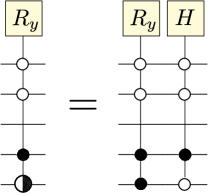
Figure 4: Definition of halfmoon vertices used in Fig.5.

4.1 Unordered Modular Models

In this section, we present one possible method for calculating $P({\cal F}|D)$ for unordered modular models, where $P({\cal F}|D)$ is given by Eq.(34).

One possible method of doing this is as follows: for each $j\in\{0..n-1\}$, calculate $\sum_{pa_{j}\subset{\left\{<j\right\}}}$ using the technique of Ref.[9] for calculating Mobius transforms.

4.2 Ordered Modular Models

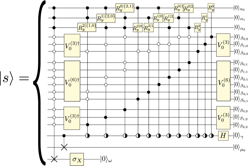
Figure 5: Circuit for generating $|s\rangle$ used in AFGA to calculate $\overline{P}({\cal F}|D)$ for ordered modular model. The $V_{0}^{(\lambda)}$ matrices are defined in Ref.[8].

In this section, we present one possible method for calculating $\overline{P}({\cal F}|D)$ for ordered modular models, where $\overline{P}({\cal F}|D)$ is given by Eq.(51). Eq.(51) is just a sum over all permutations in $Sym_{n}$. We have already shown how to do sums over permutations in Ref.[8]. So we could consider our job already done. However, using the method of Ref.[8] would entail the non-trivial task of finding a way of compiling the argument under the sum over permutations, a complicated $n$-fold product of $h()$ functions. In this section, we will give a method for calculating Eq.(51) that does not require compiling this $n$-fold product of $h()$ functions.

For each $j\in{\left\{0..n-1\right\}}$ and $S\subset\{0..n-1\backslash j\}$, define

$$h(j|S)=\sin(\theta_{j|S})\;$$ (54)

and

$$R_{y}^{j|S}=\exp(-i\sigma_{Y}\theta_{j|S})\;.$$ (55)

Let $|S|=\ell$. Define

$$N_{2}(\beta_{;\ell})=n\left(\begin{array}[]{c}n-1\\ \ell\end{array}\right)\;$$ (56)

and

$$N_{2}(\beta)=\sum_{\ell=0}^{n-1}N_{2}(\beta_{;\ell})=n2^{n-1}\;.$$ (57)

The following fraction will also come into play:

$$\epsilon=\frac{1}{\prod_{\ell=0}^{n-1}N_{2}(\beta_{;\ell})}\;.$$ (58)

We will use qubits $\beta_{c;\ell}$ for $c\in{\left\{0..N_{2}(\beta_{;\ell})-1\right\}}$ and $\ell\in{\left\{0..n-1\right\}}$. Let $\beta_{;\ell}=(\beta_{c;\ell})_{\forall c}$ and $\beta=(\beta_{;\ell})_{\forall\ell}$.

For concreteness, we will use $n=3$ henceforth in this section, but it will be obvious how to draw an analogous circuit for arbitrary $n$.

We want all horizontal lines in Fig.5 to represent qubits. Let $\alpha=\alpha^{3}$ and $\beta=(\beta_{;0},\beta_{;1},\beta_{;2})=(\beta^{3}_{;0},\beta^{6}_{;1},\beta^{3}_{;2})=\beta^{12}$.

Define

$$T_{x}(\alpha)=\epsilon\sum_{j_{0}=0}^{2}\sum_{j_{1}=0}^{2}\theta(j_{1}\neq j_{0})\sum_{j_{2}=0}^{2}\theta(j_{2}\neq j_{1},j_{2}\neq j_{0})T_{x}[j_{2},2](\alpha)T_{x}[j_{1},1](\alpha)T_{x}[j_{0},0](\alpha)\;$$ (59)

for $x=0,1$, where

$$T_{1}[j,\ell](\alpha)=\prod_{S\in{\left\{S:S\subset{\left\{0..n-1\backslash j\right\}},|S|=\ell\right\}}}[e^{-i\sigma_{Y}(\alpha_{j})\theta_{j|S}}]^{\prod_{k\in S}P_{1}(\alpha_{k})}\;$$ (60)

and

$$T_{0}[j,\ell](\alpha)=\prod_{S\in{\left\{S:S\subset{\left\{0..n-1\backslash j\right\}},|S|=\ell\right\}}}[H(\alpha_{j})]^{\prod_{k\in S}P_{1}(\alpha_{k})}\;$$ (61)

where $H(\alpha_{j})$ is a Hadamard matrix acting on bit $\alpha_{j}$. Also define

$$\pi(\alpha)=\prod_{j=0}^{2}P_{1}(\alpha_{j})\;,$$ (62)

and

$$\pi(\beta)=\left\{\begin{array}[]{l}\prod_{c=0}^{2}P_{0}(\beta_{c;0})\\ \prod_{c=0}^{5}P_{0}(\beta_{c;1})\\ \prod_{c=0}^{2}P_{0}(\beta_{c;2})\end{array}\right.\;.$$ (63)

Our method for calculating $\overline{P}({\cal F}|D)$ consists of applying the algorithm AFGA of Ref.[10] in the way that was described in Ref.[8], using the techniques of targeting two hypotheses and blind targeting. As in Ref.[8], when we apply AFGA in this section, we will use a sufficient target $|0\rangle_{\omega}$. All that remains for us to do to fully specify our circuit for calculating $\overline{P}({\cal F}|D)$ is to give a circuit for generating $|s\rangle$.

See Fig.4 where a halfmoon vertex that we will use in the next figure is defined. Controlled gates with one of these halfmoon vertices at the bottom should be interpreted as two gates, one with a $P_{0}$ control replacing the halfmoon, and one with a $P_{1}$ control replacing it. The one with the $P_{1}$ control should have at the top a $R_{y}$ rotation and the one with the $P_{0}$ control should have at the top a Hadamard matrix. All controls acting on qubits other than the qubits at the very top and very bottom are kept the same.

A circuit for generating $|s\rangle$ is given by Fig.5. The $V_{0}^{(\lambda)}$ matrices used in Fig.5. are defined in Ref.[8]. Fig.5 is equivalent to saying that

$$|s\rangle_{\mu,\nu,\omega}=\sigma_{X}(\omega)^{\pi(\beta)\pi(\alpha)}\frac{1}{\sqrt{2}}\left[\begin{array}[]{l}T_{1}(\alpha)|0^{3}\rangle_{\alpha}\\ |0^{12}\rangle_{\beta}\\ |1\rangle_{\gamma}\\ |1\rangle_{\mu_{0}}\\ |1\rangle_{\omega}\end{array}+\begin{array}[]{l}T_{0}(\alpha)|0^{3}\rangle_{\alpha}\\ |0^{12}\rangle_{\beta}\\ |0\rangle_{\gamma}\\ |0\rangle_{\mu_{0}}\\ |1\rangle_{\omega}\end{array}\right]\;.$$ (64)

Claim 1

$$|s\rangle_{\mu,\nu,\omega}=\begin{array}[]{c}z_{1}|\psi_{1}\rangle_{\mu}\\ |1\rangle_{\nu}\\ |0\rangle_{\omega}\end{array}+\begin{array}[]{c}z_{0}|\psi_{0}\rangle_{\mu}\\ |0\rangle_{\nu}\\ |0\rangle_{\omega}\end{array}+\begin{array}[]{c}|\chi\rangle_{\mu,\nu}\\ |1\rangle_{\omega}\end{array}\;,$$ (65)

for some unnormalized state $|\chi\rangle_{\mu,\nu}$, where

$$\begin{array}[]{|c|c|}\hline\cr|\psi_{1}\rangle_{\mu}=\begin{array}[]{l}|1^{3}\rangle_{\alpha}\\ |1\rangle_{\mu_{0}}\end{array}&|\psi_{0}\rangle_{\mu}=\begin{array}[]{l}|1^{3}\rangle_{\alpha}\\ |0\rangle_{\mu_{0}}\end{array}\\ |1\rangle_{\nu}=\left[\begin{array}[]{r}|0^{3}\rangle_{\beta_{;0}}\\ |0^{6}\rangle_{\beta_{;1}}\\ |0^{3}\rangle_{\beta_{;2}}\\ |1\rangle_{\gamma}\end{array}\right]&|0\rangle_{\nu}=\left[\begin{array}[]{r}|0^{3}\rangle_{\beta_{;0}}\\ |0^{6}\rangle_{\beta_{;1}}\\ |0^{3}\rangle_{\beta_{;2}}\\ |0\rangle_{\gamma}\end{array}\right]\\ \hline\cr\end{array}\;,$$ (66)

$$z_{1}=\frac{\epsilon}{\sqrt{2}}\sum_{\sigma}\overbrace{\left\{\sin(\theta_{2^{\sigma}|\{1^{\sigma},0^{\sigma}\}})\sin(\theta_{1^{\sigma}|0^{\sigma}})\sin(\theta_{0^{\sigma}})\right\}}^{=h_{2^{\sigma}|\{1^{\sigma},0^{\sigma}\}}h_{1^{\sigma}|0^{\sigma}}h_{0^{\sigma}}}\;,$$ (67a)

$$z_{0}=\frac{\epsilon n!}{\sqrt{2^{n+1}}}\;,$$ (67b)

$$\frac{|z_{1}|}{|z_{0}|}=\sqrt{\frac{P(1)}{P(0)}}\;.$$ (68)

proof:

Recall that for any quantum systems $\alpha$ and $\beta$, any unitary operator $U(\beta)$ and any projection operator $\pi(\alpha)$, one has

$$U(\beta)^{\pi(\alpha)}=(1-\pi(\alpha))+U(\beta)\pi(\alpha)\;.$$ (69)

Applying identity Eq.(69) with $U=\sigma_{X}(\omega)$ yields:

$$|s\rangle = \sigma_{X}(\omega)^{\pi(\beta)\pi(\alpha)}|s^{\prime}\rangle$$ (70)

$$= \sigma_{X}(\omega)\pi(\beta)\pi(\alpha)|s^{\prime}\rangle+\begin{array}[]{l}|\chi\rangle_{\mu,\nu}\\ |1\rangle_{\omega}\end{array}\;.$$ (73)

Note that $T_{1}(\alpha)$ is a sum of $n^{n}$ terms, which is more than $n!$ terms, but the controls in those $n^{n}$ terms together with the act of taking the matrix element between $\langle 1^{3}|$ and $|0^{3}\rangle$, reduces the number of summed over terms to $n!$:

$$\langle 1^{3}|T_{1}(\alpha)|0^{3}\rangle = \epsilon\sum_{\sigma\in Sym_{n}}\langle 1^{3}|\begin{array}[]{r}\exp\left[-i\sigma_{Y}(\alpha_{2^{\sigma}})\theta_{2^{\sigma}|\{1^{\sigma},0^{\sigma}\}}\right]\\ \exp\left[-i\sigma_{Y}(\alpha_{1^{\sigma}})\theta_{1^{\sigma}|0^{\sigma}}\right]\\ \exp\left[-i\sigma_{Y}(\alpha_{0^{\sigma}})\theta_{0^{\sigma}}\right]\end{array}|0^{3}\rangle$$ (77)

$$= \epsilon\sum_{\sigma}\begin{array}[]{r}\sin(\theta_{2^{\sigma}|{\left\{1^{\sigma},0^{\sigma}\right\}}})\\ \sin(\theta_{1^{\sigma}|0^{\sigma}})\\ \sin(\theta_{0^{\sigma}})\end{array}\;.$$ (81)

Likewise,

$$\langle 1^{3}|T_{0}(\alpha)|0^{3}\rangle = \epsilon\sum_{\sigma\in Sym_{n}}\langle 1^{3}|H(\alpha_{2})H(\alpha_{1})H(\alpha_{0})|0^{3}\rangle$$ (82)

$$= \frac{\epsilon n!}{\sqrt{2^{n}}}\;.$$ (83)

QED

To draw the circuit of Fig.5, especially for $n$ much larger than 3, requires that one know how to enumerate all possible combinations of $\ell$ elements from a set of $n$ elements. A simple algorithm for doing this is known (Ref.[14]). It’s based on a careful study of the pattern in simple examples such as this one:

Choose 3 elements out of the set $\{0,1,2,3,4\}$:

$$\begin{array}[]{|c|c|c|c|c|}\hline\cr 0&1&2&&\\ \hline\cr 0&1&&3&\\ \hline\cr 0&1&&&4\\ \hline\cr 0&&2&3&\\ \hline\cr 0&&2&&4\\ \hline\cr 0&&&3&4\\ \hline\cr&1&2&3&\\ \hline\cr&1&2&&4\\ \hline\cr&1&&3&4\\ \hline\cr&&2&3&4\\ \hline\cr\end{array}\;$$ (84)

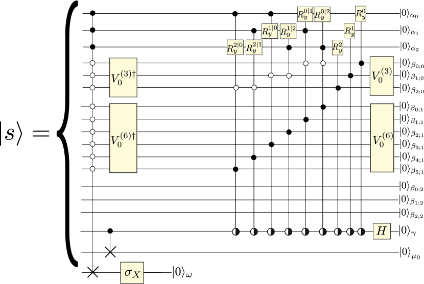
Figure 6: Circuit for generating $|s\rangle$ used in AFGA to calculate $\overline{P}({\cal F}|D)$ for ordered modular model. This is a simplification of Fig.5, assuming that the in-degree of all nodes is smaller or equal to one.

A more serious problem with using the circuit of Fig.5 for large $n$ is that as Eq.(57) indicates, the number of $\beta$ qubits grows exponentially with $n$ so the circuit Fig.5 is too expensive for large $n$’s. However, one can make an assumption which doesn’t seem too restrictive, namely that the in-degree (number of parent nodes) $\ell$ of all nodes of the graph $G$ is $\leq\ell_{max}$, where the bound $\ell_{max}$ does not grow with $n$. Define

$$N_{2}^{\prime}(\beta)=\sum_{\ell=0}^{\ell_{max}}N_{2}(\beta_{;\ell})={\cal O}(n)\;$$ (85)

and

$$\epsilon^{\prime}=\frac{1}{\prod_{\ell=0}^{\ell_{max}}N_{2}(\beta_{;\ell})}\;.$$ (86)

The order estimate for $N^{\prime}_{2}(\beta)$ given by Eq.(85) can be proven using Stirling’s approximation.

For example, consider Fig.5. If $\ell\leq\ell_{max}=1$ for that figure, then we can omit all the $\beta_{;2}$ qubits, and the $R_{y}^{a|{\left\{b,c\right\}}}$ rotations for $a,b,c\in{\left\{0,1,2\right\}}$. In other words, Fig.5 can be simplified to Fig.6. Claim 1 still holds if we replace $h(2^{\sigma}|\{1^{\sigma},0^{\sigma}\})$ by 1 and $\epsilon$ by $\epsilon^{\prime}$ in Eqs.(67).

References

- [1] G.F. Cooper, and E. Herskovits, “A Bayesian method for the induction of probabilistic networks from data”, Machine learning 9.4 (1992): 309-347.
- [2] N. Friedman, and D. Koller, “Being Bayesian about network structure. A Bayesian approach to structure discovery in Bayesian networks”, Machine learning 50.1-2 (2003): 95-125.
- [3] M. Koivisto, and K. Sood, “Exact Bayesian structure discovery in Bayesian networks”, The Journal of Machine Learning Research 5 (2004): 549-573.
- [4] M. Koivisto, “Advances in exact Bayesian structure discovery in Bayesian networks”, arXiv:1206.6828
- [5] B. Ellis, and Wing Hung Wong, “Learning causal Bayesian network structures from experimental data”, Journal of the American Statistical Association 103.482 (2008).
- [6] is Ru He, Jian Tian, “Bayesian Learning in Bayesian Networks of Moderate Size by Efficient Sampling”. Unpublished.
- [7] R.R. Tucci, “Quibbs, a Code Generator for Quantum Gibbs Sampling”, arXiv:1004.2205
- [8] R.R. Tucci, “Quantum Circuit for Calculating Symmetrized Functions Via Grover-like Algorithm”, arXiv:1403.6707
- [9] R.R. Tucci, “Quantum Circuit for Calculating Mobius-like Transforms Via Grover-like Algorithm”, arXiv:1403.6910
- [10] R.R. Tucci, “An Adaptive, Fixed-Point Version of Grover’s Algorithm”, arXiv:1001.5200
- [11] D-Wave/Google image classification papers
- [12] P. Rebentrost, M. Mohseni, and S. Lloyd, “Quantum support vector machine for big feature and big data classification”, arXiv:1307.0471
- [13] N. Wiebey, A. Kapoor, and K. Svore, “Quantum Nearest-Neighbor Algorithms for Machine Learning”, arXiv:1401.2142
- [14] Bryan Flamig, Practical Algorithms in C++, (John Wiley & Sons, 1995)