A fast multipole method for the evaluation of elastostatic fields in a half-space with zero normal stress

Abstract

In this paper, we present a fast multipole method (FMM) for the half-space Green’s function in a homogeneous elastic half-space subject to zero normal stress, for which an explicit solution was given by Mindlin (1936). The image structure of this Green’s function is unbounded, so that standard outgoing representations are not easily available. We introduce two such representations here, one involving an expansion in plane waves and one involving a modified multipole expansion. Both play a role in the FMM implementation.

Key words. Fast multipole method; Linear elasticity; Mindlin’s solution.

1 Introduction

A classical problem in linear elasticity concerns the computation of the displacement, stress and strain due to force and dislocation sources with suitable boundary conditions imposed on a half-space. The case of zero normal stress is of particular importance in geophysical applications, for which the exact solution was derived by Mindlin [11].

We will concentrate here on the question of accelerating the evaluation of the field due to a collection of such force and dislocation vectors. More precisely, we will describe two new analytic representations for the image structure in Mindlin’s solution that can be incorporated into a fast multipole method (FMM). With $N$ sources and $M$ sensor/target locations, the FMM reduces the cost of evaluating the fields from $O(NM)$ to $O(N+M)$. The FMM can also be used to accelerate integral-equation based methods for elastostatic boundary value problems on surfaces embedded in the half-space, avoiding the ill-conditioning associated with finite element and finite difference discretizations of the underlying partial differential equations.

We will begin with a discussion of the mathematical foundations for the new scheme, followed by a brief description of the full FMM implementation. For readers unfamiliar with fast multipole methods, we suggest the papers [1, 8] to gain some familiarity, although the mathematical treatment here is largely self-contained.

In section 6, we present numerical experiments both for collections of singular sources and for the evaluation of layer potentials using the quadrature method of [6].

2 The Mindlin solution

To fix notation, let us first consider the displacement at an observation point $(x_{1},x_{2},x_{3})$ due to a force vector ${\bf F}=(F_{1},F_{2},F_{3})$ acting at the source point $(\xi_{1},\xi_{2},\xi_{3})$ in free-space. The solution is given by the well-known Kelvin solution:

$${u_{i}}={K_{i}^{j}}F_{j}\,,$$

where

$${K_{i}^{j}}=\frac{1}{8\pi\mu}\left\{(2-\alpha)\frac{\delta_{ij}}{r}+\alpha\frac{(x_{i}-\xi_{i})(x_{j}-\xi_{j})}{r^{3}}\right\}\,,$$ (1)

$r=\sqrt{(x_{1}-\xi_{1})^{2}+(x_{2}-\xi_{2})^{2}+(x_{3}-\xi_{3})^{2}}$, $\alpha=(\lambda+\mu)/(\lambda+2\mu)$, and $\lambda,\mu$ are the Lamé coefficients. (In the preceding expressions, and throughout the paper, we will generally make use of the standard summation convention. On occasion we will write out the formulas explicitly when it makes the analysis clearer.)

Formulas for the strain ${\varepsilon_{ij}}$ and stress ${\sigma_{ij}}$ tensors can be obtained from partial derivatives of the preceding formulas for displacement with respect to each component $x_{i}$:

$${\varepsilon_{ij}}=\frac{1}{2}\left(\frac{\partial{u_{i}}}{\partial x_{j}}+\frac{\partial{u_{j}}}{\partial x_{i}}\right)\,,$$ (2)

$${\sigma_{ij}}=\lambda\delta_{ij}\frac{\partial{u_{n}}}{\partial x_{n}}+\mu\left(\frac{\partial{u_{i}}}{\partial x_{j}}+\frac{\partial{u_{j}}}{\partial x_{i}}\right)\,.$$ (3)

A number of fast methods for the Kelvin solution have been developed, based either on the FFT or the FMM [2, 3, 9, 21, 14, 15, 16, 20].

In a half-space, the solution is more complicated, involving several image sources. We assume that the $x_{3}$-axis points up and that sources $Q=(\xi_{1},\xi_{2},\xi_{3})$ and targets $P=(x_{1},x_{2},x_{3})$ are in the lower half-space ($x_{3},\xi_{3}<0$). With a slight modification of Okada’s notation [13], we let

$$R_{1}=x_{1}-\xi_{1}\ ,\ R_{2}=x_{2}-\xi_{2}\ ,\ R_{3}=-(x_{3}+\xi_{3}),$$

corresponding to the usual Cartesian components of the vector from the image source $(\xi_{1},\xi_{2},-\xi_{3})$ to the target, with the sign flipped in the $R_{3}$ component. Note that $R_{3}\geq 0$. We denote the distance from the image to the target point by

$$R=\sqrt{R_{1}^{2}+R_{2}^{2}+R_{3}^{2}}\,.$$

Mindlin showed that the exact solution to the half-space problem with zero normal stress can be written in the form $u_{i}=W_{i}^{j}F_{j}$, where

$$W_{i}^{j}(P,Q)=\ {K_{i}^{j}}(P,Q)+{A_{i}^{j}}(P,Q)$$

$$+{B_{i}^{j}}(P,Q)+x_{3}{C_{i}^{j}}(P,Q),$$ (4)

with

$${A_{i}^{j}}= \frac{1}{8\pi\mu}\left\{\alpha\frac{\delta_{ij}}{R}+(2-\alpha)\frac{R_{i}R_{j}}{R^{3}}\right\}\,,$$ (5)

$${B_{i}^{j}}= \frac{1}{4\pi\mu}\left\{\frac{1-\alpha}{\alpha}\left[\frac{\delta_{ij}}{R+R_{3}}+\frac{R_{i}\delta_{j3}-R_{j}\delta_{i3}(1-\delta_{j3})}{R(R+R_{3})}\right.\right.$$

$$\left.\left.-\frac{R_{i}R_{j}}{R(R+R_{3})^{2}}(1-\delta_{i3})(1-\delta_{j3})\right]\right\}\,,$$ (6)

$${C_{i}^{j}}= \frac{1}{4\pi\mu}(1-2\delta_{i3})\left\{(2-\alpha)\frac{R_{i}\delta_{j3}-R_{j}\delta_{i3}}{R^{3}}+\right.$$

$$\left.\quad\alpha\xi_{3}\left[\frac{\delta_{ij}}{R^{3}}-\frac{3R_{i}R_{j}}{R^{5}}\right]\right\}.$$ (7)

Definition 1.

We will refer to $W_{i}^{j}$ as the single-layer kernel in a half-space.

The first contribution to ${W_{i}^{j}}$ in formula (4) is the “direct arrival” from the source in a uniform infinite medium, given by the Kelvin formula (1). The second piece ${A_{i}^{j}}$ has the same form, but with the roles of $\alpha$ and $(2-\alpha)$ reversed. Since $R_{3}=-x_{3}-\xi_{3}$, this is the arrival at “target” $(x_{1},x_{2},-x_{3})$ from a source at $(\xi_{1},\xi_{2},\xi_{3})$ with modified Lamé coefficients. Thus, interactions governed by both the $K_{i}^{j}$ and $A_{i}^{j}$ contributions can be computed using the “free-space” single-layer kernel. ${B_{i}^{j}}$ and ${C_{i}^{j}}$ are quite different and their analysis is the principal contribution of this paper.

Remark 2.

A simple algebraic trick permits the computation of the $A_{i}^{j}$ contributions. Namely, we set ${\tilde{\lambda}}=\lambda+4\mu$ and ${\tilde{\mu}}=-\mu$. It is easy to check that

$${\tilde{\alpha}}=({\tilde{\lambda}}+{\tilde{\mu}})/({\tilde{\lambda}}+2{\tilde{\mu}})=(2-\alpha),\quad(2-{\tilde{\alpha}})=\alpha\,.$$

Thus,

$${A_{i}^{j}}(x_{1},x_{2},x_{3})={K_{i}^{j}}[{\tilde{\lambda}},{\tilde{\mu}}](x_{1},x_{2},-x_{3})\,,$$

where $K_{i}^{j}[{\tilde{\lambda}},{\tilde{\mu}}]$ denotes the Kelvin formula with the dependence on the Lamé coefficients made explicit.

Remark 3.

Note that the argument $x_{3}$ has been replaced by $-x_{3}$, so that some care is required when evaluating terms such as $\partial u_{i}/\partial x_{l}$ which appear in the stress and strain tensors.

Definition 4.

The double-layer kernel in a half-space is given by

$$T_{i}^{j}=\left[\lambda\delta_{jk}\frac{\partial W_{i}^{n}}{\partial{\xi_{n}}}+\mu\left(\frac{\partial W_{i}^{j}}{\partial{\xi_{k}}}+\frac{\partial W_{i}^{k}}{\partial{\xi_{j}}}\right)\right]\nu_{k}.$$ (8)

This kernel describes the displacement field due to a dislocation vector ${\bf D}=(D_{1},D_{2},D_{3})$ across a surface $S$ with orientation vector ${\bf{\boldsymbol{\nu}}}=(\nu_{1},\nu_{2},\nu_{3})$:

$$u_{i}=\int\int_{S}T_{i}^{j}D_{j}\,dS\,.$$ (9)

(Typically, the orientation vector is normal to the surface $S$.) The dislocation vector ${\bf D}$ is sometimes called a double-force vector.

To compute $T_{i}^{j}$, we note first that

$$\frac{\partial u_{i}^{j}}{\partial\xi_{k}}(x_{1},x_{2},x_{3})= \frac{\partial{K_{i}^{j}}}{\partial\xi_{k}}(x_{1},x_{2},x_{3})+\frac{\partial{A_{i}^{j}}}{\partial\xi_{k}}(x_{1},x_{2},x_{3})$$

$$+\frac{\partial{B_{i}^{j}}}{\partial\xi_{k}}(x_{1},x_{2},x_{3})+x_{3}\frac{\partial{C_{i}^{j}}}{\partial\xi_{k}}(x_{1},x_{2},x_{3}),$$ (10)

where [11, 13, 17]

$$\frac{\partial{K_{i}^{j}}}{\partial\xi_{k}} =\frac{1}{8\pi\mu}\left\{(2-\alpha)\frac{(x_{k}-\xi_{k})}{r^{3}}\delta_{ij}-\alpha\frac{(x_{i}-\xi_{i})\delta_{jk}+(x_{j}-\xi_{j})\delta_{ik}}{r^{3}}\right.$$

$$\left.\qquad+3\alpha\frac{(x_{i}-\xi_{i})(x_{j}-\xi_{j})(x_{k}-\xi_{k})}{r^{5}}\right\}\,,$$ (11)

$$\frac{\partial{A_{i}^{j}}}{\partial\xi_{k}} =\frac{1}{8\pi\mu}\left\{\alpha\frac{R_{k}}{R^{3}}\delta_{ij}-(2-\alpha)\frac{R_{i}\delta_{jk}+R_{j}\delta_{ik}}{R^{3}}+3(2-\alpha)\frac{R_{i}R_{j}R_{k}}{R^{5}}\right\},$$ (12)

$$\frac{\partial{B_{i}^{j}}}{\partial\xi_{k}} =\frac{1}{4\pi\mu}\left\{-\frac{R_{i}\delta_{jk}+R_{j}\delta_{ik}-R_{k}\delta_{ij}}{R^{3}}+\frac{3R_{i}R_{j}R_{k}}{R^{5}}\right.$$

$$\qquad+\frac{1-\alpha}{\alpha}\left[\frac{\delta_{3k}R+R+k}{R(R+R_{3})^{2}}\delta_{ij}-\frac{\delta{ik}\delta_{j3}-\delta_{jk}\delta_{i3}(1-\delta_{j3})}{R(R+R_{3})}\right.$$

$$\qquad+[R_{i}\delta_{j3}-R_{j}\delta_{i3}(1-\delta_{j3})]\frac{\delta_{3k}R^{2}+R_{k}(2R+R_{3})}{R^{3}(R+R_{3})^{2}}$$ (13)

$$\qquad+\left[\frac{R_{i}\delta_{jk}+R_{j}\delta_{ik}}{R(R+R_{3})^{2}}-\right.$$

$$\qquad\qquad\left.\left.\left.R_{i}R_{j}\frac{2\delta_{3k}R^{2}+R_{k}(3R+R_{3})}{R^{3}(R+R_{3})^{3}}\right](1-\delta_{i3})(1-\delta_{j3})\right]\right\},$$

$$\frac{\partial{C_{i}^{j}}}{\partial\xi_{k}} =\frac{1}{4\pi\mu}(1-2\delta_{i3})\left\{(2-\alpha)\left[\frac{\delta_{jk}\delta_{i3}-\delta_{ik}\delta_{j3}}{R^{3}}+\right.\right.$$

$$\qquad\qquad\left.\frac{3R_{k}(R_{i}\delta_{j3}-R_{j}\delta_{i3})}{R^{5}}\right]+\alpha\left[\frac{\delta_{ij}}{R^{3}}-\frac{3R_{i}R_{j}}{R^{5}}\right]\delta_{3k}+$$ (14)

$$\qquad\qquad\left.3\alpha\xi_{3}\left[\frac{R_{i}\delta_{jk}+R_{j}\delta_{ik}+R_{k}\delta_{ij}}{R^{5}}-\frac{5R_{i}R_{j}R_{k}}{R^{7}}\right]\right\}.$$

As for the single-layer kernel,

$$\frac{\partial{A_{i}^{j}}}{\partial\xi_{k}}(x_{1},x_{2},x_{3})=\frac{\partial{K_{i}^{j}}}{\partial\xi_{k}}[{\tilde{\lambda}},{\tilde{\mu}}](x_{1},x_{2},-x_{3})\,.$$

We need to compute the contribution of $A_{i}^{j}$ to the double-layer kernel $T_{i}^{j}$ according to (8):

$$u_{i}=\left[\lambda\delta_{jk}\frac{\partial{A_{i}^{n}}}{\partial\xi_{n}}+\mu\left(\frac{\partial{A_{i}^{j}}}{\partial\xi_{k}}+\frac{\partial{A_{i}^{k}}}{\partial\xi_{j}}\right)\right]\nu_{k}D_{j}\,.$$

Suppose that we invoke the free-space double-layer kernel with ${\tilde{\lambda}},{\tilde{\mu}}$ and dislocation vector $-{\bf D}$, so that we actually compute

$$u_{i}^{*} =\left[-{\tilde{\lambda}}\delta_{jk}\frac{\partial{A_{i}^{n}}}{\partial\xi_{n}}-{\tilde{\mu}}\left(\frac{\partial{A_{i}^{j}}}{\partial\xi_{k}}-\frac{\partial{A_{i}^{k}}}{\partial\xi_{j}}\right)\right]\nu_{k}D_{j}$$

$$=\left[-{\tilde{\lambda}}\delta_{jk}\frac{\partial{A_{i}^{n}}}{\partial\xi_{n}}+\mu\left(\frac{\partial{A_{i}^{j}}}{\partial\xi_{k}}+\frac{\partial{A_{i}^{k}}}{\partial\xi_{j}}\right)\right]\nu_{k}D_{j}\,.$$

Fortunately, the difference is a simple harmonic function:

$$u_{i}-u_{i}^{*} =\left[({\tilde{\lambda}}+\lambda)\delta_{jk}\frac{\partial{A_{i}^{n}}}{\partial\xi_{n}}\right]\nu_{k}D_{j}$$

$$=({\tilde{\lambda}}+\lambda)\frac{\partial{A_{i}^{n}}}{\partial\xi_{n}}({\bf{\boldsymbol{\nu}}\cdot{D}})$$

$$=\frac{1}{8\pi\mu}(2\lambda+4\mu)({\bf{\boldsymbol{\nu}}\cdot{D}})\left\{\alpha\frac{R_{i}}{R^{3}}-(2-\alpha)\frac{3R_{i}+R_{i}}{R^{3}}+3(2-\alpha)\frac{R_{i}R^{2}}{R^{5}}\right\}$$

$$=\frac{1}{8\pi\mu}(2\lambda+4\mu)({\bf{\boldsymbol{\nu}}\cdot{D}})(2\alpha-2)\frac{R_{i}}{R^{3}}$$

$$=\frac{1}{2\pi}({\bf{\boldsymbol{\nu}}\cdot{D}})\frac{-R_{i}}{R^{3}}=\frac{1}{2\pi}({\bf{\boldsymbol{\nu}}\cdot{D}})\frac{\partial}{\partial x_{i}}\frac{1}{R}\,.$$ (15)

This difference can be computed using a single call to the FMM for the Laplace equation, since the result is simply the gradient of the field due to a point source with strength $({\bf{\boldsymbol{\nu}}\cdot{D}})$.

Remark 5.

For those keeping careful track of indices, note that, using the Okada notation, it is indeed the gradient that is required. We have moved $x_{3}$ to $-x_{3}$ in the free space call. Thus,

$$\frac{\partial}{\partial x_{3}}\frac{1}{R}=-(-x_{3}-\xi_{3})/R^{3}=(x_{3}+\xi_{3})/R^{3}=-R_{3}/R^{3}\,,$$

justifying the last equality in (15).

The difficulty in developing a fast algorithm for the Mindlin solution, however, lies not in handling the free space kernel $K_{i}^{j}$ or the simple image $A_{i}^{j}$. Rather, it lies in the kernels $B_{i}^{j}$ and $C_{i}^{j}$.

3 The $B$ image

Ignoring the scaling factor $\frac{1}{4\pi\mu}\,\frac{1-\alpha}{\alpha}$, the components of displacement induced by the $B$ image can be written in the form:

$$u_{i}^{B}=\frac{F_{i}}{R+R_{3}}+\frac{R_{i}F_{3}}{R(R+R_{3})}-\frac{\delta_{i3}(F_{1}R_{1}+F_{2}R_{2})}{R(R+R_{3})}-\frac{R_{i}(1-\delta_{i3})(F_{1}R_{1}+F_{2}R_{2})}{R(R+R_{3})^{2}}.$$

Without entering into a detailed derivation, Mindlin’s basic observation was that the $B$ image could be derived from a consideration of all second derivatives of a scalar potential. More precisely, we have the following lemma.

Lemma 6.

Let ${\cal B}(R_{1},R_{2},R_{3})$ denote the scalar potential given by ${\cal B}(R_{1},R_{2},R_{3})=R_{3}\log(R+R_{3})-R$. Then

$${\cal B}_{1}=\frac{-R_{1}}{R+R_{3}},\qquad{\cal B}_{2}=\frac{-R_{2}}{R+R_{3}},\qquad{\cal B}_{3}=\log(R+R_{3}),$$

$${\cal B}_{11} =\frac{-1}{R+R_{3}}+\frac{R_{1}^{2}}{R(R+R_{3})^{2}},\qquad{\cal B}_{12}=\frac{R_{1}R_{2}}{R(R+R_{3})^{2}},\qquad{\cal B}_{13}=\frac{R_{1}}{R(R+R_{3})},$$

$${\cal B}_{22} =\frac{-1}{R+R_{3}}+\frac{R_{2}^{2}}{R(R+R_{3})^{2}},\qquad{\cal B}_{23}=\frac{R_{2}}{R(R+R_{3})},\qquad{\cal B}_{33}=\frac{1}{R}\,,$$

where the subscript denotes differentiation with respect to the corresponding variable $R_{i}$. It follows that the contribution to the displacement induced by the $B$ image in the single-layer kernel is given by

$$(u_{1}^{B},u_{2}^{B},-u_{3}^{B})=\nabla_{\bf x}[(F_{1},F_{2},F_{3})\cdot\nabla_{\overline{\xi}}{\cal B}]\,,$$

where $\nabla_{\bf x}$ denotes the gradient with respect to the target location and $\nabla_{\overline{\xi}}$ denotes the gradient with respect to the image source location at $(\xi_{1},\xi_{2},-\xi_{3})$.

Remark 7.

Note that if ${\cal B}$ were the potential due to a simple charge source, then $(u_{1}^{B},u_{2}^{B},-u_{3}^{B})$ would be the gradient of the potential induced by a dipole with orientation and strength given by $(F_{1},F_{2},F_{3})$.

A straightforward but tedious calculation yields

Lemma 8.

Let ${\cal B}(R_{1},R_{2},R_{3})=R_{3}\log(R+R_{3})-R$. Then the contribution to the displacement induced by the $B$ image in the double-layer kernel is given by

$$(u_{1}^{B},u_{2}^{B},-u_{3}^{B})=\nabla_{\bf x}{\cal D}\,,$$

where

$${\cal D} =2\mu\left[F_{1}\nu_{1}{\cal B}_{\xi_{1}\xi_{1}}+F_{2}\nu_{2}{\cal B}_{\xi_{2}\xi_{2}}-F_{3}\nu_{3}{\cal B}_{\xi_{3}\xi_{3}}+(F_{2}\nu_{1}+F_{1}\nu_{2}){\cal B}_{\xi_{1}\xi_{2}}\right]$$

$$\qquad-2\lambda({\bf{\boldsymbol{\nu}}\cdot{F}}){\cal B}_{\xi_{3}\xi_{3}}.$$ (16)

Remark 9.

Note that the formula for ${\cal D}$ in Lemma 8 is, in essence, a quadrupole field of a ${\cal B}$-type source with specific second derivative contributions defined in (16).

3.1 Far field and local representations for the $B$ image

It is easy to verify that ${\cal B}$ is a scalar harmonic function in the lower half-space. It is also clear, however, that it cannot describe the field due to a bounded collection of charges, since ${\cal B}$ is growing as $R_{3}\rightarrow\infty$. In this section, we describe some new far field representations that are somewhat involved, but permit much more efficient computation.

Figure 1: The influence of the ${\cal B}$ (and ${\cal C}$) images in the boxes ${\bf s}_{1}$ and ${\bf s}_{2}$ needs to be computed at subsurface target locations in boxes ${\bf n}$ and ${\bf m}$. In the FMM, this can be accomplished using a local expansion in the target boxes, an outgoing expansion in the source boxes, or both.

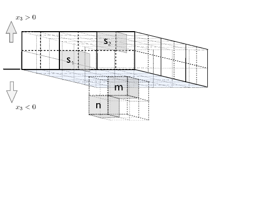
We begin by considering the ${\cal B}$-type sources contained in the boxes ${\bf s}_{1}$ and ${\bf s}_{2}$ in Fig. 1. They are separated from the target boxes ${\bf n}$ and ${\bf m}$ by at least one box length, so that far field and/or local expansions should be rapidly convergent. From above, the displacement in the lower half-space due to the image sources in, say, ${\bf s}_{1}$ is given by $(u_{1}^{B},u_{2}^{B},-u_{3}^{B})=\nabla_{\bf x}\Phi_{{\cal B}}$, where the scalar $\Phi_{{\cal B}}$ is given by

$$\Phi_{{\cal B}}=\sum_{n=1}^{N}{\bf F}^{(n)}\cdot\nabla_{\overline{\xi}}{\cal B}(R^{(n)}_{1},R^{(n)}_{2},R^{(n)}_{3}),$$ (17)

where $N$ denotes the number of image sources in ${\bf s}_{1}$ and $(R^{(n)}_{1},R^{(n)}_{2},R^{(n)}_{3})$ denotes the vector from the $n$th image source to the target point ${\bf x}=(x_{1},x_{2},x_{3})$.

Within the box ${\bf n}$, however, the field $\Phi_{{\cal B}}$ is smooth and harmonic, and can be written in the form of a local expansion:

$$\Phi_{{\cal B}}({\bf x})\approx\sum_{n=0}^{p}\sum_{m=-n}^{n}L_{n}^{m}\,Y_{n}^{m}(\theta,\phi)\,r^{n},$$ (18)

with $(r,\theta,\phi)$ the spherical coordinates of ${\bf x}$ with respect to the box center of ${\bf n}$. Here, $Y_{n}^{m}$ is the usual spherical harmonic of degree $n$ and order $m$

$$Y_{n}^{m}(\theta,\phi)=\sqrt{\frac{2n+1}{4\pi}}\sqrt{\frac{(n-|m|)!}{(n+|m|)!}}\,P_{n}^{|m|}(\cos\theta)e^{im\phi},$$ (19)

where the associated Legendre functions $P_{n}^{m}$ are defined by the Rodrigues’ formula

$$P_{n}^{m}(x)=(-1)^{m}(1-x^{2})^{m/2}\frac{d^{m}}{dx^{m}}P_{n}(x),$$

and $P_{n}(x)$ is the Legendre polynomial of degree $n$.

The coefficients of the local expansion can be computed by projection onto the spherical harmonic basis (integrating over the surface of a sphere enclosing the box ${\bf n}$ and centered at the box center). That is,

$$L_{n}^{m}=r^{-n}\,\int_{0}^{\pi}\int_{0}^{2\pi}Y_{n}^{-m}(\theta,\phi)\Phi_{{\cal B}}(r,\theta,\phi)\,d\phi\,d\theta.$$ (20)

This can be carried out in $O(p^{3})$ work, where $p$ is the order of the expansion in (18) by using a tensor product grid with $2p$ Gauss-Legendre nodes in the $\theta$ variable and $2p$ equispaced nodes in the $\phi$ variable.

In order to develop a more efficient fast algorithm, however, we would like to have outgoing representations from the source box ${\bf s}_{1}$ that can make use of the full framework of the FMM [1, 8]. One such representation is based on the plane wave formula ([12], p. 1256) for the potential at a target $(x_{1},x_{2},x_{3})$ due to a simple charge source at $(\xi_{1},\xi_{2},-\xi_{3})$:

$$\frac{1}{\sqrt{(x_{1}-\xi_{1})^{2}+(x_{2}-\xi_{2})^{2}+(x_{3}+\xi_{3})^{2}}}\hskip 108.405pt$$

$$=\frac{1}{2\pi}\int_{0}^{\infty}e^{\sigma(x_{3}+\xi_{3})}\int_{0}^{2\pi}e^{i\sigma((x_{1}-\xi_{1})\cos\alpha+(x_{2}-\xi_{2})\sin\alpha)}d\alpha\,d\sigma,$$ (21)

valid for $x_{3},\xi_{3}<0$.

The following theorem provides an expression for the displacement induced by single and double-layer sources in terms of plane waves (that is, complex exponentials of the components $(x_{1},x_{2},x_{3})$).

Theorem 10.

Let $(u_{1}^{B},u_{2}^{B},u_{3}^{B})$ denote the displacement induced by a single-layer force vector $(F_{1},F_{2},F_{3})$ located at the image source $(\xi_{1},\xi_{2},-\xi_{3})$ that lies in a source box ${\bf s}$ centered at $(S_{1},S_{2},S_{3})$. Then

$$u_{i}^{B}=\frac{1}{2\pi}\int_{0}^{\infty}{e^{\sigma(x_{3}-S_{3})}}\int_{0}^{2\pi}e^{i\sigma((x_{1}-S_{1})\cos\alpha+(x_{2}-S_{2})\sin\alpha)}M_{i}(\alpha)W(\sigma,\alpha)\,d\alpha\,d\sigma,$$

where

$$W(\sigma,\alpha)=\left(-F_{1}i\cos\alpha-F_{2}i\sin\alpha+F_{3}\right)e^{\sigma(i(S_{2}-\xi_{2})+i(S_{1}-\xi_{1})+(S_{3}+\xi_{3}))}$$

and

$$M_{1}(\alpha)=i\cos\alpha,\qquad M_{2}(\alpha)=i\sin\alpha,\qquad M_{3}(\alpha)=-1.$$ (22)

Theorem 10 can be proven by Fourier analysis and contour deformation, as in the derivation of the representation (21) in [12].

Remark 11.

Alternatively, we recall that ${\cal B}_{33}=\frac{1}{R}$. We may write this relation in the form

$${\cal B}=\partial_{x_{3}}^{-2}\left(\frac{1}{R}\right)\,.$$ (23)

It is straightforward to check that constants of integration can be ignored since they would only permit linear functions of $x_{1}$, $x_{2}$, and $x_{3}$ to appear in ${\cal B}$ and these are annihilated by the second derivative operators which arise in computing the displacement, according to Lemma 6. Note now that the operator $\partial_{x_{3}}^{-2}$ corresponds in (21) to division by $\sigma^{2}$. This results in a divergent integral, but using Lemma 6 again, the displacement clearly corresponds to multiplication by a factor of either $\sigma\cos\alpha$, $\sigma\sin\alpha$, or $\sigma$ (the signatures of $\partial_{x_{1}}$, $\partial_{x_{2}}$, and $\partial_{x_{3}}$, respectively). This argument, of course, is not entirely rigorous, but can be made so.

By superposition, we obtain a plane wave expansion for the field due to a set of sources, summarized in the following lemma.

Lemma 12.

Let $(u_{1}^{B},u_{2}^{B},u_{3}^{B})$ denote the displacement induced by a collection of single-layer force vectors $\{(F^{n}_{1},F^{n}_{2},F^{n}_{3}),n=1,\dots,N\}$ at image source locations

$$\{(\xi^{n}_{1},\xi^{n}_{2},-\xi^{n}_{3}),n=1,\dots,N\},$$

lying in a source box ${\bf s}$ centered at $(S_{1},S_{2},S_{3})$. Then the components of displacement are given by the plane wave representation of Theorem 10, with

$$W(\sigma,\alpha)=\sum_{n=1}^{N}\left(-F^{n}_{1}i\cos\alpha-F^{n}_{2}i\sin\alpha+F^{n}_{3}\right)e^{\sigma(i(S_{2}-\xi^{n}_{2})+i(S_{1}-\xi^{n}_{1})+(S_{3}+\xi^{n}_{3}))}.$$

A plane wave expansion can be obtained for the double-layer kernel as well. The proof is analogous.

Theorem 13.

Let $(u_{1}^{B},u_{2}^{B},u_{3}^{B})$ denote the displacement induced by a double-layer force vector ${\bf D}=(D_{1},D_{2},D_{3})$ with orientation vector ${\bf{\boldsymbol{\nu}}}=(\nu_{1},\nu_{2},\nu_{3})$, located at the image source $(\xi_{1},\xi_{2},-\xi_{3})$ that lies in a source box ${\bf s}$ centered at $(S_{1},S_{2},S_{3})$. Then,

$$u_{i}^{B}=\frac{1}{2\pi}\int_{0}^{\infty}{e^{\sigma(x_{3}-S_{3})}}\int_{0}^{2\pi}e^{i\sigma((x_{1}-S_{1})\cos\alpha+(x_{2}-S_{2})\sin\alpha)}M_{i}(\alpha)W(\sigma,\alpha)\,d\alpha\,d\sigma,$$

where

$$W(\sigma,\alpha) =\sigma e^{\sigma(i(S_{2}-\xi_{2})+i(S_{1}-\xi_{1})+(S_{3}+\xi_{3}))}\,(2\mu[D_{1}\nu_{1}\cos^{2}\alpha+D_{2}\nu_{2}\sin^{2}\alpha$$

$$\qquad-D_{3}\nu_{3}+(D_{2}\nu_{1}+D_{1}\nu_{2})\sin\alpha\cos\alpha]-2\lambda({\bf{\boldsymbol{\nu}}}\cdot{\bf D})),$$

and the $M_{i}(\alpha)$ are defined in (22).

Lemma 14.

Let $(u_{1}^{B},u_{2}^{B},u_{3}^{B})$ denote the displacement induced by a collection of double-layer force vectors $\{{\bf D}^{n}=(D^{n}_{1},D^{n}_{2},D^{n}_{3}),n=1,\dots,N\}$ at image source locations $\{(\xi^{n}_{1},\xi^{n}_{2},-\xi^{n}_{3}),n=1,\dots,N\}$ with orientation vectors $\{{\bf{\boldsymbol{\nu}}}^{n}=(\nu^{n}_{1},\nu^{n}_{2},\nu^{n}_{3}),n=1,\dots,N\}$ lying in a source box ${\bf s}$ centered at $(S_{1},S_{2},S_{3})$. Then the components of displacement are given by the plane wave representation of Theorem 13, with

$$W(\sigma,\alpha) =\sum_{n=1}^{N}\sigma e^{\sigma(i(S_{2}-\xi^{n}_{2})+i(S_{1}-\xi^{n}_{1})+(S_{3}+\xi^{n}_{3}))}\,(2\mu[D^{n}_{1}\nu^{n}_{1}\cos^{2}\alpha+D^{n}_{2}\nu^{n}_{2}\sin^{2}\alpha$$

$$\qquad-D^{n}_{3}\nu^{n}_{3}+(D^{n}_{2}\nu^{n}_{1}+D^{n}_{1}\nu^{n}_{2})\sin\alpha\cos\alpha]-2\lambda({{\boldsymbol{\nu}}^{n}}\cdot{\bf D}^{n})).$$

Quadratures have been developed for these plane wave formulas in [8, 19], valid so long as the source and target boxes are separated in the $x_{3}$-direction by at least one intervening box length. Referring to Fig. 1, ${\bf s}_{1}$ and ${\bf s}_{2}$ are well separated from ${\bf n}$ but only ${\bf s}_{2}$ is well separated from ${\bf m}$. It is demonstrated in [8] that 3 digits of accuracy can be achieved with about 100 plane waves, 6 digits can be achieved with about 560 plane waves, and 10 digits can be achieved with about 1800 plane waves.

More concretely, suppose we wish to enforce a maximum error of $10^{-6}$. Given a well-separated image source $Q=(\xi_{1},\xi_{2},-\xi_{3})$ and target $P=(x_{1},x_{2},x_{3})$, we have

$$\frac{1}{\|P-Q\|}\approx\sum_{k=1}^{18}\frac{w_{k}}{M(k)}\sum_{j=1}^{M(k)}e^{\sigma_{k}[(x_{3}+\xi_{3})-i(x_{1}-\xi_{1})\cos\alpha_{j}-i(x_{2}-\xi_{2})\sin\alpha_{j}]},$$ (24)

where $\alpha_{j}=2\pi j/M(k)$, and the weights $\{w_{k}\}$, nodes $\{\sigma_{k}\}$ and values $\{M(k)\}$ are given in Table 1. (The total number of exponentials required is $558$.) The weights and nodes $\{w_{k},\sigma_{k}\}$ correspond to a discretization of the outer integral in (21). The inner integral in (21) is discretized using the trapezoidal rule with $M(k)$ nodes. The quadratures are designed under the assumption that $1\leq|x_{3}+\xi_{3}|\leq 4$ and $|x_{1}-\xi_{1}|,|x_{2}-\xi_{2}|\leq 4$. This corresponds to their usage in the fast multipole method, where by convention, boxes at every level of the FMM hierarchy are rescaled to have unit size [1, 8].

Table 1: Columns 1 and 2 contain the eighteen weights and nodes for discretization of the outer integral in (21) at six digit accuracy. Column 3 contains the number of discretization points needed in the inner integral, denoted by $M(k)$ (From [8]).

$Node\hskip 36.135pt$	$Weight\hskip 36.135pt$	$M(k)$
$0.05278852766117$	$0.13438265914335$	5
$0.26949859838931$	$0.29457752727395$	8
$0.63220353174689$	$0.42607819361148$	12
$1.11307564277608$	$0.53189220776549$	16
$1.68939496140213$	$0.61787306245538$	20
$2.34376200469530$	$0.68863156078905$	25
$3.06269982907806$	$0.74749099381426$	29
$3.83562941265296$	$0.79699192718599$	34
$4.65424734321562$	$0.83917454386997$	38
$5.51209386593581$	$0.87570092283745$	43
$6.40421268377278$	$0.90792943590067$	47
$7.32688001906175$	$0.93698393742461$	51
$8.27740099258238$	$0.96382546688788$	56
$9.25397180602489$	$0.98932985769673$	59
$10.25560272374640$	$1.01438284597917$	59
$11.28208829787774$	$1.04003654374165$	51
$12.33406790967692$	$1.06815489269567$	4
$13.41492024017240$	$1.10907580975537$	1

The reason for seeking a plane wave representation for the displacement due to a collection of sources is that translation of information from a source box to a target box is a diagonal procedure.

Lemma 15.

(Diagonal translation) [Adapted from [8]] Let ${\bf s}$ be a box centered at $(S_{1},S_{2},S_{3})$ containing $N$ single and/or double-layer sources and let ${\bf n}$ be a well-separated target box centered at $(N_{1},N_{2},N_{3})$. Suppose a plane wave expansion for the displacement takes the form

$$u_{i}({P})=\sum_{k=1}^{s(\varepsilon)}\sum_{j=1}^{M(k)}M_{i}(\alpha_{j})W(k,j)e^{\sigma_{k}(x_{3}-S_{3})}e^{i\sigma_{k}((x_{1}-S_{1})\cos\alpha_{j}+(x_{2}-S_{2})\sin\alpha_{j})},$$ (25)

for $P=(x_{1},x_{2},x_{3})\in{\bf n}$. Then

$$u_{i}({P})=\sum_{k=1}^{s(\varepsilon)}\sum_{j=1}^{M(k)}V(k,j)e^{\sigma_{k}(x_{3}-N_{3})}e^{i\sigma_{k}((x_{1}-N_{1})\cos\alpha_{j}+(x_{2}-N_{2})\sin\alpha_{j})}\,,$$ (26)

where

$$V(k,j)=W(k,j)\,e^{\sigma_{k}(N_{3}-S_{3})}e^{i\sigma_{k}((N_{1}-S_{1})\cos\alpha_{j}+(N_{2}-S_{2})\sin\alpha_{j})}.$$ (27)

In the FMM, it is convenient to convert the plane wave expansion to a local expansion in spherical harmonics of the form (18) within a target box. For this, suppose we have the translated plane wave expansion centered in the target box. Then, for the $i$th component of displacement $u_{i}(P)$, we have [8]:

$$L_{n}^{m}=\frac{(-i)^{|m|}}{\sqrt{(n-m)!(n+m)!}}\,\sum_{k=1}^{s(\varepsilon)}(-\sigma_{k})^{n}\,\sum_{j=1}^{M(k)}M_{i}(\alpha_{j})W(k,j)e^{im\alpha_{j}}.$$ (28)

3.2 An alternative representation

While the representation in terms of plane waves above is, in a substantial sense, optimal, it requires that the source and target boxes be separated by a box length in the $x_{3}$-direction. (In Fig. 1, this condition fails for the interaction of image source box ${\bf s}_{1}$ with target box ${\bf m}$.) For these, we need either to make use of (17) and (18) or to find another far field representation.

One option would be to compute an equivalent density of ${\cal B}$-type sources on the surface of a sphere enclosing the source box ${\bf s}_{1}$ as in “kernel-independent” FMMs [2, 20]. This is difficult to do efficiently here since the kernel is not translation-invariant in $x_{3}$.

By combining the multipole expansion induced by a collection of standard dipoles located at the $B$ image locations with dipole vectors $(F_{1},F_{2},F_{3})$ with the formula (23), it is easy to see that the following lemma holds.

Lemma 16.

Suppose we are given a collection of single-layer force vectors $\{(F^{i}_{1},F^{i}_{2},F^{i}_{3}),i=1,\dots,N\}$ at image source locations $\{Q_{i}=(\xi^{i}_{1},\xi^{i}_{2},-\xi^{i}_{3}),i=1,\dots,N\}$ lying in a source box ${\bf s}$ centered at $(S_{1},S_{2},S_{3})$. Then $\Phi_{{\cal B}}$ is given by the far field representation

$$\Phi_{{\cal B}}({\bf x})\approx\partial_{x_{3}}^{-2}\sum_{n=0}^{p}\sum_{m=-n}^{n}M_{n}^{m}\,Y_{n}^{m}(\theta,\phi)/r^{n+1},$$ (29)

where

$$M_{n}^{m}=\sum_{i=1}^{N}(F^{i}_{1},F^{i}_{2},F^{i}_{3})\cdot\nabla(\rho_{i}^{n}\cdot Y_{n}^{-m}(\alpha_{i},\beta_{i}))$$ (30)

and $(\rho_{i},\alpha_{i},\beta_{i})$ are the spherical coordinates of $Q_{i}$ with respect to the center of $\bf s$. A similar formula for the multipole expansion induced by a collection of double-layer sources can be obtained from Lemma 8.

The difficulty with this representation is that $\partial_{x_{3}}^{-2}$ applied to a spherical harmonic $Y_{n}^{m}(\theta,\phi)/r^{n+1}$ is a nonstandard special function if $n-|m|\leq 1$. To see why, we recall the following fact about spherical harmonics:

Lemma 17.

Let $n-|m|\geq 2$. Then

$$\partial_{x_{3}}^{-2}\,Y_{n}^{m}(\theta,\phi)/r^{n+1}=$$

$$\frac{\sqrt{2n+1}}{\sqrt{2n-3}} {\sqrt{\frac{1}{(n-m)(n-m-1)(n+m)(n+m-1)}}}Y_{n-2}^{m}(\theta,\phi)/r^{n-1}\,.$$

The proof is based on the well-known characterization of spherical harmonics as partial differential operators acting on $1/r$ (see, for example, [7]).

To avoid this difficulty, we will design two special rings of “charge” on the surface of a sphere enclosing the source box, which will annihilate all multipole contributions of the form $Y^{n}_{m}(\theta,\phi)$ with $n-|m|\leq 1$.

Lemma 18.

Let $\sigma_{1}$ denote a continuous distribution of ${\cal B}$-type sources on a ring ${\cal R}_{1}$ lying at the latitude corresponding to $\theta_{1}$ on the sphere of radius $R$. Let $\sigma_{2}$ denote a continuous distribution of ${\cal B}$-type sources on a ring ${\cal R}_{2}$ of the same radius at the latitude corresponding to $\theta_{2}=\pi-\theta_{1}$. The multipole expansion induced by these rings of charge takes the form (29) with

$$M_{n}^{m}= \sqrt{\frac{2n+1}{4\pi}}\sqrt{\frac{(n-|m|)!}{(n+|m|)!}}R^{n+1}\sin\theta_{1}\times$$

$$\int_{0}^{2\pi}\left[\sigma_{1}(\phi)P_{n}^{|m|}(\cos\theta_{1})+\sigma_{2}(\phi)P_{n}^{|m|}(-\cos\theta_{1})\right]e^{-im\phi}\,d\phi\,.$$

Lemma 19.

Suppose that $\Phi_{{\cal B}}$ is given by the far field representation (29) and let

$$\sigma_{1}(\phi)=\sum_{m=-n}^{n}\sigma_{1}^{(m)}e^{im\phi},$$

$$\sigma_{2}(\phi)=\sum_{m=-n}^{n}\sigma_{2}^{(m)}e^{im\phi},$$

with $\sigma_{1}^{(m)}$ and $\sigma_{2}^{(m)}$ chosen to solve the linear system

$$\left(\begin{array}[]{cc}1&1\\ 1&-1\end{array}\right)\left(\begin{array}[]{c}\sigma_{1}^{(m)}\\ \sigma_{2}^{(m)}\end{array}\right)=\left(\begin{array}[]{c}M_{m}^{m}/(P_{m}^{m}(\theta_{1})C_{m}\sin\theta_{1}R^{m})\\ M_{m+1}^{m}/(P_{m+1}^{m}(\theta_{1})D_{m}\sin\theta_{1}R^{m+1})\end{array}\right)\,,$$

where

$$C_{m}=\frac{1}{4\pi[(2m)!]},\quad D_{m}=\frac{1}{4\pi[(2m+1)!]}\,.$$

Let

$$\Psi({\bf x})\approx\partial_{x_{3}}^{-2}\sum_{n=0}^{p}\sum_{m=-n}^{n}P_{n}^{m}\,Y_{n}^{m}(\theta,\phi)/r^{n+1}$$ (31)

denote the far field expansion induced by the charge distributions $\sigma_{1}^{(m)}$ and $\sigma_{2}^{(m)}$ lying on the rings defined in Lemma 18. Then the multipole expansion of $\Phi_{{\cal B}}-\Psi$ takes the form

$$\Phi_{{\cal B}}-\Psi({\bf x})\approx\partial_{x_{3}}^{-2}\sum_{n=0}^{p}\sum_{m=-n}^{n}(M_{n}^{m}-P_{n}^{m})\,Y_{n}^{m}(\theta,\phi)/r^{n+1},$$ (32)

with

$$M_{n}^{m}-P_{n}^{m}=0,\quad{\rm if}\ n-|m|\leq 1.$$

Proof.

The result follows from Lemmas 18, the definition of $Y_{n}^{m}$ and some straightforward algebra. ∎

The point of this rather complicated computation is that we have a new, efficient far field representation for $\Phi_{{\cal B}}$:

$$\Phi_{{\cal B}}=(\Phi_{{\cal B}}-\Psi)+\Psi\,,$$ (33)

where $\Psi$ is given by

$$\Psi({\bf x})=\int_{0}^{2\pi}{\cal B}(R_{1},R_{2},R_{3})\sigma_{1}({\bf\eta^{(1)}})d{\bf\eta^{(1)}}+\int_{0}^{2\pi}{\cal B}(R_{1},R_{2},R_{3})\sigma_{2}({\bf\eta^{(2)}})d{\bf\eta^{(2)}}\,,$$

and $\eta^{(1)},\eta^{(2)}$ are parametrizations of the rings ${\cal R}_{1}$ and ${\cal R}_{2}$ in Lemma 18. Here, $R_{1}=x_{1}-\eta_{1}$, $R_{2}=x_{2}-\eta_{2}$, and $R_{3}=-(x_{3}+\eta_{3})$, as usual in the Okada notation, and Lemma 17 can be used to construct a simple multipole expansion for the difference $(\Phi_{{\cal B}}-\Psi)$.

Lemma 20.

Suppose the function $\Phi_{{\cal B}}$ of Lemma 16 is expanded in the form (33). Then, a local expansion of $\Phi_{{\cal B}}$ can be computed using $O(p^{3})$ operations.

Proof.

We first note that the smooth functions $\sigma_{1}({\bf\eta^{(1)}})$ and $\sigma_{2}({\bf\eta^{(2)}})$ can be sampled using $2p$ equispaced points on the rings ${\cal R}_{1}$ and ${\cal R}_{2}$, since they have frequency content bounded above by $p$. Computing the multipole expansions for $\Phi_{{\cal B}}$ and $\Psi$ requires only $O(p^{2})$ work. Applying $\partial_{x_{3}}^{-2}$ using Lemma 17 also requires $O(p^{2})$ work. Mapping the multipole expansion to a local expansion in a target box requires $O(p^{3})$ work using the rotation-based scheme outlined in [8]. Finally, the local expansion of $\Psi$ can be computed by evaluating $\Psi$ at $O(p^{2})$ points on a sphere enclosing the target box and using the projection (20). Both the evaluation and projection step require $O(p^{3})$ work. ∎

We will make use of the preceding results in section 6. Before that, however, we need to account for the field due to the “$C$” images.

4 The $C$ image

Ignoring the $\frac{1}{4\pi\mu}$ scaling, a little algebra shows that the $C$ image contributions take the form:

$$u_{1}^{C}=(2-\alpha)\frac{R_{1}F_{3}}{R^{3}}+\alpha\xi_{3}\left[\frac{F_{1}}{R^{3}}-\frac{3R_{1}(F_{1}R_{1}+F_{2}R_{2}+F_{3}R_{3})}{R^{5}}\right],$$

$$u_{2}^{C}=(2-\alpha)\frac{R_{2}F_{3}}{R^{3}}+\alpha\xi_{3}\left[\frac{F_{2}}{R^{3}}-\frac{3R_{2}(F_{1}R_{1}+F_{2}R_{2}+F_{3}R_{3})}{R^{5}}\right],$$

$$u_{3}^{C}=-(2-\alpha)\left(-\frac{(R_{1}F_{1}+R_{2}F_{2})}{R^{3}}\right)-\alpha\xi_{3}\left[\frac{F_{3}}{R^{3}}-\frac{3R_{3}(F_{1}R_{1}+F_{2}R_{2}+F_{3}R_{3})}{R^{5}}\right].$$

To simplify this, let $V=\frac{1}{R}$ and let subscripts on $V$ denote differentiation with respect to $R_{i}$. Thus,

$$V_{i}=\frac{-R_{i}}{R^{3}}\,,\qquad V_{ij}=\frac{3R_{i}R_{j}}{R^{5}}\ {\rm for}\ i\neq j,\qquad V_{ii}=\left(\frac{-1}{R^{3}}+\frac{3R_{i}^{2}}{R^{5}}\right).$$

A modest amount of algebra shows that, for the single-layer kernel, $(u_{1}^{C},u_{2}^{C},u_{3}^{C})=\nabla_{{\bf x}}\Phi_{{\cal C}}-(0,0,{\cal H})$, where

$$\Phi_{{\cal C}}=(2-\alpha)F_{3}V-\alpha\xi_{3}[(F_{1},F_{2},-F_{3})\cdot\nabla_{\overline{\xi}}V],$$ (34)

$${\cal H}=-(2-\alpha)[(F_{1},F_{2},-F_{3})\cdot\nabla_{\overline{\xi}}V]\,,$$ (35)

and $\nabla_{\overline{\xi}}$ denotes the gradient with respect to the image source location at $(\xi_{1},\xi_{2},-\xi_{3})$. For the double-layer kernel, the $C$ image contribution takes the form

$$(u_{1}^{C},u_{2}^{C},u_{3}^{C})=\nabla_{{\bf x}}\Phi_{{\cal C}}-(0,0,{\cal H}),$$

where

$$\Phi_{{\cal C}}= -2\alpha\xi_{3}\mu\left[F_{1}\nu_{1}V_{\xi_{1}\xi_{1}}+F_{2}\nu_{2}V_{\xi_{2}\xi_{2}}+F_{3}\nu_{3}V_{\xi_{3}\xi_{3}}+(F_{2}\nu_{1}+F_{1}\nu_{2})V_{\xi_{1}\xi_{2}}\right]$$

$$+2\alpha\xi_{3}\mu\left[(F_{1}\nu_{3}+F_{3}\nu_{1})V_{\xi_{1}\xi_{3}}+(F_{2}\nu_{3}+F_{3}\nu_{2})V_{\xi_{2}\xi_{3}}\right]+{\bf G}\cdot\nabla_{\xi}V,$$ (36)

with

$${\bf G}=(2\alpha-2)[\mu(F_{1}\nu_{3}+\nu_{3}F_{1},F_{2}\nu_{3}+\nu_{3}F_{2},-2F_{3}\nu_{3})-(0,0,\lambda({\boldsymbol{\nu}}\cdot\bf{F}))\,$$

and

$${\cal H} =-2(2-\alpha)\mu\left[F_{1}\nu_{1}V_{\xi_{1}\xi_{1}}+F_{2}\nu_{2}V_{\xi_{2}\xi_{2}}+F_{3}\nu_{3}V_{\xi_{3}\xi_{3}}+(F_{2}\nu_{1}+F_{1}\nu_{2})V_{\xi_{1}\xi_{2}}\right.$$

$$\left.-(F_{1}\nu_{3}+F_{3}\nu_{1})V_{\xi_{1}\xi_{3}}-(F_{2}\nu_{3}+F_{3}\nu_{2})V_{\xi_{2}\xi_{3}}\right]\,.$$ (37)

Since the functions that appear here are all derivatives of $V=\frac{1}{R}$, they fall within the framework of the FMM for the Laplace equation, and we omit detailed formulas about the formation and manipulation of multipole expansions. They can be found in [1, 8].

5 Informal description of the FMM

The most straightforward implementation of a fast multipole method for the Mindlin solution is to call an evaluation routine three times: once of the free-space (Kelvin-type) interactions, once for the $A$ images, and once for the $B$ and $C$ images. By placing sources or targets at the image locations for the $A$, $B$ and $C$ interactions, we can carry out each calculation as if it were in free space.

In the FMM, one begins by defining the computational domain to be the smallest cube in $\mathbb{R}^{3}$ containing all sources and targets [1]. This is defined to be refinement level 0. The domain is then subdivided into smaller and smaller boxes. More precisely, refinement level $l+1$ is obtained from level $l$ by subdividing each box $b$ at level $l$ into eight cubic boxes of equal size. These small boxes are said to be children of $b$. and $b$ is referred to as their parent. This recursive process is halted when a box contains fewer than $s$ sources and/or targets, where $s$ is a free parameter. Such boxes are referred to as leaf nodes and are childless. If the box under consideration contains no sources or targets, it is deleted from the data structure.

Definition 21.

Two boxes at the same refinement level are said to be colleagues if they share a boundary point. A box is considered to be a colleague of itself. The set of colleagues of a box $b$ will be denoted by $Coll(b)$.

Definition 22.

Two boxes are said to be well separated if they are at the same refinement level and are not colleagues.

Definition 23.

With each box $b$ is associated an interaction list, consisting of the children of the colleagues of $b$’s parent which are well separated from box $b$.

Note that a box can have up to 27 colleagues and that its interaction list contains up to 189 boxes.

Definition 24.

List 1 of a childless box $b$, denoted by $L_{1}(b)$, is defined to be the set consisting of $b$ and all childless boxes adjacent to $b$. If $b$ is a parent box, its List 1 is empty.

Definition 25.

List 2 of a box $b$, denoted by $L_{2}(b)$, is the set consisting of all children of the colleagues of $b$’s parent that are well separated from $b$.

Definition 26.

List 3 of a childless box $b$, denoted by $L_{3}(b)$, is the set consisting of all descendents of $b$’s colleagues that are not adjacent to $b$, but whose parent boxes are adjacent to $b$. If $b$ is a parent box, its list 3 is empty.

Any box $c$ in $L_{3}(b)$ is smaller than $b$ and is separated from $b$ by a distance not less than the side of $c$, and not greater than the side of $b$.

Definition 27.

List 4 of a box $b$, denoted by $L_{4}(b)$, consists of boxes $c$ such that $b\in L_{3}({c})$; in other words, $c\in L_{4}(b)$ if and only if $b\in L_{3}(c)$.

 

Adaptive FMM for the $B$ and $C$ images

 

Initialization

Choose precision $\varepsilon$ and the order of the multipole expansions $p$. Choose the maximum number $s$ of charges allowed in a childless box. Define $B_{0}$ to be the smallest cube containing all sources/targets (the computational domain).

Build Tree Structure
Step 1
The greatest refinement level is denoted by $L_{max}$ and the total number of boxes created is denoted by $N_{B}$. Create the four lists for each box.

Upward Pass
(During the upward pass, $p$th-order multipole expansions are formed for each box $b$ containing image sources.)

Step 2a
For each childless box that contains image sources, use Lemma 16 to form the $p$th-order multipole expansion for $\Phi_{{\cal B}}$ and standard multipole formulas to form expansions for $\Phi_{{\cal C}}$,${\cal H}$.

Step 2b
Beginning with the leaf nodes, carry out an upward recursion to shift each multipole expansion to the parent’s center.

Downward Pass
During the downward pass, a $p$th-order local expansion is generated for each box $b$ about its center, representing the potential in $b$ due to all charges outside $(L_{1}(b)\cup L_{3}(b))$.

Step 3
For each box $b$, add to its local expansion the contribution due to ${\cal B}$ and ${\cal C}$-type sources in $L_{4}(b)$. This can be done using the projection formula (20) for $\Phi_{{\cal B}}$ and from standard formulas [1] for $\Phi_{{\cal C}}$ and ${\cal H}$.

Step 4
For each box $b$ containing sources and each box $c\in L_{2}(b)$ containing targets, transmit far field information from $b$ to $c$.

If the boxes are separated in the $x_{3}$-direction, this is accomplished by converting the multipole expansions to plane wave expansions using Theorem 3.3 of [1]. These plane wave expansions are translated in diagonal form using Lemma 15. For the $\Phi_{{\cal B}}$ expansion, the operator $\partial_{x_{3}}^{-2}$ can be applied as discussed in Remark 11.

If the boxes are not separated in the $x_{3}$-direction, then the $\Phi_{{\cal C}}$ and ${\cal H}$ expansions can still be translated using any “multipole-to-local” translation operator. For the $\Phi_{{\cal B}}$ expansion, use Lemma 20.

Once all plane wave expansions have been received by a given box $c$ for $\Phi_{{\cal B}}$, $\Phi_{{\cal C}}$ and ${\cal H}$, use Theorem 3.4 of [1] to convert each of the net plane wave expansions into a local expansion and add to the corresponding local expansions associated with box $c$.

Step 5
For each parent box $b$, shift the center of its local expansions to its children.

Evaluation of displacement, stress and and strain

Step 6
For each target in each childless box $b$ compute contribution to displacement, stress and strain from local expansions in $b$.

Step 7
For each childless box $b$, calculate the contribution to the displacement, stress and strain directly from all image sources in $L_{1}(b)$.

Step 8
For each childless box $b$, and for each box $c\in L_{3}(b)$, calculate the displacement, stress and strain at each target in $b$ from the multipole expansions for $\Phi_{{\cal B}},\Phi_{{\cal C}}$ and ${\cal H}$. For $\Phi_{{\cal B}}$, this is done using Lemma 20.  

Remark 28.

We have not included detailed formulas for stress and strain here since they are quite lengthy and not very informative. They involve derivatives of the displacement vector, and the FMM provides a natural framework for this calculation. One simply differentiates the local spherical harmonic expansions in each target box to obtain the far field contributions.

6 Numerical experiments

In this section, we present timing results for the elastostatic FMM in a half-space. All calculations were carried out using double-precision arithmetic on a 3.1 GHz Xeon workstation with 128GB of RAM. For comparison, we also present timings for the underlying harmonic FMM and for the free space elastostatic FMM. In all tables below, $N$ denotes the number of sources, $Prec$ denotes the precision parameter (the number of digits requested from the FMM), $T^{harm}_{FMM}$ denotes the time required by the harmonic FMM for dipole sources, $T^{elast}_{FMM}$ denotes the time required by the free space elastostatic FMM for double-layer sources, $T^{Mindlin}_{FMM}$ denotes the time required by the half-space elastostatic FMM for double-layer sources, and $T^{harm}_{dir}$, $T^{elast}_{dir}$, $T^{Mindlin}_{dir}$ denote the times required by direct summation methods. The direct timings are estimated from the actual timings using $N/100$ sources. To make timings comparable, we compute the potentials together with their first and second derivatives in the harmonic FMM, and the displacements and strains in both the free and half-space elastostatic FMMs.

To test the performance of the scheme, we carried out experiments with sources distributed randomly on the surface of a cylinder with unit radius and unit height. We denote the relative $L_{2}$ errors at $N/100$ evaluation locations by $E_{harm}$ for the computed potentials in the harmonic FMM, and $E_{elast}$, $E_{Mindlin}$ for the computed displacements in the free and half-space elastostatic FMMs.

As expected, the FMM scales approximately linearly and the work required for the free space elastostatic FMM is approximately 4 times greater than for a corresponding harmonic FMM. The timing analysis for the half-space elastostatic FMM is more complicated due to additional FMM calls used to process the $A$, $B$, and $C$ images. Since these images are well-separated from the evaluation locations, the local interaction work is typically smaller, yielding slightly better timings for this part of the calculation. In our implementation, the total work required for the half-space elastostatic FMM is approximately 7 to 8 times greater than for the corresponding harmonic FMM.

Table 2: Timing results for harmonic dipoles and elastostatic double-layer sources in free space.

$N$	$Prec$	$T^{harm}_{FMM}$	$T^{harm}_{dir}$	$E_{harm}$	$T^{elast}_{FMM}$	$T^{elast}_{dir}$	$E_{elast}$
5000	2	0.140	1.248	1.244e-06	0.608	6.448	9.848e-07
5000	3	0.316	1.261	2.673e-08	1.389	6.447	3.612e-08
5000	6	0.544	1.231	2.323e-11	2.353	6.448	2.414e-10
50000	2	2.337	123.757	6.179e-06	9.432	645.378	1.097e-05
50000	3	3.556	124.390	2.132e-07	14.216	644.941	5.763e-07
50000	6	7.844	127.218	4.156e-11	32.980	645.023	9.362e-10
500000	2	21.892	13045.236	3.397e-06	96.022	66505.855	3.703e-05
500000	3	54.362	13499.781	9.809e-08	234.691	65616.089	1.589e-06
500000	6	84.764	13593.953	6.365e-11	370.229	65679.543	1.649e-09

Table 3: Timing results for elastostatic double-layer sources in a half-space (Mindlin’s solution).

$N$	$Prec$	$T^{Mindlin}_{FMM}$	$T^{Mindlin}_{dir}$	$E_{Mindlin}$
5000	2	1.067	72.212	8.097e-06
5000	3	2.222	71.808	2.975e-07
5000	6	5.250	71.918	6.551e-10
50000	2	14.463	7181.319	3.788e-05
50000	3	24.926	7182.631	3.737e-06
50000	6	63.668	7171.081	1.340e-09
500000	2	154.798	718416.170	7.103e-05
500000	3	373.080	719714.520	1.962e-06
500000	6	707.994	717146.230	1.327e-09

7 Conclusions

In this paper, we have presented a fast multipole method for elastostatic interactions using Mindlin’s solution — the Green’s function that satisfies the condition of zero normal stress in a half-space. We hope that the algorithm will prove useful in geophysical modeling.

8 Acknowledgements

We thank Shidong Jiang, Michael Minion, Michael Barall, Terry Tullis, Jim Dieterich, and Keith Richards-Dinger for useful conversations. This work was supported by the National Science Foundation under Grant DMS-0934733 and by the Department of Energy under contract DEFG0288ER25053.

References

- [1] Cheng, H., Greengard, L., and Rokhlin, V.: A fast adaptive multipole algorithm in three dimensions. J. Comput. Phys., 155, 468–498 (1999).
- [2] Fong, W. and Darve, E.: The black-box fast multipole method, J. Comput. Phys., 228, 8712–8725, (2009).
- [3] Frangi, A., A fast multipole implementation of the qualocation mixed-velocity-traction approach for exterior Stokes flow, Engineering Analysis with Boundary Elements, 29, 1039–1046, (2005).
- [4] Fu, Y., Klimkowski, K. J., Rodin, G. J., Berger, E., Browne, J. C., Singer, J. K., van de Geijn, R. A., and Vemaganti, K. S.: A fast solution method for three-dimensional many-particle problems of linear elasticity, Int. J. Numer. Methods Engineering 42, 1215–1229, (1998).
- [5] Fu, Y. and Rodin, G. J.: Fast solution methods for three-dimensional Stokesian many-particle problems, Comm. in Numer. Methods in Engineering, 16, 145–149, (2000).
- [6] Z. Gimbutas, L. Greengard, M. Barall, and T. E. Tullis, On the Calculation of Displacement, Stress and Strain Induced by Triangular Dislocations Bull. Seismol. Soc Am., 102, 2776–2780, (2012).
- [7] Greengard, L., The Rapid Evaluation of Potential Fields in Particle Systems, MIT Press, Cambridge, Mass. (1988).
- [8] Greengard, L. and Rokhlin, V.: A new version of the fast multipole method for the Laplace equation in three dimensions, Acta Numerica, 6, 229–270 (1997).
- [9] Gumerov, N. A. and Duraiswami, R.: Fast multipole method for the biharmonic equation in three dimensions, J. Comput. Phys., 215, 363–383, (2006).
- [10] Maruyama, T.: On the force equivalents of dynamical elastic dislocations with reference to the earthquake mechanism, Bulletin of the Earthquake Research Institute 41, 467–486, (1963).
- [11] Mindlin, R.D.: Force at a point in the interior of a semi-infinite solid, Physics 7, 195–202, (1936).
- [12] Morse and Feshbach: Methods of Theoretical Physics, McGraw-Hill, New York (1953).
- [13] Okada, Y.: Internal deformation due to shear and tensile faults in a half-space. Bulletin of the Seismological Society of America, 82, 1018–1040 (1992).
- [14] A.-K. Tornberg and L. Greengard, A Fast Multipole Method for the Three Dimensional Stokes Equations, J. Comput. Phys. 227, 1613–1619 (2008).
- [15] Wang, H., Lei, T., Huang, J., and Yao, Z.: A parallel fast multipole accelerated integral equation scheme for 3D Stokes equations, Internat. J. Numer. Methods Engrg, 70, 812-839, (2007).
- [16] X. Wang, J. Kanpka, W. Ye, N.R. Aluru, J. White, Algorithms in Fast Stokes and its application to micromachined device simulation, IEEE Trans. Comput. Aided Des. Integra. Circ. Syst. 25, 248–257 (2006).
- [17] Wang, M. Z., Xu, B. X., and Gao, C. F.: Recent general solutions in linear elasticity and their applications, Appl. Mech. Rev., 61, 030803, (2008).
- [18] Wang, Y. H. and LeSar, R.: O(N) algorithm for dislocation dynamics, Philosophical Magazine A, 71, 149–163 (1995).
- [19] N. Yarvin and V. Rokhlin, “Generalized Gaussian quadratures and singular value decompositions of integral operators”, SIAM J. Sci. Comput., 20, 699–718 (1998).
- [20] Ying, L., Biros, G., and Zorin, D.: A kernel independent adaptive fast multipole algorithm in two and three dimensions, J. Comput. Phys., 196, 591–626, (2004).
- [21] Yoshida, K., Nishimura, N., and Kobayashi, S., Application of a fast multipole Galerkin boundary integral method to elastostatic crack problems in 3D, Int. J. Numer. Methods Engineering, 50, 525–547, (2001).