Herschel-Planck dust optical-depth and column-density maps

We present high-resolution, high dynamic range column-density and color-temperature maps of the Orion complex using a combination of Planck dust-emission maps, Herschel dust-emission maps, and 2MASS NIR dust-extinction maps. The column-density maps combine the robustness of the 2MASS NIR extinction maps with the resolution and coverage of the Herschel and Planck dust-emission maps and constitute the highest dynamic range column-density maps ever constructed for the entire Orion complex, covering $$0.01\text{\,}\mathrm{m}\mathrm{a}\mathrm{g}$<A_{K}<$30\text{\,}\mathrm{m}\mathrm{a}\mathrm{g}$$, or $$2\text{\times}{10}^{20}\text{\,}\mathrm{c}\mathrm{m}^{-2}$<N<$5\text{\times}{10}^{23}\text{\,}\mathrm{c}\mathrm{m}^{-2}$$. We determined the ratio of the $2.2\text{\,}\mathrm{\SIUnitSymbolMicro m}$ extinction coefficient to the $850\text{\,}\mathrm{\SIUnitSymbolMicro m}$ opacity and found that the values obtained for both Orion A and B are significantly lower than the predictions of standard dust models, but agree with newer models that incorporate icy silicate-graphite conglomerates for the grain population. We show that the cloud projected pdf, over a large range of column densities, can be well fitted by a simple power law. Moreover, we considered the local Schmidt-law for star formation, and confirm earlier results, showing that the protostar surface density $\Sigma_{*}$ follows a simple law $\Sigma_{*}\propto\Sigma_{\mathrm{gas}}^{\beta}$, with $\beta\sim 2$.

1 Introduction

Our inability to accurately map the distribution of gas inside a molecular cloud has been a major impediment to understanding the star formation process. This is because tracing mass in molecular clouds is challenging when about 99% of the mass of a cloud is in the form of H₂ and helium, which are invisible to direct observation at the cold temperatures that characterize these clouds. Tracing mass in molecular clouds is currently achieved through use of column-density tracers, such as molecular-line emission, thermal dust-emission, and dust-extinction. The simplest and most straightforward of these by far is dust-extinction, in particular, near-infrared (NIR) dust-extinction, as it directly traces the dust opacity (without assumptions on the dust temperature), and relies on the well-behaved optical properties of dust grains in the NIR (e.g., Ascenso et al., 2013). The advantages of the NIR dust-extinction technique as a column-density tracer have been discussed independently by Goodman et al. (2009), who performed an unbiased comparison between the three standard density-tracer methods, namely, NIR dust-extinction (Nicer, Lombardi & Alves, 2001), dust thermal emission in the millimeter and far-IR, and molecular-line emission. These authors found that dust-extinction is a more reliable column-density tracer than molecular gas (CO), and that observations of dust-extinction provide more robust measurements of column-density than observations of dust-emission (because of the dependence of the latter on the uncertain knowledge of dust temperatures, $T$, and dust emissivities, $\beta$). This implies that in a massive star-forming cloud, where cloud temperatures can vary significantly because of the large number of embedded young stars and protostars, dust-emission maps are fundamentally limited as tracers of cloud mass. This is particularly true for the densest cloud regions where star formation takes place.

Although straightforward and robust, the NIR extinction technique is nevertheless limited by the number of available background stars that are detectable through a cloud (Lada et al., 1994; Alves et al., 1998; Lombardi & Alves, 2001; Lombardi, 2009). This implies that the resolution of a NIR extinction map is a function of Galactic latitude and, to a minor extent, Galactic longitude. For example, angular resolutions on the order of $10\text{\,}\mathrm{a}\mathrm{r}\mathrm{c}\mathrm{s}\mathrm{e}\mathrm{c}$ are easily achievable toward the Galactic Bulge with modern NIR cameras on $10\text{\,}\mathrm{m}$ class telescopes (corresponding to a physical resolution of the order of $1000\text{\,}\mathrm{A}\mathrm{U}$ for regions such as the Pipe Nebula, Ophiuchus, Lupus, and Serpens). But for regions of critical importance for star formation, such as Orion A, the cloud hosting the nearest massive star formation region to Earth, only angular resolutions of about $1\text{\,}\mathrm{a}\mathrm{r}\mathrm{c}\mathrm{m}\mathrm{i}\mathrm{n}$ (or physical resolutions on the order of $24\,000\text{\,}\mathrm{A}\mathrm{U}$) are currently achievable with similar instrumentation, because of the location of this cloud toward the anti-center of the Galaxy, and about $20^{\circ}$ off the Galactic plane.

The recent public release of ESA’s Planck and Herschel thermal dust-emission data offers an excellent opportunity to study entire giant molecular complexes away from the Galactic plane, such as Orion, at resolutions on the order of 5000 AU, or about five times better than what is currently possible with NIR extinction techniques. The Planck space observatory (Tauber et al., 2010; Planck Collaboration et al., 2011a) is an ESA space observatory launched on 14 May 2009 to measure the anisotropy of the cosmic microwave background (CMB). It observes the sky in nine frequency bands covering $30\text{\,}\mathrm{G}\mathrm{H}\mathrm{z}857\text{\,}\mathrm{G}\mathrm{H}\mathrm{z}$ with high sensitivity and angular resolution from $3\text{\,}\mathrm{a}\mathrm{r}\mathrm{c}\mathrm{m}\mathrm{i}\mathrm{n}$ to $5\text{\,}\mathrm{a}\mathrm{r}\mathrm{c}\mathrm{m}\mathrm{i}\mathrm{n}$. Most relevant to the study of thermal dust-emission from molecular clouds, the High Frequency Instrument (HFI; Lamarre et al. (2010); Planck HFI Core Team et al. (2011)) covers the $100\text{\,}\mathrm{G}\mathrm{H}\mathrm{z}143\text{\,}\mathrm{G}\mathrm{H}\mathrm{z}217\text{\,}\mathrm{G}\mathrm{H}\mathrm{z}353\text{\,}\mathrm{G}\mathrm{H}\mathrm{z}545\text{\,}\mathrm{G}\mathrm{H}\mathrm{z}857\text{\,}\mathrm{G}\mathrm{H}\mathrm{z}$ (or $3000\text{\,}\mathrm{\SIUnitSymbolMicro m}2100\text{\,}\mathrm{\SIUnitSymbolMicro m}1400\text{\,}\mathrm{\SIUnitSymbolMicro m}850\text{\,}\mathrm{\SIUnitSymbolMicro m}550\text{\,}\mathrm{\SIUnitSymbolMicro m}350\text{\,}\mathrm{\SIUnitSymbolMicro m}$ respectively) bands with bolometers cooled to $0.1\text{\,}\mathrm{K}$, providing a large-scale view of entire molecular complexes with an unprecedented sensitivity to dust-emission. The Herschel space observatory (Pilbratt et al., 2010) is an ESA space observatory working in the far-infrared and submillimeter bands. The high sensitivity of Herschel imaging cameras PACS (Poglitsch et al., 2010) and SPIRE (Griffin et al., 2010) are able to generate dust-emission maps with dynamic ranges that are not possible from ground-based bolometers, and reaching low column densities similar to those reached by NIR dust-extinction, although with a uniform resolution across the sky (of about $12\text{\,}\mathrm{a}\mathrm{r}\mathrm{c}\mathrm{s}\mathrm{e}\mathrm{c}$ at $160\text{\,}\mathrm{\SIUnitSymbolMicro m}$, $18\text{\,}\mathrm{a}\mathrm{r}\mathrm{c}\mathrm{s}\mathrm{e}\mathrm{c}$ at $250\text{\,}\mathrm{\SIUnitSymbolMicro m}$, and $36\text{\,}\mathrm{a}\mathrm{r}\mathrm{c}\mathrm{s}\mathrm{e}\mathrm{c}$ at $500\text{\,}\mathrm{\SIUnitSymbolMicro m}$).

Unlike the Planck satellite, however, Herschel did not observe the entire sky. To maximize the number of clouds observed, the strategy followed by the GTO teams was to map the densest regions in the molecular clouds. These observations provide a unique high-resolution and high dynamic range view of the densest star-forming structures, in particular, for clouds far from the Galactic plane where the resolution of the NIR dust-extinction maps is limited. The obvious drawback of this choice is that the maps are incomplete, missing the extended low-column-density regions containing most of a cloud’s mass, as seen in NIR extinction maps (e.g. Lombardi et al., 2006, 2010, 2008, 2011) (Alves 2013, in prep.).

In this paper we present a high-resolution, high dynamic range column-density map of the Orion complex using a combination of Planck dust-emission maps, Herschel dust-emission maps, and our own 2MASS NIR dust-extinction maps. The Orion column-density maps presented in this paper combine the robustness of the 2MASS NIR extinction maps with the resolution and coverage of the Herschel and Planck dust-emission maps and constitute the highest dynamic range column-density maps ever constructed for the entire Orion complex, covering $$0.05\text{\,}\mathrm{m}\mathrm{a}\mathrm{g}$<A_{K}<$10\text{\,}\mathrm{m}\mathrm{a}\mathrm{g}$$, or $$1\text{\times}{10}^{21}\text{\,}\mathrm{c}\mathrm{m}^{-2}$<N<$2\text{\times}{10}^{23}\text{\,}\mathrm{c}\mathrm{m}^{-2}$$.

The Orion star-forming region, being the most massive and most active star-forming complex in the local neighborhood (e.g. Maddalena et al., 1986; Blaauw, 1991; Brown et al., 1995; Wilson et al., 2005; Bally, 2008; Lombardi et al., 2011), is probably the most often studied molecular-cloud complex (see Bally, 2008; Muench et al., 2008; Robberto et al., 2013; Schneider et al., 2013). It contains the nearest massive star-forming cluster to Earth, the Trapezium cluster (e.g. Hillenbrand, 1997; Lada et al., 2000; Muench et al., 2002; Da Rio et al., 2012), at a distance of $414\text{\,}\mathrm{p}\mathrm{c}$ (Menten et al., 2007)).

This paper is organized as follows. In Sect. 2 we briefly describe the data reduction process. Section 3 presents our approach to the problem of converting dust-emission into column-density. Section 4 is devoted to the application of the technique to the Orion A and B molecular clouds. We discuss the results obtained in Sect. 5. Finally, in Sect. 6 we present a summary.

We make use of PDF JavaScript to create figures with multiple layers: this make it easier to perform direct comparisons between different data or different results. Figures with multiple layers have buttons highlighted with a dashed blue contour in their captions. The hidden layers can be displayed only using a PDF reader with JavaScript enabled, such as Adobe^® Acrobat^®, Foxit^® Reader, or Evince. We also provide the hidden layers as separate figures in the appendix (in the electronic form of the journal).

2 Data reduction

The Orion molecular clouds were observed by the all-sky Planck observatory and by the Herschel Space Observatory as part of the Gould Belt Survey (André et al., 2010). We used the final data products of Planck (Planck Collaboration et al., 2013b). For Herschel, a first set of observations was obtained in parallel mode using the PACS (at $70\text{\,}\mathrm{\SIUnitSymbolMicro m}160\text{\,}\mathrm{\SIUnitSymbolMicro m}$) and SPIRE ($250\text{\,}\mathrm{\SIUnitSymbolMicro m}350\text{\,}\mathrm{\SIUnitSymbolMicro m}500\text{\,}\mathrm{\SIUnitSymbolMicro m}$) instruments simultaneously. An additional set was obtained using PACS alone at $100\text{\,}\mathrm{\SIUnitSymbolMicro m}$ in scan mode. Table 1 gives an overview of the observations. More details about the observational strategy can be found in André et al. (2010). The data were pre-processed using the Herschel Interactive Processing Environment (HIPE Ott, 2010) version 10.0.2843, and the latest version of the calibration files. The final maps were subsequently produced using Scanamorphos version 21 (Roussel, 2012), using its galactic option, which is recommended to preserve large-scale extended emission.

Table 1: Herschel parallel mode and pointed observations used.

Target name	Obs. ID	R.A.	Dec.	Wavelengths ($\mathrm{\SIUnitSymbolMicro m}$)	Obs. Date	Exp. time (s)
OrionA-C-1	1342204098/9	$84.66$	$-7.34$	70, 100, 160, 250, 350, 500	2010-09-06	$7\,490$,	$7\,197$
OrionB-NN-	1342205074/5	$88.37$	$2.59$	70, 100, 160, 250, 350, 500	2010-09-25	$9\,866$,	$10\,459$
OrionA-S-1	1342205076/7	$85.66$	$-9.14$	70, 100, 160, 250, 350, 500	2010-09-26	$12\,122$,	$12\,349$
OrionB-N-1	1342215982/3	$87.21$	$0.81$	70, 100, 160, 250, 350, 500	2011-03-13	$7\,674$,	$7\,735$
OrionB-S-1	1342215984/5	$86.03$	$-1.75$	70, 100, 160, 250, 350, 500	2011-03-13	$17\,094$,	$17\,446$
OrionA-N-1	1342218967/8	$83.46$	$-5.14$	70, 100, 160, 250, 350, 500	2011-04-09	$14\,132$,	$15\,567$

3 Method

In this section we describe the procedure used to derive dust (effective) temperature, optical-depth maps, and dust column-density maps. The method requires NIR extinction maps, for example derived from the Nicer (Lombardi & Alves, 2001) or Nicest (Lombardi, 2009), and far-infrared or submillimiter (FIR) dust-emission maps (in our specific case, obtained from the Planck and Herschel Space Observatories) at different wavelengths.

3.1 Physical model

Since molecular clouds are optically thin to dust-emission at the frequencies and densities considered here, we describe the specific intensity at a frequency $\nu$ as a modified blackbody:

$$I_{\nu}=B_{\nu}(T)\bigl{[}1-\mathrm{e}^{-\tau_{\nu}}\bigr{]}\simeq B_{\nu}(T)\tau_{\nu}\;,$$ (1)

where $\tau_{\nu}$ is the optical-depth at the frequency $\nu$ and $B_{\nu}(T)$ is the blackbody function at the temperature $T$:

$$B_{\nu}(T)=\frac{2h\nu^{3}}{c^{2}}\frac{1}{\mathrm{e}^{h\nu/kT}-1}\;.$$ (2)

Following standard practice, we assumed that frequency dependence of the optical depth $\tau_{\nu}$ can be written as

$$\tau_{\nu}=\tau_{\nu_{0}}\left(\frac{\nu}{\nu_{0}}\right)^{\beta}\;,$$ (3)

where $\beta\simeq 2$ and where $\nu_{0}$ is an arbitrary reference frequency. Following the standard adopted by the Planck collaboration (see below Sect. 3.3), we used $\nu_{0}=$353\text{\,}\mathrm{G}\mathrm{H}\mathrm{z}$$, corresponding to $\lambda=$850\text{\,}\mathrm{\SIUnitSymbolMicro m}$$, and we indicate the corresponding optical depth as $\tau_{850}$.

The Herschel bolometers respond to the in-beam flux density $S_{\nu}$, that is, to the specific intensity integrated over the beam profile. Therefore, to convert the measured flux into an intensity, we need to take into account the beam size at the specific wavelength. As explained below (see Sect. 3.2), because of changes of the beam size with frequency, in this step we need to choose between two distinct models of dust-emission, pointlike or extended.

We stress that when using this physical model we are making the assumption that temperature gradients are negligible along the line of sight. This is of course an approximation, in particular at the low temperatures that characterize molecular clouds where a small increase of $T$ produces a large increase in the intensity. Therefore, when observing a cloud that has a gradient of temperature along the line of sight, one will receive photons mostly from the warmer regions crossed by the line of sight (typically, from the outskirts of dense regions). Therefore, the temperature derived from a fit of the data with Eq. (1) will not be a simple average of the dust temperatures along the line of sight, but will be biased high (Shetty et al., 2009); as a consequence, the optical depth will be underestimated (Malinen et al., 2011). These effects can be very strong when large gradients are present, which is generally the case toward embedded protostars that warm up their local environment, or at a more extreme case, when a cluster of embedded ionizing massive stars create an Hii region, as in the case of the Orion Nebula. For these reasons, we interpret $T$ in Eq. (1) as an effective dust temperature for an observed dust column.

3.2 SED fit

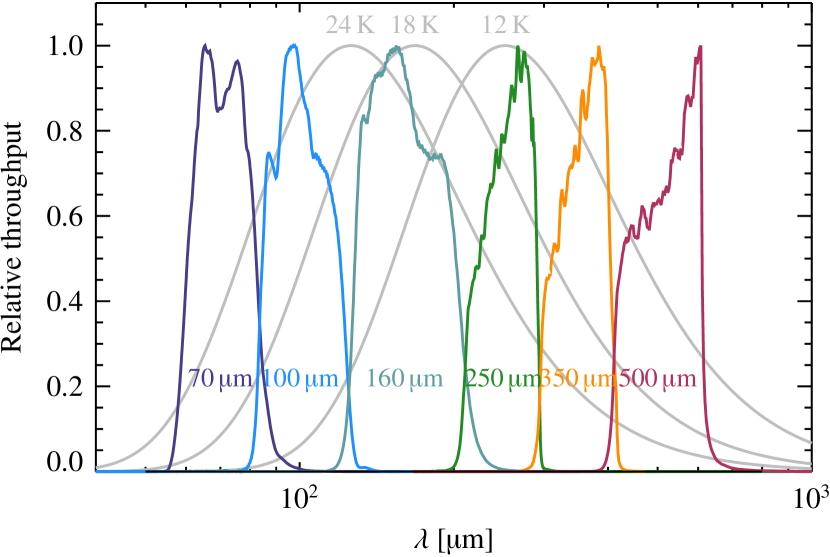
Figure 1: Total throughputs of the PACS and SPIRE bands for extended emission and, superimposed as gray graphs, three modified blackbodies with $T\in\{$12\text{\,}\mathrm{K}$,$18\text{\,}\mathrm{K}$,$24\text{\,}\mathrm{K}$\}$ and with $\beta=1.8$. All lines are in arbitrary units (i.e., the vertical axis only shows relative values).

If we know the optical depth $\tau_{850}$, the effective dust temperature $T$, and the exponent $\beta$ in a given direction of the sky, we can use Eqs. (1–3) to infer the intensity $I_{\nu}$ at each frequency $\nu$. In reality, and if we aim to exploit the higher resolution of Herschel, we only have at our disposal the fluxes measured by the PACS and SPIRE instruments at specific wide bands. For our purposes, it is useful to consider the PACS $100\text{\,}\mathrm{\SIUnitSymbolMicro m}160\text{\,}\mathrm{\SIUnitSymbolMicro m}$ bands, and the SPIRE $250\text{\,}\mathrm{\SIUnitSymbolMicro m}350\text{\,}\mathrm{\SIUnitSymbolMicro m}500\text{\,}\mathrm{\SIUnitSymbolMicro m}$ (the PACS $70\text{\,}\mathrm{\SIUnitSymbolMicro m}$ band is not always optically thin, and in many regions has a very low flux because it is far away from the peak of the blackbody at the temperatures that characterize molecular clouds, $\sim$15\text{\,}\mathrm{K}$$, see Fig. 1).

To solve the inverse problem, that is, infer the optical depth and effective dust temperature (and, eventually, the exponent $\beta$) from the data, we proceeded as follows: we first convolved all Herschel data to the poorest resolution, that is, to $\mathit{FWHM}_{$500\text{\,}\mathrm{\SIUnitSymbolMicro m}$}=$36\text{\,}\mathrm{a}\mathrm{r}\mathrm{c}\mathrm{s}\mathrm{e}\mathrm{c}$$, corresponding to the SPIRE $500\text{\,}\mathrm{\SIUnitSymbolMicro m}$ data; then we performed a fit of the observed spectral energy distribution (SED) by integrating the modified blackbody intensity of Eq. (1) within each Herschel bandpass. For the latter step we used the relative spectral response functions (i.e., the total instrument throughputs) available for the PACS and SPIRE bands, and for SPIRE, as recommended in the SPIRE user manual, we corrected with the $\lambda^{2}$ factor corresponding to the throughput for extended emission, which is appropriate for diffuse emission (higher than the resolution of the instrument).

Figure 2: Composite three-color image showing the Herschel/SPIRE intensities for the region considered, where available (with the $250\text{\,}\mathrm{\SIUnitSymbolMicro m}$, $350\text{\,}\mathrm{\SIUnitSymbolMicro m}$, and $500\text{\,}\mathrm{\SIUnitSymbolMicro m}$ bands shown in blue, green, and red). For regions outside the Herschel coverage, we used the Planck/IRAS dust model $(\tau_{850},T,\beta)$ to predict the intensity that would be observed at the SPIRE passbands. Note that the transition from Herschel to Planck is only visible because of the different resolution, and that otherwise there is no obvious discontinuity in the intensities. user /Subtype /Link /Border [0 0 0]/A ¡¡ /S/JavaScript /JS ( var aOCGs = this.getOCGs(), Layer; var Layers = ”fig:2b,fig:2a”.split(”,”), Active = -1, i, l; for (l=0; l¡Layers.length; l++) Layer = Layers[l]; for (i=0; aOCGs & i¡aOCGs.length; i++) if (aOCGs[i].state aOCGs[i].name == Layer) Active = l; aOCGs[i].state = false; if (Active ¿= 0) break; if (Active == -1) for (l=0; l¡Layers.length; l++) if (Layers[l] == ””) Active = l; Active = Active + 1; if (Active == Layers.length) Active = 0; Layer = Layers[Active]; for (i=0; aOCGs & i¡aOCGs.length; i++) if (aOCGs[i].name == Layer) aOCGs[i].state = true; ) ¿¿ Toggle labels

The Herschel bolometers measure the flux integrated within each filter,

$$\bar{S}=\frac{\int S_{\mathrm{p,e}}(\nu)R_{\mathrm{p,e}}(\nu)\,\mathrm{d}\nu}{\int R_{\mathrm{p,e}}(\nu)\,\mathrm{d}\nu}\,,$$ (4)

where $S_{\mathrm{p,e}}(\nu)$ is the in-beam source flux density and $R_{\mathrm{p,e}}(\nu)$ is the specific passband throughput for point (p) or extended (e) sources (cf. Fig. 1, where $R_{\mathrm{e}}(\nu)$ is reported for the PACS and SPIRE passbands). The Herschel pipeline assumes that the source is point-like and has an SED such that $S_{\mathrm{p}}(\nu)\nu=\mbox{constant}$ across the passband,

$$S_{\mathrm{p}}(\nu)=S_{\mathrm{p}}(\nu_{0})\frac{\nu_{0}}{\nu}\;.$$ (5)

Therefore, the flux provided by the pipeline for each passband corresponds to the flux that a point source with the spectral energy distribution (5) would have at the reference frequency $\nu_{0}$, that is, $S_{\mathrm{p}}(\nu_{0})$. To obtain this quantity, the pipeline converts the measured flux $\bar{S}$ into $S_{\mathrm{p}}(\nu_{0})$ by inserting Eq. (5) into Eq. (4). This yields

$$S_{\mathrm{p}}(\nu_{0})=\left[\frac{\int R_{\mathrm{p}}(\nu)\,\mathrm{d}\nu}{\int(\nu_{0}/\nu)R_{\mathrm{p}}(\nu)\,\mathrm{d}\nu}\right]\bar{S}\equiv K_{\mathrm{4p}}\bar{S}\;,$$ (6)

where, following the notation of the SPIRE observer manual, we have called the correcting factor $K_{\mathrm{4p}}$. In reality, the sources of interest (dark clouds) present extended emission that follows a modified blackbody SED. If we consider the analogous definition of $K_{\mathrm{4e}}$, that is,

$$K_{\mathrm{4e}}\equiv\frac{\int R_{\mathrm{e}}(\nu)\,\mathrm{d}\nu}{\int(\nu_{0}/\nu)R_{\mathrm{e}}(\nu)\,\mathrm{d}\nu}\;,$$ (7)

we can write

$$S_{\mathrm{e}}(\nu_{0})=K_{\mathrm{4e}}\bar{S}=\frac{K_{\mathrm{4e}}}{K_{\mathrm{4p}}}S_{\mathrm{p}}(\nu_{0})=\frac{\int S_{\mathrm{e}}(\nu)R_{\mathrm{e}}(\nu)\,\mathrm{d}\nu}{\int(\nu_{0}/\nu)R_{\mathrm{e}}(\nu)\,\mathrm{d}\nu}\;,$$ (8)

where for the last step we have used Eq. (4).

In summary, Eq. (8) provides a simple way to perform an SED fit on the reduced Herschel data:

• we first multiply for each SPIRE passband the flux reported by the pipeline, that is, $S_{\mathrm{p}}(\nu_{0})$, by the correcting factor $C\equiv K_{\mathrm{4e}}/K_{\mathrm{4p}}=(0.9828,0.9834,0.9710)$ for the $(250,350,500)\,$\mathrm{\SIUnitSymbolMicro m}$$ bands, respectively,

• we then perform an absolute flux calibration for the Herschel bands (see below Sect. 3.3),

• we assume a specific SED, compute the expected extended flux $S_{\mathrm{e}}(\nu_{0})$ at each reference passband $\nu_{0}$ using the r.h.s. of Eq. (8), and

• finally, we modify the SED until we obtain a good match between the observed and theoretical fluxes. For this step we use a simple $\chi^{2}$ minimization that takes into account the calibration errors (that we conservatively take to be equal to $15\%$ in all bands). Because of the degeneracies present in the $\chi^{2}$ minimization, we have kept $\beta$ fixed in the minimization, and fit only $\tau_{850}$ and $T$ to the data. However, the spectral index $\beta$ was not kept constant across a cloud, but instead we used the local value of $\beta$ as estimated from the Planck collaboration (see below Sect. 3.3).

3.3 Absolute fluxes

Since the Herschel SPIRE and PACS bolometers only provide relative photometry, we can only measure gradients of intensities over the observed field. This is usually no problem for point source photometry, but represents a major difficulty for obtaining photometry for extended emission. Before performing the SED fit described in the previous section, therefore, we performed an absolute calibration of all Herschel passbands.

For this purpose, we used the maps released by the Planck collaboration (Planck Collaboration et al., 2011a, b, 2013b). These maps report the results of an all-sky SED fit for a modified blackbody [see Eq. (1)] using the Planck/HFI ($350\text{\,}\mathrm{\SIUnitSymbolMicro m}$ to $2\text{\,}\mathrm{m}\mathrm{m}$) and IRAS ($100\text{\,}\mathrm{\SIUnitSymbolMicro m}$) data. The maps have an intrinsic resolution of $5\text{\,}\mathrm{a}\mathrm{r}\mathrm{c}\mathrm{m}\mathrm{i}\mathrm{n}$ for the optical-depth and effective-dust temperature, and $35\text{\,}\mathrm{a}\mathrm{r}\mathrm{c}\mathrm{m}\mathrm{i}\mathrm{n}$ for the spectral index $\beta$. [Note that the map of the spectral index was also used to derive the local value of $\beta$ that was used in the SED fit described in Sect. 3.2.]

To obtain the absolute flux of each individual Herschel field, we proceeded as follows: from the Planck optical-depth, temperature, and spectral-index map we computed the fluxes expected to be observed by Herschel at the various passbands. For this step, we used the modified black-body model (1), integrated over each passband as in Eq. (8). We then cross-correlated the Herschel observations, degraded to the $5\text{\,}\mathrm{a}\mathrm{r}\mathrm{c}\mathrm{m}\mathrm{i}\mathrm{n}$ resolution, with the computed expected fluxes, and fitted a straight line to the fluxes,

$$S_{\mathrm{e}}(\nu)_{\mathrm{Herschel}}=a_{\nu}+b_{\nu}\,S(\nu)_{\mathrm{Planck}}\;.$$ (9)

The offset $a$ of the linear fit provides the absolute photometric calibration of Herschel. The slopes $b_{\nu}$ are always very close to unity for all frequencies and all regions, which ensures that our methodology is robust and that the Herschel data have a good relative photometry. We repeated the same procedure for each field and each passband separately.

Figure 2 presents a color-composite image of the combined reduced Herschel/SPIRE data for the region considered here, together with the predicted fluxes from Planck at the three SPIRE passbands. This figure graphically depicts the outcome of the procedure described in this section, except that no convolution to the Planck resolution has been performed for the Herschel data (instead, the three SPIRE bands displayed in the figure have been convolved to the $500\text{\,}\mathrm{\SIUnitSymbolMicro m}$ resolution, $36\text{\,}\mathrm{a}\mathrm{r}\mathrm{c}\mathrm{s}\mathrm{e}\mathrm{c}$). From this figure we can also appreciate the temperature differences present in the clouds, which result in different colors across the clouds. Note also that the high-temperature areas, which appear blue in the figure, are generally associated with much brighter emission, a well-known effect of the Planck law (2). Moreover, the colors of the high-resolution regions, observed by Herschel, match the colors of the rest of the field very well, where we used Planck data: this is an additional indication that the absolute calibration of the Herschel fluxes has been successful.

3.4 Extinction conversion

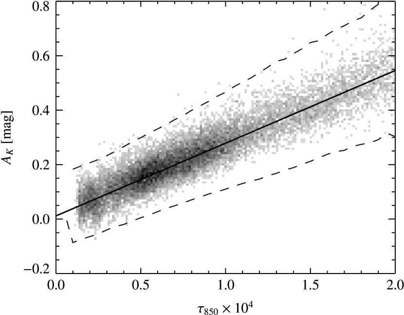
Figure 3: Relationship between submillimiter optical-depth and NIR extinction in Orion A. The best linear fit, used to calibrate the data, is shown together with the expected 3-$\sigma$ region, as calculated from direct error propagation in the extinction map.

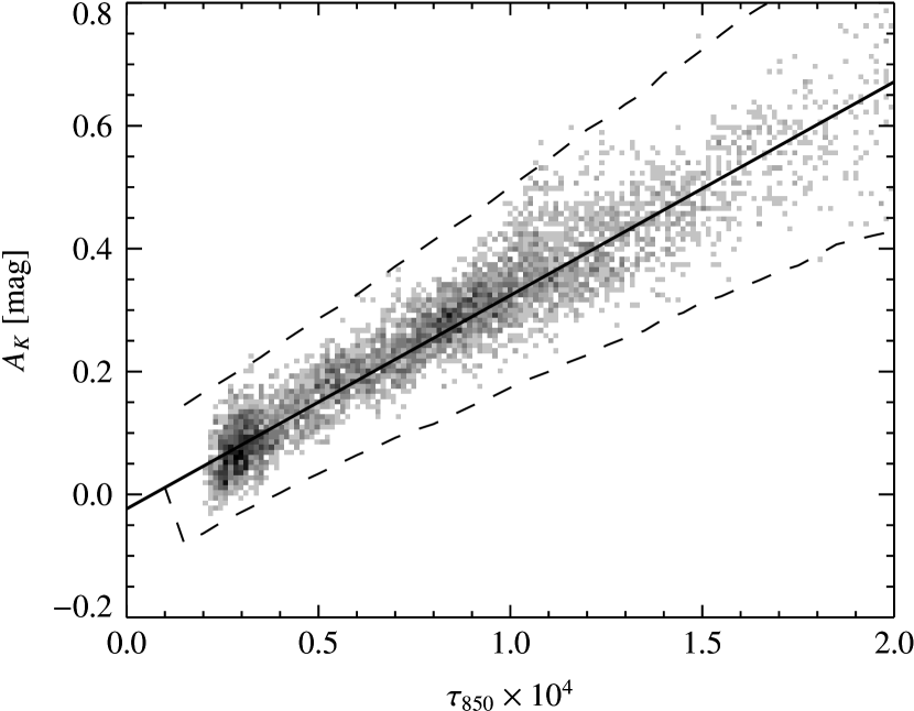
Figure 4: Same as Fig. 3 for Orion B.

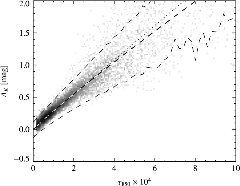
Figure 5: Same as Fig. 3, but for a wider range of values. The plot shows hints of non-linearity for high values of dust column densities or optical-depths, as shown by the curved fit (dashed line). We also report in this plot the linear fit obtained in the range of Fig. 3 (dotted line). A direct comparison between the results obtained from user /Subtype /Link /Border [0 0 0]/A ¡¡ /S/JavaScript /JS ( var aOCGs = this.getOCGs(), Layer; var Layers = ”fig:5a,fig:5b”.split(”,”), Active = -1, i, l; for (l=0; l¡Layers.length; l++) Layer = Layers[l]; for (i=0; aOCGs & i¡aOCGs.length; i++) if (aOCGs[i].state aOCGs[i].name == Layer) Active = l; aOCGs[i].state = false; if (Active ¿= 0) break; if (Active == -1) for (l=0; l¡Layers.length; l++) if (Layers[l] == ””) Active = l; Active = Active + 1; if (Active == Layers.length) Active = 0; Layer = Layers[Active]; for (i=0; aOCGs & i¡aOCGs.length; i++) if (aOCGs[i].name == Layer) aOCGs[i].state = true; ) ¿¿ Nicest and Nicer shows how important it is to account for unresolved substructures and foreground stars in molecular clouds.

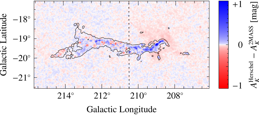
Figure 6: Difference between the extinction predicted by Herschel, using Eq. (11), and the extinction measured with 2MASS/Nicest, with blue (red) indicating a positive (negative) difference. The same figure for Nicer is available on a user /Subtype /Link /Border [0 0 0]/A ¡¡ /S/JavaScript /JS ( var aOCGs = this.getOCGs(), Layer; var Layers = ”fig:6a,fig:6b”.split(”,”), Active = -1, i, l; for (l=0; l¡Layers.length; l++) Layer = Layers[l]; for (i=0; aOCGs & i¡aOCGs.length; i++) if (aOCGs[i].state aOCGs[i].name == Layer) Active = l; aOCGs[i].state = false; if (Active ¿= 0) break; if (Active == -1) for (l=0; l¡Layers.length; l++) if (Layers[l] == ””) Active = l; Active = Active + 1; if (Active == Layers.length) Active = 0; Layer = Layers[Active]; for (i=0; aOCGs & i¡aOCGs.length; i++) if (aOCGs[i].name == Layer) aOCGs[i].state = true; ) ¿¿ different layer.

In principle, one could derive the slope of the linear relationship between the optical-depth $\tau_{850}$ and the dust column by using a suitable model of the interstellar grains:

$$\tau_{\nu}=\kappa_{\nu}\Sigma_{\mathrm{dust}}\;,$$ (10)

where $\kappa_{\nu}$ is the opacity at the frequency $\nu$ and $\Sigma_{\mathrm{dust}}$ is the dust-column density. Determining the dust opacity is a complicated task that requires a detailed knowledge of the dust composition and properties (Ossenkopf & Henning, 1994), which are often highly uncertain. Since we have the NIR extinction map at our disposal, we therefore preferred to derive the dust column-density from $\tau_{850}$ by fitting a linear relationship between $\tau_{850}$ and the $K$-band extinction $A_{K}$, obtained using the Nicest/2MASS technique (Lombardi & Alves, 2001; Lombardi, 2009; Lombardi et al., 2011), after convolving all data to the same resolution (that is, the resolution of the Nicest maps, $\mathit{FWHM}=$3\text{\,}\mathrm{a}\mathrm{r}\mathrm{c}\mathrm{m}\mathrm{i}\mathrm{n}$$):

$$A_{K}=\gamma\tau_{850}+\delta\;.$$ (11)

Note that the slope $\gamma$ is proportional to the ratio of $\kappa_{\mathrm{850}}$, the opacity at $850\text{\,}\mathrm{\SIUnitSymbolMicro m}$, and of $C_{2.2}$, the extinction coefficient at $2.2\text{\,}\mathrm{\SIUnitSymbolMicro m}$, since

$$A_{K}=-2.5\log_{10}\left(\frac{I_{\mathrm{obs}}}{I_{\mathrm{true}}}\right)=(2.5\log_{10}\mathrm{e})\,C_{2.2}\Sigma_{\mathrm{dust}}\;.$$ (12)

Therefore we simply have $\gamma\simeq 1.0857C_{2.2}/\kappa_{850}$. Conversely, we associate the coefficient $\delta$ to either calibration inaccuracies (due, for example, to a control field used in an extinction map that is not completely free of extinction, or to an inaccurate photometric absolute calibration of the Herschel data), or to the presence of dust in the background of the stars used to build the extinction map (that dust would clearly escape extinction measurements, but would still be detected in emission). We found that a single fit within each cloud is satisfactory, but different clouds require different fits. In Figs. 3 and 4 we reports the result of these fits for Orion A and B, limiting the fit only to regions with $\tau_{850}<$2\text{\times}{10}^{-4}$$, where we empirically verified that Eq. (11) is valid. The same figures also report the predicted 3-$\sigma$ boundaries around the fit of Eq. (11), as estimated from the statistical error on the extinction map alone (that is, we ignored errors in the optical-depth). The fact that the datapoints are observed to lie within the marked region proves that fit is very accurate and that the optical-depth map has a negligible error at the resolution of the extinction map (that is, $3\text{\,}\mathrm{a}\mathrm{r}\mathrm{c}\mathrm{m}\mathrm{i}\mathrm{n}$).

In our specific case, we find $\delta_{\mathrm{Orion\ A}}=$0.012\text{\,}\mathrm{m}\mathrm{a}\mathrm{g}$$ and $\delta_{\mathrm{Orion\ B}}=$-0.001\text{\,}\mathrm{m}\mathrm{a}\mathrm{g}$$, while $\gamma_{\mathrm{Orion\ A}}=$2640\text{\,}\mathrm{m}\mathrm{a}\mathrm{g}$$ and $\gamma_{\mathrm{Orion\ B}}=$3460\text{\,}\mathrm{m}\mathrm{a}\mathrm{g}$$. It is leassuring that we measure very low values for both offsets $\delta$; moreover, we do not observe significant differences in the values of $\delta$ and $\gamma$ within the tiles of a single molecular cloud, which would be expected in case of calibration errors (we recall that the absolute flux calibration was performed on each tile individually). This can be regarded as a success both of the calibrations for the extinction maps (through a sensible choice for the control field as operated in Lombardi et al., 2011) and for the Herschel data (through the use of the Planck data).

As mentioned above, the coefficient $\gamma$ is simply linked to the ratio of opacity at $850\text{\,}\mathrm{\SIUnitSymbolMicro m}$ and of extinction at $2.2\text{\,}\mathrm{\SIUnitSymbolMicro m}$ (i.e., the sum of the opacity and scattering coefficient at $2.2\text{\,}\mathrm{\SIUnitSymbolMicro m}$). Differences in the values of $\gamma$, such as those observed here, are probably to be related to differences in the dust composition. Differences in the opacity ratios are indeed common for many similar studies carried out in the past: for example, Kramer et al. (2003) found that the opacity ratios determined toward four cores of the IC 5146 span the range $(1.9\pm 0.2)\text{\times}{10}^{-4}$ to $(5.4\pm 0.3)\text{\times}{10}^{-4}$, which in terms of $\gamma$ would correspond to the range $2000$–$5700$ (see also Shirley et al., 2011). Using the data in Table 1 of Mathis (1990), we can estimate the expected value of $\gamma$. If we take $\beta\simeq 1.8$ (value close to what was measured by Planck in the region we considered), we find

$$\gamma\simeq 1.0857\frac{C_{2.2}}{\kappa_{850}}=\frac{C_{2.2}}{\kappa_{250}}\left(\frac{$850\text{\,}\mathrm{\SIUnitSymbolMicro m}$}{$250\text{\,}\mathrm{\SIUnitSymbolMicro m}$}\right)^{-\beta}\simeq 2\,500\,,$$ (13)

which is very close to our measurements in Orion A and not too far from the value we obtain in Orion B. To reinforce this argument, we also note that a recent analysis of the Planck dust-emission all-sky map (Planck Collaboration et al., 2013a) shows that the dust optical-depth $\tau_{850}$ correlates well with the color excess of quasars, with a relation $E(B-V)=$(1.49\pm 0.03)\text{\times}{10}^{4}$\tau_{850}$, which would imply $\gamma\simeq$4600$$ for $R\equiv A_{V}/E(B-V)=3.1$ and $A_{K}/A_{V}=0.112$ (Rieke & Lebofsky, 1985). However, as noted in Planck Collaboration et al. (2013a), the submillimiter dust opacity can increase by a factor 3 in high-density regions, which would cause $\gamma$ to decrease by a similar factor. In summary, the results for $\gamma$ are perfectly within the currently accepted range of expected values. Instead, our finding seems to be in conflict with the emission and absorption coefficients computed by Weingartner & Draine (2001), which would predict (for their size distribution “B” with $R=5.5$) $\gamma\simeq$4800$$ (and even higher values for lower values of $R$). Since $\gamma$ is directly connected to the grain composition and size distribution, the discrepancy we find might indicate that the Weingartner & Draine (2001) models may need to be revised, at least to explain the dust properties in Orion A and B.

To better understand this problem, we also considered the Ossenkopf & Henning (1994) models. These models provide dust opacities under various conditions, but unfortunately not dust scattering cross-sections. Since extinction is the sum of opacity and scattering, we cannot apply these models directly. To obtain some estimates, however, we assumed the albedo, that is, the ratio between opacity and extinction cross-sections, to be $0.5$ at $2.2\text{\,}\mathrm{\SIUnitSymbolMicro m}$, and 1 at $850\text{\,}\mathrm{\SIUnitSymbolMicro m}$ (in other words, we assumed that opacity has the same cross section of scattering at $2.2\text{\,}\mathrm{\SIUnitSymbolMicro m}$, and that scattering is negligible at $850\text{\,}\mathrm{\SIUnitSymbolMicro m}$). These values, although somewhat arbitrary, agree with the Weingartner & Draine (2001) models. In our conditions, it seems appropriate to use a Mathis et al. (1977) dust distribution with thin ice mantles. Then, for a coagulation time of $1\text{\times}{10}^{5}\text{\,}\mathrm{y}\mathrm{e}\mathrm{a}\mathrm{r}\mathrm{s}$ and a density of $1\text{\times}{10}^{6}\text{\,}\mathrm{c}\mathrm{m}^{-3}$ we find $\gamma\simeq$5100$$ (the predicted value of $\gamma$ decreases to $3700$ for models with a density of $1\text{\times}{10}^{8}\text{\,}\mathrm{c}\mathrm{m}^{-3}$, but this value of course seems inappropriate for giant molecular complexes).

The newer Ormel et al. (2011) models seem instead to be able to reproduce the observed values for $\gamma$. These authors provided a list of opacities and extinction coefficients for a few aggregate models at various coagulation times. For our clouds, it seems reasonable to use coagulation times on the order of 1 to $3\text{\,}\mathrm{M}\mathrm{y}\mathrm{r}$. With this choice, we find very reasonable values for $\gamma$: for example, for the fully ice-coated aggregate (ic-sil, ic-gra) (referred to as “Type-II” mixing in Ormel et al., 2011, and consisting of silicates and graphite grains with ice manthles mixed within the aggregates) the predicted value for $\gamma$ is $\sim$2580$$, very close to our observations for Orion A. On the other hand, if we instead consider the ic-sil+gra model (i.e., a spatial mixture of aggregates consisting of either ice-coated silicate or graphite materials, referred to as “Type-I” mixing), we find $\gamma\simeq$3800$$, not too far from what was observed in Orion B. In summary, although the dust models depends on quite a few parameters (dust composition, mixture type, presence of ice mantles, grain size distribution, coagulation time), we find it possible to accomodate the observed values of gammas within the range of reasonable models.

Across a wider range of opacities (typically, for $\tau_{850}>$2\text{\times}{10}^{-4}$$) the relationship between NIR extinction and optical-depth is no longer linear. A good fit is obtained with the empirical relation

$$A_{K}=c_{1}+c_{2}\tau_{850}^{c_{3}}\;.$$ (14)

Interestingly, for Orion A we are able to recover an almost perfect linearity if we remove the region around the Trapezium from the analysis, that is, for $l>$210.5\text{\,}\mathrm{\SIUnitSymbolDegree}$$ (see Fig. 5). This suggests that the non-linearity is a consequence of including regions for which the 2MASS/Nicest extinctions or the Herschel gray-body SED fit are inaccurate (or both). To better understand this problem, we produced a map that shows the differences between the extinction, as inferred from the optical-depth $\tau_{850}$ used in Eq. (11), and the 2MASS/Nicest extinction (Fig. 6). Note that the blue regions, that is, those where the Herschel column-density exceeds the 2MASS extinction, are mostly confined to the region around the Trapezium and closely follow the locations of known embedded clusters in the cloud. This suggests that the extinction map in these regions is biased low as a result of the contamination from embedded stars (observed therefore through a lower column-density than genuine background stars; see Lombardi, 2009 and Lombardi, 2005 for deeper discussions of these matters). We therefore conclude that the extinction provided by Herschel is more reliable in these regions. The same map also shows an extended light-red area around the ONC. This area correlates very well with the hot regions in Fig. 9, and therefore we suspect that there the Herschel column-density is underestimated. As a likely explanation, we mention temperature gradients along the line of sight (which are probable in regions characterized by a temperature much higher than average), which would induce an underestimate of $\tau_{850}$ (see Sect. 3.1). Interestingly, when Nicer is used, we see that the blue regions tend to fill the entire cloud, indicating that the Nicer extinction map is biased low in all regions with high extinction.

We stress that the test just performed is a strong confirmation of the reliability of extinction studies in regions that are not contaminated by embedded clusters and contain sufficient background stars. Our analysis shows in particular that the extinction measured by Nicest is fully consistent with the completely independent analysis carried out using the Herschel data. Note, however, that a technique such as Nicer, which is optimized but does not take into account the effect of foreground stars or small-scale inhomogeneities, is clearly biased and cannot be used to probe high-column density regions. As discussed in Lombardi (2009), this kind of bias is expected in basically all extinction techniques (with the mentioned exception of Nicest), but this is the first time we are in the position of proving its existence in real data.

Given the results of this section, in the following use only the coefficient $\gamma$ in the conversion from optical-depth to extinction, that is, we set $A_{K}=\gamma\tau_{850}$. Doing so, we ignore $\delta$ because we consider the small measured offsets of Eq. (11) as biases present in the extinction measurements.

3.5 Higher resolution optical-depth maps

We have already mentioned the non-trivial interpretation of the effective dust-temperature. A posteriori, however, one can verify that the derived maps of effective-dust temperature in most cases appear to be significantly smoother than the optical-depth maps (see also below). This observation suggests that we can compute the term $B_{\nu}(T)$ of Eq. (1) using a low-resolution map, and evaluate simply as $\tau_{\nu}=I_{\nu}/B_{\nu}(T)$.

In practice, we applied this technique by using the temperature maps obtained from the modified blackbody fit of the Herschel bands (and therefore computed at the lower resolution, corresponding to $\mathit{FWHM}_{$500\text{\,}\mathrm{\SIUnitSymbolMicro m}$}\simeq$36\text{\,}\mathrm{a}\mathrm{r}\mathrm{c}\mathrm{s}\mathrm{e}\mathrm{c}$$) together with the SPIRE250 intensity maps, which are characterized by $\mathit{FWHM}_{$250\text{\,}\mathrm{\SIUnitSymbolMicro m}$}\simeq$18\text{\,}\mathrm{a}\mathrm{r}\mathrm{c}\mathrm{s}\mathrm{e}\mathrm{c}$$. Hence, this technique allowed us to improve the resolution of our optical-depth maps by a factor two. Note that this technique is the simplest one to derive higher resolution maps from dust-emission data at different resolutions (Juvela et al., 2013). Other options are available (see Juvela & Montillaud, 2013), but the gain obtained is limited, and this is obtained at the price of a significantly more complicated implementation (in particular, the most promising technique, “method E” of Juvela & Montillaud, 2013 cannot be easily used over large regions).

In a sense, the use of a temperature map at the $36\text{\,}\mathrm{a}\mathrm{r}\mathrm{c}\mathrm{s}\mathrm{e}\mathrm{c}$ resolution in an optical-depth SED fit at $18\text{\,}\mathrm{a}\mathrm{r}\mathrm{c}\mathrm{s}\mathrm{e}\mathrm{c}$ is similar to the use of the Planck-fitted spectral index $\beta$ in the SED fit at $36\text{\,}\mathrm{a}\mathrm{r}\mathrm{c}\mathrm{s}\mathrm{e}\mathrm{c}$ resolution. It is nevertheless important to verify the effects of this choice in the final high-resolution optical-depth map. Toward this goal we evaluated the relative variation of the term $B_{\nu}(T)$ for the passband $250\text{\,}\mathrm{\SIUnitSymbolMicro m}$, that is, the multiplicative term in the SED that is temperature dependent, and we verified that it is on the order of $\sim 30\%$. In contrast, the relative change in optical-depth is approximately a factor 10 larger. Hence, the changes in the observed flux at $250\text{\,}\mathrm{\SIUnitSymbolMicro m}$ are clearly dominated by optical-depth gradients and not by temperature gradients, and this justifies the implementation and use of higher resolution maps.

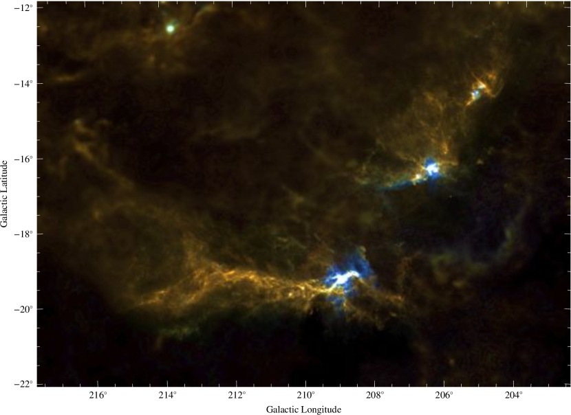
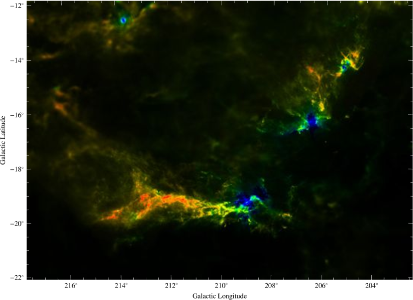
Figure 7: Combined optical depth-temperature map for Orion A and B. The image shows the optical-depth as intensity and the temperature as hue, with red (blue) corresponding to low temperatures (high temperatures). By comparing this image with the one shown in user /Subtype /Link /Border [0 0 0]/A ¡¡ /S/JavaScript /JS ( var aOCGs = this.getOCGs(), Layer; var Layers = ”fig:7b,fig:7a”.split(”,”), Active = -1, i, l; for (l=0; l¡Layers.length; l++) Layer = Layers[l]; for (i=0; aOCGs & i¡aOCGs.length; i++) if (aOCGs[i].state aOCGs[i].name == Layer) Active = l; aOCGs[i].state = false; if (Active ¿= 0) break; if (Active == -1) for (l=0; l¡Layers.length; l++) if (Layers[l] == ””) Active = l; Active = Active + 1; if (Active == Layers.length) Active = 0; Layer = Layers[Active]; for (i=0; aOCGs & i¡aOCGs.length; i++) if (aOCGs[i].name == Layer) aOCGs[i].state = true; ) ¿¿ Figure 1 one can appreciate that regions with relatively high temperatures emit much higher fluxes even if the optical-depth is substantially lower. user /Subtype /Link /Border [0 0 0]/A ¡¡ /S/JavaScript /JS ( var aOCGs = this.getOCGs(), Layer; var Layers = ”fig:7d,fig:7c”.split(”,”), Active = -1, i, l; for (l=0; l¡Layers.length; l++) Layer = Layers[l]; for (i=0; aOCGs & i¡aOCGs.length; i++) if (aOCGs[i].state aOCGs[i].name == Layer) Active = l; aOCGs[i].state = false; if (Active ¿= 0) break; if (Active == -1) for (l=0; l¡Layers.length; l++) if (Layers[l] == ””) Active = l; Active = Active + 1; if (Active == Layers.length) Active = 0; Layer = Layers[Active]; for (i=0; aOCGs & i¡aOCGs.length; i++) if (aOCGs[i].name == Layer) aOCGs[i].state = true; ) ¿¿ Toggle labels

 

Figure 8: Optical-depth map for the field and, on a user /Subtype /Link /Border [0 0 0]/A ¡¡ /S/JavaScript /JS ( var aOCGs = this.getOCGs(), Layer; var Layers = ”fig:8a,fig:8b”.split(”,”), Active = -1, i, l; for (l=0; l¡Layers.length; l++) Layer = Layers[l]; for (i=0; aOCGs & i¡aOCGs.length; i++) if (aOCGs[i].state aOCGs[i].name == Layer) Active = l; aOCGs[i].state = false; if (Active ¿= 0) break; if (Active == -1) for (l=0; l¡Layers.length; l++) if (Layers[l] == ””) Active = l; Active = Active + 1; if (Active == Layers.length) Active = 0; Layer = Layers[Active]; for (i=0; aOCGs & i¡aOCGs.length; i++) if (aOCGs[i].name == Layer) aOCGs[i].state = true; ) ¿¿ different layer, the corresponding error map. The error-map image clearly shows the areas where the Herschel data are available. The resolution of the image varies from $5\text{\,}\mathrm{a}\mathrm{r}\mathrm{c}\mathrm{m}\mathrm{i}\mathrm{n}$ (corresponding to the Planck data) to $36\text{\,}\mathrm{a}\mathrm{r}\mathrm{c}\mathrm{s}\mathrm{e}\mathrm{c}$ (for the Herschel-covered areas).

 

Figure 9: Effective dust-temperature map for the field and, on a user /Subtype /Link /Border [0 0 0]/A ¡¡ /S/JavaScript /JS ( var aOCGs = this.getOCGs(), Layer; var Layers = ”fig:9a,fig:9b”.split(”,”), Active = -1, i, l; for (l=0; l¡Layers.length; l++) Layer = Layers[l]; for (i=0; aOCGs & i¡aOCGs.length; i++) if (aOCGs[i].state aOCGs[i].name == Layer) Active = l; aOCGs[i].state = false; if (Active ¿= 0) break; if (Active == -1) for (l=0; l¡Layers.length; l++) if (Layers[l] == ””) Active = l; Active = Active + 1; if (Active == Layers.length) Active = 0; Layer = Layers[Active]; for (i=0; aOCGs & i¡aOCGs.length; i++) if (aOCGs[i].name == Layer) aOCGs[i].state = true; ) ¿¿ different layer, the corresponding error map. Similarly to Fig. 8, the error-map image shows the areas where the Herschel data are available and the resolution varies from $5\text{\,}\mathrm{a}\mathrm{r}\mathrm{c}\mathrm{m}\mathrm{i}\mathrm{n}$ (corresponding to the Planck data) to $36\text{\,}\mathrm{a}\mathrm{r}\mathrm{c}\mathrm{s}\mathrm{e}\mathrm{c}$ (for the Herschel-covered areas).

3.6 Implementation

A specific C code was written to perform various steps of the pipeline, and in particular the SED fit. The code is fully parallel and takes advantages of the linear dependences of the models on parameters [for example, the linear dependence of the modified blackbody model (1) on the optical-depth $\tau_{850}$]; all this allowed us to analyze large regions very quickly. The nonlinear chi-square minimization was performed using the C-version of the MINPACK-1 least squares fitting library.

In a typical pipeline run we perform the following steps:

1. We perform a standard reduction of Herschel data and multiply the SPIRE data by the $C$ correcting factors. At the same time, we produce an extinction map in the same area using data from the 2MASS-PSC archive, and also retrieve the optical-depth, temperature, and spectral-index maps created by the Planck collaboration.

2. We convolve the Herschel reduced images to reach a $5\text{\,}\mathrm{a}\mathrm{r}\mathrm{c}\mathrm{m}\mathrm{i}\mathrm{n}$ resolution, and we warp and re-grid the images to match the Planck data projection.

3. We generate from the Planck data the expected fluxes at Herschel passbands, and we compare this pixel by pixel. By performing the linear fit of Eq. (9) we recover the offset $a$ of each Herschel waveband and verify that the linear coefficient $b$ is close to unity.

4. We return to the reduced Herschel images (whose fluxes are now absolutely calibrated) and convolve them to the same resolution (typically, the $36\text{\,}\mathrm{a}\mathrm{r}\mathrm{c}\mathrm{s}\mathrm{e}\mathrm{c}$ resolution of the SPIRE $500\text{\,}\mathrm{\SIUnitSymbolMicro m}$ data).

5. We perform an SED fit pixel by pixel using a modified blackbody as a model, leaving the optical-depth and effective-dust temperature as free parameters; in contrast, the local value of the spectral index $\beta$ is taken from the Planck/IRAS fit.

6. Finally, we also build a higher resolution map from the SPIRE $250\text{\,}\mathrm{\SIUnitSymbolMicro m}$ band by inferring the optical-depth from the observed flux (and assuming the $\beta$ from the Planck and $T$ from the $36\text{\,}\mathrm{a}\mathrm{r}\mathrm{c}\mathrm{s}\mathrm{e}\mathrm{c}$ resolution SED fit).

4 Results

4.1 Optical-depth and temperature maps

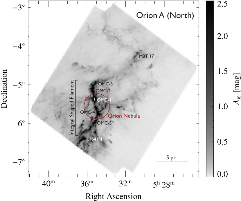
Figure 10: Optical-depth map of Orion A central at a resolution of $18\text{\,}\mathrm{a}\mathrm{r}\mathrm{c}\mathrm{s}\mathrm{e}\mathrm{c}$, converted into units of $A_{K}$ from cross-correlation with the 2MASS/Nicest map.

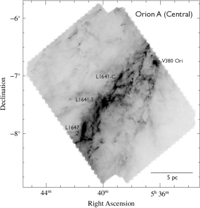
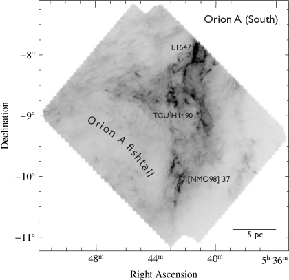
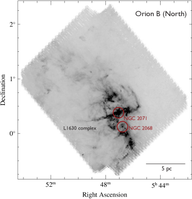
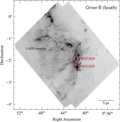
Figure 11: Same as Fig. 10 for Orion A north, Orion A south, Orion B north, and Orion B NN.

The main final products of our custom pipeline are the optical-depth and temperature maps of the region. To exploit the unique sensitivity and the large-scale view of the entire molecular cloud complex provided by Planck, we combined the Herschel map with the Planck/IRAS data, even though there is a large difference in resolution between these data ($36\text{\,}\mathrm{a}\mathrm{r}\mathrm{c}\mathrm{s}\mathrm{e}\mathrm{c}$ vs. $5\text{\,}\mathrm{a}\mathrm{r}\mathrm{c}\mathrm{m}\mathrm{i}\mathrm{n}$).

Figure 7 shows the combined optical-depth-temperature map: the effective dust temperature is represented using different values of hue (from red for $T\leq$12\text{\,}\mathrm{K}$$ to blue for $T\geq$30\text{\,}\mathrm{K}$$), while the intensity is proportional to the optical depth. This representation has the advantage of showing all the main final products in a single image and of suppressing the relatively large uncertainties on the effective dust temperature present in the Herschel tiles when the amount of dust, and thus the optical-depth, are low. It is also interesting to compare Fig. 7 with Fig. 2 and directly appreciate how relatively hot regions in the maps, typically associated with hot early-type stars, are in Fig. 2.

Figure 8 individually shows the optical-depth measured in the whole field by either Herschel or Planck/IRAS. On a different layer, the figure also reports the associated errors, which are typically around $5\text{\times}{10}^{-6}$ for the Herschel data. The Planck data have significantly smaller errors (mostly because of the much longer exposure time), but of course have a much poorer resolution. The error map is also useful to visually reveal the exact shapes of the areas covered by Herschel.

The corresponding effective-dust temperature map is shown in Fig. 9, together with its error (on a different layer). It is interesting to observe a number of features of this image. First, the specific area considered shows a relatively wide range of temperatures, in particularly related to OB stars present in the massive star-forming regions (the Orion Nebula Cluster, NGC 2024 in Orion B, and the Mon R2 cluster). It is also evident that the temperature drops in dense regions of the cloud (provided there are no early-type stars present in the region): this is particularly evident in the “spine” of the Orion A molecular cloud.

The error on the temperature map has a wide range as well. The largest error on the temperature is observed within the Herschel boundaries, but outside the densest regions of the cloud (in particular, to the west of Orion A, where it reaches values of $3\text{\,}\mathrm{K}4\text{\,}\mathrm{K}$). Instead, errors on the effective dust temperature in regions where the optical-depth is high can be as low as $\sim$0.1\text{\,}\mathrm{K}$$, similar to lower than the errors observed in the Planck region. Regions at the boundaries of the Herschel coverage and with large errors on the effective dust temperature are often associated with mismatches with the Planck data. These systematic mismatches are due to a combination of the low signal-to-noise ratio and of the different wavelength coverage of the maps.

Finally, we note that the Planck temperature maps show clear ringing around bright areas. These artifacts are a result of the use of different wavelengths (with slightly different resolutions) in nonlinear algorithms in the Planck pipeline.

Figures 10 and 11 show the optical-depth maps of several regions of Orion A and B at the $18\text{\,}\mathrm{a}\mathrm{r}\mathrm{c}\mathrm{s}\mathrm{e}\mathrm{c}$ resolution. These maps have been obtained using the technique described in Sect. 3.5 (we prefer to show individual regions in separate figures to better show the level of detail achieved). Note that for these higher resolution maps we do not report any error estimate, since assessing the error is non-trivial. We can isolate three main sources of errors, however: the statistical, photometric error on the SPIRE250 flux (which directly propagates to an error in the final optical-depth); the statistical error on the temperature (which propagates to the optical-depth through the Planck function $B_{\nu}(T)$ at $\lambda=$250\text{\,}\mathrm{\SIUnitSymbolMicro m}$$, and which is also correlated to the error on the SPIRE250 flux); and the error on the temperature due to the different resolution (which of course is not statistical in nature and thus difficult to quantify).

4.2 Validation

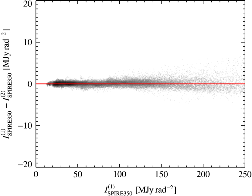
Figure 12: Relationship between the SPIRE 350 fluxes as measured on Orion A southern and central fields (which are partially overlapping), after absolute flux calibration. The median of the flux difference between the two fields, $\sim$56\text{\,}\mathrm{k}\mathrm{J}\mathrm{y}\,\mathrm{r}\mathrm{a}\mathrm{d}^{-2}$$ is approximately 6 times lower than the average noise level, and more than 1 000 times lower than the median flux level in the overlapping area.

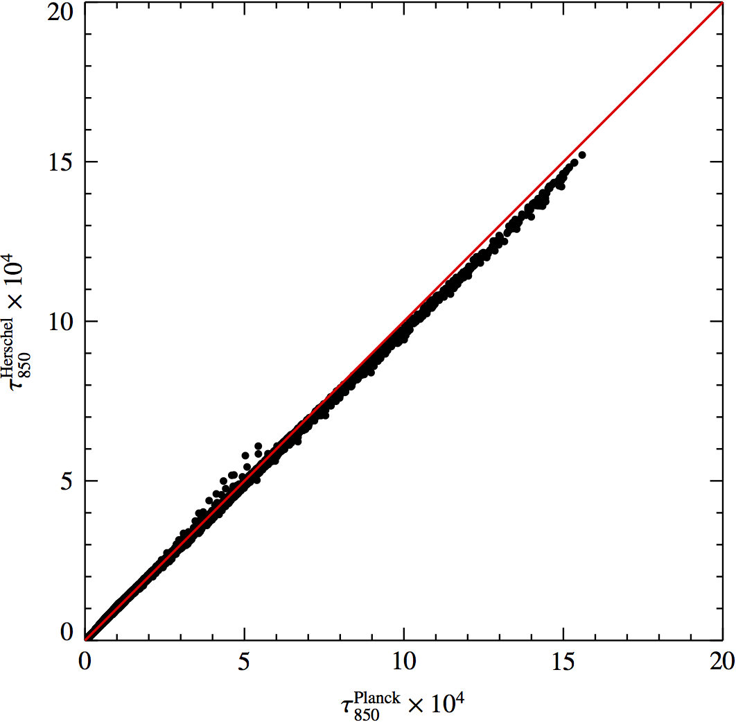
Figure 13: Comparison between the optical-depth derived from the Planck data and that derived from our calibration of the Herschel data in Orion A, after convolving them at the resolution of Planck ($5\text{\,}\mathrm{a}\mathrm{r}\mathrm{c}\mathrm{m}\mathrm{i}\mathrm{n}$). The excellent agreement confirms that the Herschel data are perfectly calibrated to Planck and that the derived optical-depth does not show any systematic effect.

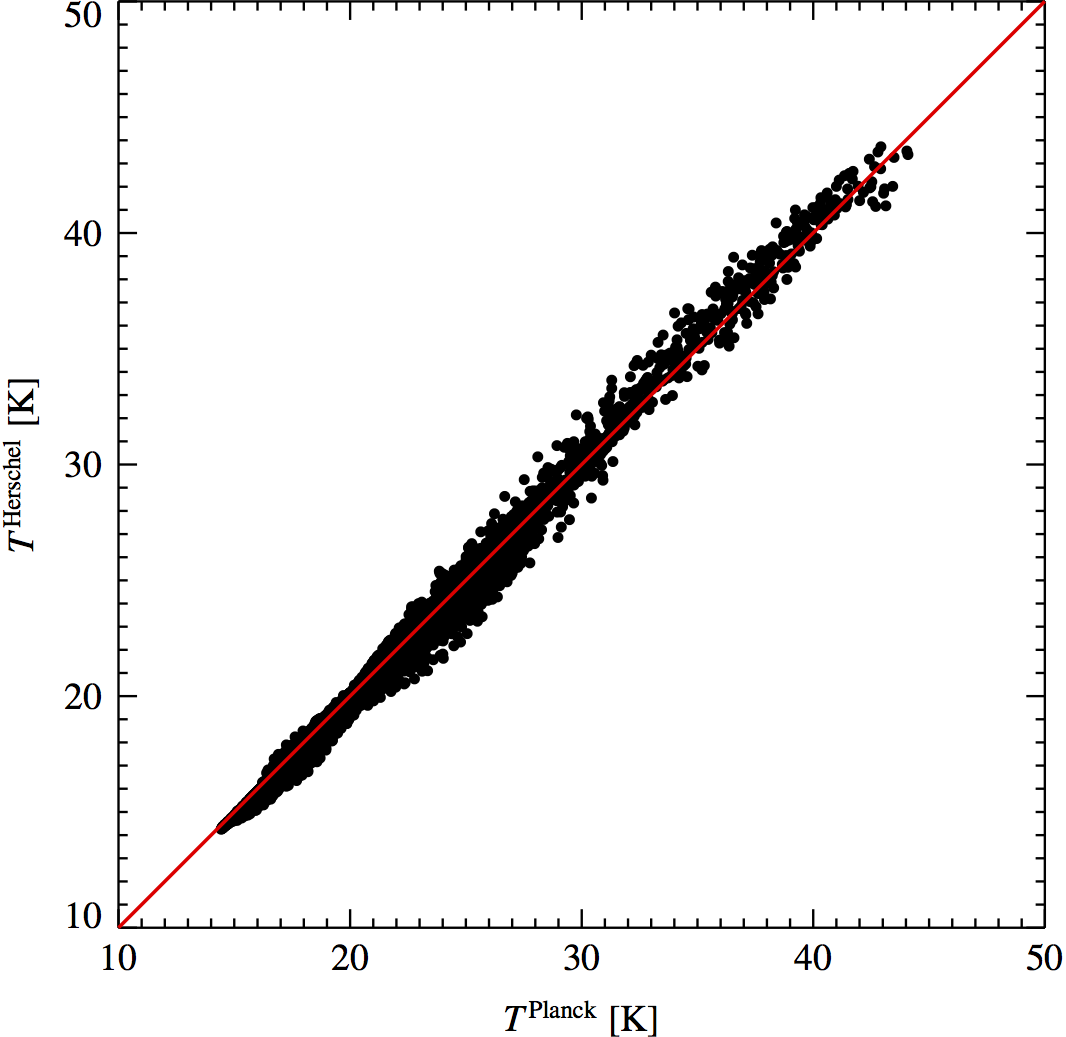
Figure 14: Comparison between the effective dust temperature derived from the Planck data and that derived from our calibration of the Herschel data in Orion B, after convolving them at the resolution of Planck ($5\text{\,}\mathrm{a}\mathrm{r}\mathrm{c}\mathrm{m}\mathrm{i}\mathrm{n}$).

It is obvious that in general the results obtained appear to be reliable: the shapes of the clouds are the ones we know from independent measurements, the ranges of effective dust temperatures measured are reasonable, and the fact that the effective dust temperature drops in the dense regions is consistent with our expectations. However, we clearly need to and can go beyond these simple qualitative aspects to assess the reliability of our data. Indeed, throughout the analysis we have performed a series of tests to cross-validate the results. In this section, we intend to summarize these tests (some of which were mentioned in Sect. 3) and to present new ones.

One of the critical aspects of calibrating Herschel data is the removal of the offsets in the individual bands and fields, in other words, the conversion from relative to absolute fluxes. As explained, this is achieved by direct comparison with the predicted fluxes from the optical-depth, temperature, and spectral index from the Planck maps. We can check this step in two different ways during the calibration: (1) as mentioned above, the calibration slope, that is, parameter $b$ of Eq. (9), must be close to unity and (2) in overlapping areas of independent Herschel observations, the fluxes measured must agree. We performed both checks, and the results of one of the second tests, the comparison of the SPIRE 250 fluxes in the Orion south and central fields, are reported in Fig. 12.

Figures 3 and 14 provide another indirect check of the consistency of the data. These plots show the relationship between the submillimiter optical-depth and the extinction, or equivalently, the ratio of extinction at $2.2\text{\,}\mathrm{\SIUnitSymbolMicro m}$ and opacity at $850\text{\,}\mathrm{\SIUnitSymbolMicro m}$, $C_{2.2}/\kappa_{850}$ in the range $\tau_{850}<$2\text{\times}{10}^{-4}$$. Since both the submillimeter optical-depth and the extinction are directly proportional to the dust column-density, we expect to see a linear relation, and indeed this is what we observe (up to high extinctions, provided Nicest is used). Additionally, the scatter observed around the linear fit is fully consistent with the error in the extinction measurements (which, we recall, are based on relatively shallow 2MASS data).

A similar check can be carried out by comparing the optical depth as derived from the Herschel data with that obtained by the Planck team. To carry out this test we first convolved all Herschel bands to $5\text{\,}\mathrm{a}\mathrm{r}\mathrm{c}\mathrm{m}\mathrm{i}\mathrm{n}$ resolution and then performed an SED fit on the convolved data. The results of this process are shown in Figs. 13 and 14. It is interesting to note that the perfect agreement observed in Fig. 13 does not hold if we reverse the steps, that is, if we first perform an SED fit at the Herschel resolution, and then convolve the optical-depth map obtain to the $5\text{\,}\mathrm{a}\mathrm{r}\mathrm{c}\mathrm{m}\mathrm{i}\mathrm{n}$ resolution of Planck: this is because the overall fit involves highly nonlinear equations.

5 Discussion

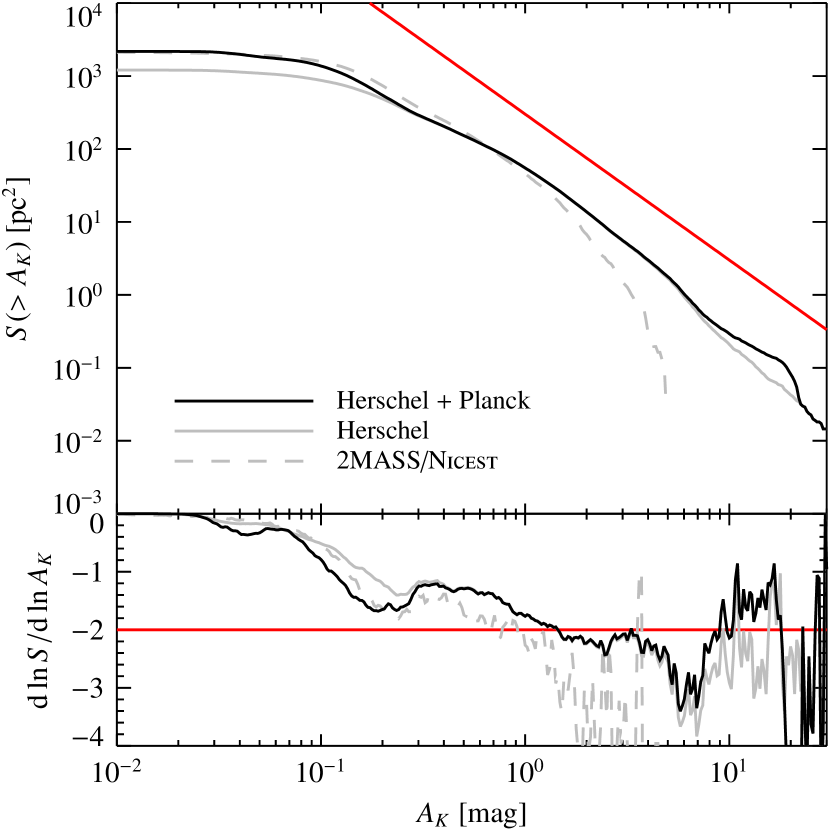
Figure 15: Integral area-extinction relation for Orion A, i.e., the physical cloud area above a given extinction threshold (top panel), and the logarithmic derivative of this quantity (bottom panel). The solid black line shows the result for the entire field, while the solid gray line shows the region covered by Herschel alone. For comparison we also plot as a dashed gray line the same quantity as obtained from the 2MASS/Nicest extinction map and a simple $S(>A_{K})\propto A_{K}^{-2}$ relation as a red line.

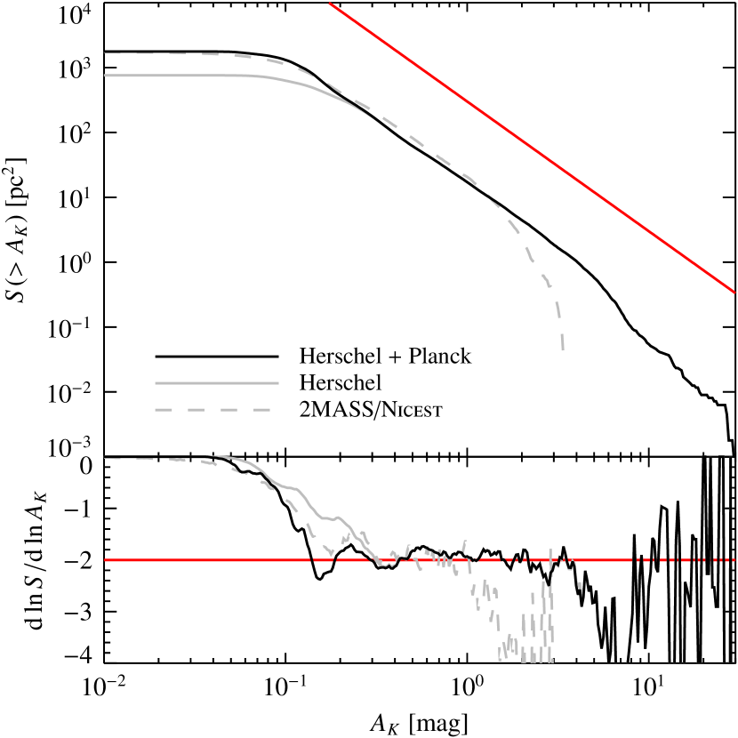
Figure 16: Same as Fig. 15 for Orion B.

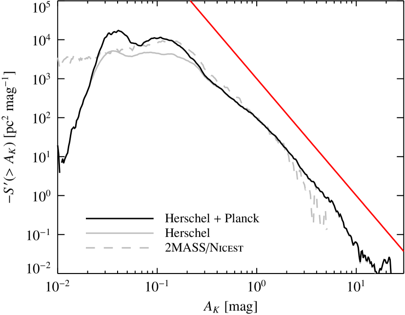
Figure 17: Function $-S^{\prime}(>A_{K})$, that is, the probability distribution function (pdf) of the measured column densities for Orion A. In this log-log plot a log-normal distribution would appear as a parabola, and a power law as a straight line. The red line shows the slope of the power law $-S^{\prime}(A_{K})\propto A_{K}^{-3}$.

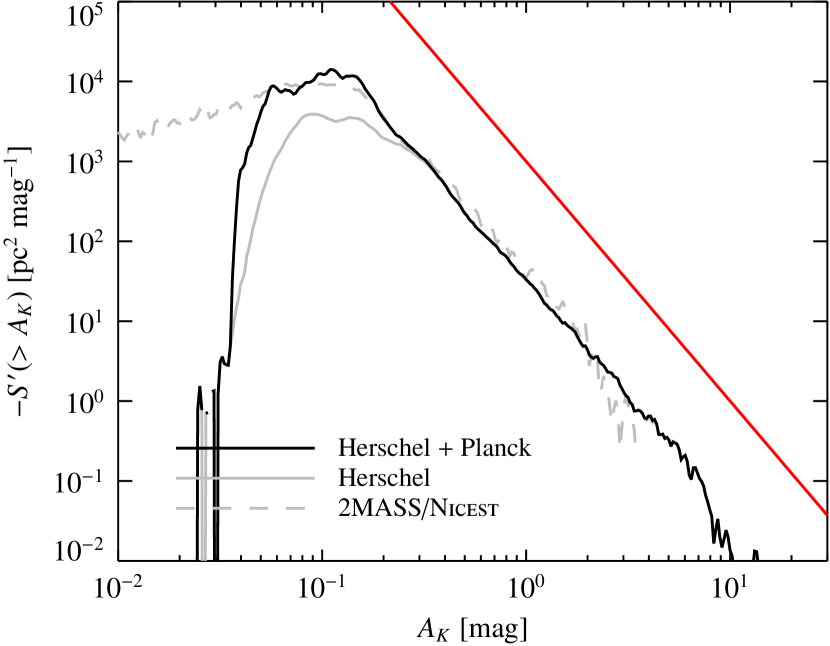
Figure 18: Same as Fig. 17 for Orion B.

The maps we presented can be used for many different purposes, and it is certainly beyond the scope of this paper to explore all of them in detail. Here we just present a few immediate applications, leaving the rest to follow-up papers.

Figures 15 and 16 show the integral area functions $S(>A_{K})$, that is, the cloud area, measured in square parsecs, above the extinction threshold $A_{K}$, as a function of $A_{K}$. The two figures refer to Orion A and B, and for both clouds we assumed a distance of $414\text{\,}\mathrm{p}\mathrm{c}$ (Menten et al., 2007). We defined the boundaries of the clouds to be

Orion A: $$206 {}\leq l\leq 217\;, -21\leq b\leq-17\;,$$

Orion B: $$203 {}\leq l\leq 210\;, -17\leq b\leq-12\;.$$ (15)

Furthermore, we plot the area functions obtained only in the Herschel covered area (gray solid line), in the total region that identifies each cloud (black solid line), and as obtained from the Nicest/2MASS data (gray dashed line). Note that the gray solid line is below the black one for low column densities, a result of the limited area covered by the Herschel survey. At the other extreme, for high column densities, the dashed line is consistently below the solid ones, a result of the poorer resolution and smaller dynamic range of the extinction map derived from the relatively shallow 2MASS data. The solid lines are generally identical in the region covered by the Herschel survey (that is, for $A_{K}\gtrsim$0.1\text{\,}\mathrm{m}\mathrm{a}\mathrm{g}$$), except for a small “bump” of the black line in Orion A for $A_{K}\sim$10\text{\,}\mathrm{m}\mathrm{a}\mathrm{g}$$, because of the lack of Herschel data at the center of the OMC due to saturation (see Fig. 10, white area to the left of the “OMC-1” label). Note also that the lowest value for $S(>A_{K})$ plotted in Figs. 15 and 16, $1\text{\times}{10}^{-2}\text{\,}\mathrm{p}\mathrm{c}^{2}$, corresponds to $\sim$8\text{\,}\mathrm{p}\mathrm{i}\mathrm{x}\mathrm{e}\mathrm{l}$$ in the $36\text{\,}\mathrm{a}\mathrm{r}\mathrm{c}\mathrm{s}\mathrm{e}\mathrm{c}$ resolution optical-depth maps.

For Orion A, and even more for Orion B, the $S$ function in a wide range follows an $A_{K}^{-2}$ slope, indicated by the red line. As a possible explanation of this result, we consider a simple toy model. The gas in molecular clouds is approximately isothermal, a result of the combined heating of the gas from cosmic rays and cooling from CO (Goldsmith & Langer, 1978). Therefore, in our toy model it does not seem unreasonable to use a radial profile $\rho(r)\propto 1/r^{2}$ for the dense regions of molecular clouds, corresponding to the singular isothermal sphere solution (a non-singular isothermal profiles would follow the $1/r^{2}$ slope at radii larger than the core). In projection, such a density profile would produce a surface density profile $\Sigma_{\mathrm{gas}}(r)\propto A_{K}(r)\propto 1/r$. Hence, the cloud area above a given extinction threshold in this simple model would follow the relation $S(>A_{K})\propto r^{2}\propto A_{K}^{-2}$. Note that this simple argument applies to the gas component and not to the dust component (which, instead, is easily heated by starlight). However, since the gas constitutes the large majority of mass in the cloud, it is this component that sets the shape of the $S(>A_{K})$ relation; the dust here is merely used as a tracer.

The bottom plots of Figs. 15 and 16 show the logarithmic derivative of $S(>A_{K})$. Figure 16 shows that the Orion B cloud is very well described by the $S(>A_{K})\propto A_{K}^{-2}$ scaling law over nearly two orders of magnitude in extinction, from $A_{K}\sim 0.1$ to $5\text{\,}\mathrm{m}\mathrm{a}\mathrm{g}$. The $S$ function for Orion A (Fig. 15) is not as well described by a single power-law index, but over the same extinction range its slope is quite close to -2, being somewhat shallower below $A_{K}\sim$1.0\text{\,}\mathrm{m}\mathrm{a}\mathrm{g}$$ and somewhat steeper above $A_{K}\sim$1.0\text{\,}\mathrm{m}\mathrm{a}\mathrm{g}$$. At lower column densities, we observe a clear break of the relation, with the cumulative area function $S(>A_{K})$ approximately constant. This is likely due to the limited area considered in making Figs. 15 and 16; however, it is obvious that this scaling law cannot hold at arbitrarily lower column densities for at least two reasons: first, one inevitably would be outside the survey area when $A_{K}$ becomes very small; second, physically it is not plausible that regions with a very low column-density remain isothermal. From this latter point of view, it is intriguing to note that the break at low extinctions is observed around $A_{K}\sim$0.1\text{\,}\mathrm{m}\mathrm{a}\mathrm{g}$$, a value where most likely the dust shielding just starts to become effective enough to isolate the gas in the inner part of the molecular clouds from the interstellar radiation field, thus enabling isothermal density distributions above this threshold. Interestingly, this is approximately the same column-density as for the survival of ¹²CO. At the other extreme, the scaling law seems to break for column densities just below $10\text{\,}\mathrm{m}\mathrm{a}\mathrm{g}$. We note, however, that it is not obvious that this break is real, as it might be a result of systematic effects that are possibly present at high column densities. We mention as a probable source of biases temperature gradients along the line of sight, which are thus completely unaccounted for in the SED fit.

Figures 17 and 18 show the differential area function, or more precisely, $-S^{\prime}(>A_{K})$. This function is just proportional to the probability distribution function of column-densities (pdf), a function often considered in the context of molecular cloud studies. It is generally accepted that this function has a log-normal shape as a result of the turbulent supersonic motion that are believed to characterize molecular clouds on large scales (e.g. Vazquez-Semadeni, 1994; Padoan et al., 1997; Passot & Vázquez-Semadeni, 1998; Scalo et al., 1998). However, as shown by Tassis et al. (2010), log-normal distributions are also expected under completely different physical conditions (also plausible for molecular clouds), such as radially stratified density distributions dominated by gravity and thermal pressure, or by a gravitationally driven ambipolar diffusion. Vice versa, the log-normality of the pdf has been challenged in clouds located in isolated environments such as Corona (Alves et al., 2014). Surprisingly, our study suggests that the log-normal regime, if at all present in the cloud studied here, is confined to very low column densities, below $A_{K}\sim$0.1\text{\,}\mathrm{m}\mathrm{a}\mathrm{g}$$; for higher column densities we again find the scaling-law relation $S^{\prime}(>A_{K})\propto A_{K}^{-3}$. Although this behavior has been observed in the past, especially in star-forming clouds (Kainulainen et al., 2009), we are now in the position to demonstrate that the power-law regime dominates most ranges of column-densities and generally characterizes the cloud structure above $A_{K}\sim$0.1\text{\,}\mathrm{m}\mathrm{a}\mathrm{g}$$. We also stress that this limit, corresponding to $1\text{\,}\mathrm{m}\mathrm{a}\mathrm{g}$ of visual extinction, really marks the boundary of molecular clouds and is, for instance, also associated to the limit for the photodissociation of carbon monoxide.

Figures 19 and 20 show the integral mass functions $M(>A_{K})$, that is, the cloud mass above the extinction threshold $A_{K}$, as a function of $A_{K}$. As before, we plot mass functions corresponding to the various dataset using different line colors and styles. The mass was estimated by converting the column-density into a surface mass density using the factor

$$\frac{\Sigma}{A_{K}}=\mu\beta_{K}m_{\mathrm{p}}\simeq$183\text{\,}\mathrm{M}_{$\odot$}\,\mathrm{p}\mathrm{c}^{-2}$\,,$$ (16)

where $\mu\simeq 1.37$ is the mean molecular weight corrected for the helium abundance, $\beta_{K}\simeq$1.67\text{\times}{10}^{22}\text{\,}\mathrm{c}\mathrm{m}^{-2}\,\mathrm{m}\mathrm{a}\mathrm{g}^{-1}$$ is the gas-to-dust ratio, that is, $[N(\textsc{Hi})+2N(H_{2}))]/A_{K}$ (Savage & Mathis, 1979; Lilley, 1955; Bohlin et al., 1978; see also Rieke & Lebofsky, 1985 for the conversion from $A_{K}$ to $A_{V}$ for 2MASS), and $m_{\mathrm{p}}=$1.67\text{\times}{10}^{-24}\text{\,}\mathrm{g}$$ is the proton mass.

Note the very good agreement of at low column densities between the solid black and dashed gray lines, that is, between the “total” masses measured from Herschel + Planck and from 2MASS/Nicest: this clearly is a result of using 2MASS to calibrate the $\gamma$ factor.

Figure 19: Integral mass-extinction relation for Orion A, i.e. the cloud mass above a given extinction threshold. The color codes follow the same convention as in Fig. 15.

Figure 20: Same as Fig. 19 for Orion B.

Not unexpectedly, both mass functions of Orion A and B approximately follow an $A_{K}^{-1}$ slope. This is a direct consequence of the fact that the area functions follow an $A_{K}^{-2}$ slope, since we have

$$M(>A_{K})\propto\int_{A_{K}}^{\infty}\frac{\mathrm{d}S(>A_{K}^{\prime})}{\mathrm{d}A_{K}^{\prime}}A_{K}^{\prime}\,\mathrm{d}A_{K}^{\prime}\;.$$ (17)

Figure 21: Posterior probability distributions for the four parameters of the model described in Eqs. (18) and (19), obtained with a Markov chain Monte Carlo algorithm for Orion A. The obtained best-fit values and their formal errors are $\kappa=$1.18\pm 0.09\text{\,}\mathrm{s}\mathrm{t}\mathrm{a}\mathrm{r}\mathrm{s}\,\mathrm{p}\mathrm{c}^{-2}\,\mathrm{m}\mathrm{a}\mathrm{g}^{-\beta}$$, $\beta=$1.99\pm 0.05$$, $A_{0}=$0.050\pm 0.028\text{\,}\mathrm{m}\mathrm{a}\mathrm{g}$$, and $\sigma=$0.0088\pm 0.0049\text{\,}\mathrm{p}\mathrm{c}$$.

Figure 22: Fractional number of protostars in Orion A above a given extinction threshold as a function of the threshold, together with a few predictions from simple power-law models. The curve for $\beta=2$ agrees well with the data up to $A_{K}=$6\text{\,}\mathrm{m}\mathrm{a}\mathrm{g}$$.

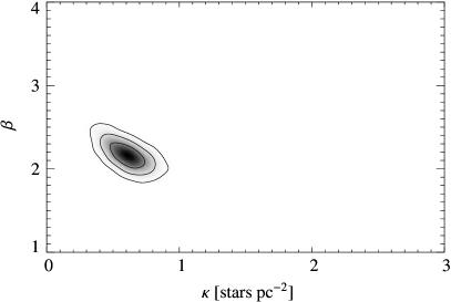
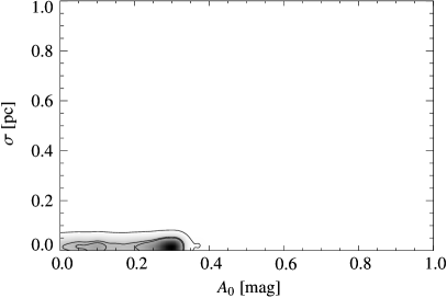
Figure 23: Posterior-probability distributions for the four parameters of the model described in Eqs. (18) and (19), obtained with a Markov chain Monte Carlo algorithm for Orion B. The obtained best-fit values and their formal errors are $\kappa=$0.60\pm 0.10\text{\,}\mathrm{s}\mathrm{t}\mathrm{a}\mathrm{r}\mathrm{s}\,\mathrm{p}\mathrm{c}^{-2}\,\mathrm{m}\mathrm{a}\mathrm{g}^{-\beta}$$, $\beta=$2.16\pm 0.10$$, $A_{0}=$0.20\pm 0.10\text{\,}\mathrm{m}\mathrm{a}\mathrm{g}$$, and $\sigma=$0.018\pm 0.007\text{\,}\mathrm{p}\mathrm{c}$$.

Figure 24: Fractional number of protostars in Orion B above a given extinction threshold as a function of the threshold, together with a few predictions from simple power-law models. The curve for $\beta=2$ agrees well with the data up to $A_{K}=$6\text{\,}\mathrm{m}\mathrm{a}\mathrm{g}$$.

Figure 25: Behavior of the $\beta$ exponent for increasingly coarser resolutions for Orion A and Orion B. The data have been obtained by repeating the parameter inference for the model of Eqs. (18) and (19) on images smoothed with different kernel sizes. The dashed lines show the result of two simple rational fits for data of the form $\beta=(\beta_{0}+a\,\mathit{FWHM})/(1+b\,\mathrm{FWHM})$, which seems to reproduce the data well. The best-fit parameters obtained for the two clouds are $\beta_{0}=$1.82\pm 0.14$$ for Orion A and $\beta_{0}=$1.92\pm 0.24$$ for Orion B.

A possible different application of our maps is to test the validity of the Kennicutt-Schmidt relation (Schmidt, 1959; Kennicutt, 1998). This relation refers to globally averaged surface densities of the star formation rate ($\Sigma_{\mathrm{SFR}}$) and the gas ($\Sigma_{\mathrm{gas}}$) in galaxies. Recently, we investigated the local form of this relation (Lombardi et al., 2013) by modeling star formation events in molecular clouds as a (possibly delayed) Poisson spatial process. We showed that the local protostar surface density is simply proportional to the square of the projected gas density, or equivalently to the square of the column-density, $A_{K}$. In this respect, it is interesting to consider a simple model of star formation where the predicted density of protostars at the position $x$, $\Sigma_{\mathrm{YSO}}(x)$, is written as the convolution of a primordial density of protostars $\Sigma^{(0)}_{\mathrm{YSO}}(x)$ with a Gaussian kernel:

$$\Sigma_{\mathrm{YSO}}(x)=\int\frac{1}{2\pi\sigma^{2}}\mathrm{e}^{|x-x^{\prime}|^{2}/2\sigma^{2}}\Sigma_{\mathrm{YSO}}^{\mathrm{(0)}}(x^{\prime})\,\mathrm{d}^{2}x^{\prime}\;.$$ (18)

The convolution is used to model the fact that the star-formation process is not instantaneous, and during this process the protostars might become displace from the original sites of their formation. Finally, we model the primordial density of protostars as

$$\Sigma_{\mathrm{YSO}}^{\mathrm{(0)}}(x)=\kappa\operatorname{H}\bigl{(}A_{K}(x)-A_{0}\bigr{)}\left(\frac{A_{K}}{1\mbox{ mag}}\right)^{\beta}(x)\;,$$ (19)

where $\operatorname{H}$ is the Heaviside function

$$\operatorname{H}(z)=\begin{cases}1&\text{if $z>0\;,$}\\ 0&\text{if $z\leq 0\;.$}\end{cases}$$ (20)

Therefore, in our model the constants involved are the normalization $\kappa$ (taken to be measured in units of $\mathrm{s}\mathrm{t}\mathrm{a}\mathrm{r}\,\mathrm{p}\mathrm{c}^{-2}\,\mathrm{m}\mathrm{a}\mathrm{g}^{-\beta}$), the star formation threshold $A_{0}$ (in units of $K$-band extinction), the dimensionless exponent $\beta$, and the diffusion coefficient $\sigma$ (measured in $\mathrm{p}\mathrm{c}$).

Using the technique described in Lombardi et al. (2013), we can use a catalog of protostars and a map of the cloud column-density to infer the values of the four parameters of the model. As a sample application, we show here the results obtained for Orion A using the Spitzer-based catalog of protostars of Megeath et al. (2012) (see Lombardi et al., 2013 and Lada et al., 2013 for further details on the specific data used).

The results for Orion A, reported in Figs. 21 and 22, show that the simple relation $\Sigma_{\mathrm{YSO}}\propto A_{K}^{2}$ is confirmed to describe the local star formation process in Orion A well (more precisely, we find $\beta=$1.99\pm 0.05$$ within $1$-$\sigma$; but see the figures for detailed credibility regions). However, Fig. 22 also shows that for $A_{K}>$6\text{\,}\mathrm{m}\mathrm{a}\mathrm{g}$$ the observed number of protostars seems to be below the prediction given by the simple relation $\Sigma_{\mathrm{YSO}}\propto A_{K}^{2}$. Several realistic processes might produce this effect: it might be a genuine result of evolutionary effects (not all the high-density gas might yet have produced stars, or stars might have moved from their sites of formation), or it might be an observational artifact (small-number statistics or simply our inhability to detect all protostars because of confusion effects). Furthermore, the value of $\kappa$ is significantly below than the value measured by Lombardi et al. (2013) using the 2MASS/Nicest map ($1.18\pm 0.09\text{\,}\mathrm{s}\mathrm{t}\mathrm{a}\mathrm{r}\mathrm{s}\,\mathrm{p}\mathrm{c}^{-2}\,\mathrm{m}\mathrm{a}\mathrm{g}^{-\beta}$ vs. $1.64\pm 0.09\text{\,}\mathrm{s}\mathrm{t}\mathrm{a}\mathrm{r}\mathrm{s}\,\mathrm{p}\mathrm{c}^{-2}\,\mathrm{m}\mathrm{a}\mathrm{g}^{-\beta}$). This is to be expected, since $\kappa$ is quite sensitive to changes of resolution: high-resolution maps probe the small peaks of molecular clouds better, where significant star formation occurs. In particular, if $\beta>1$, we expect that a smoothing in the measured map is associated with a higher measured value of $\kappa$, to compensate for the “missed” star-forming density in the high-density peaks. In contrast, the value of $\beta$ appears to be more robust (see discussion below).

The results for Orion B are shown in Figs. 23 and 24. The parameters obtained in this cloud are consistent with those of Orion A; in particular, the simple $\Sigma_{\mathrm{YSO}}\propto A_{K}^{2}$ relation is verified: we measure $\beta=$2.16\pm 0.10$$. The result is somewhat surprising, since in Lada et al. (2013) we found instead that the star formation in Orion B would follow a $\beta\simeq 3$ law. A closer investigation shows that this discrepancy can be essentially attributed to resolution effects. To prove this assertion, we repeated the entire local Schmidt-law analysis using maps with degraded resolution. The results obtained for both Orion A and B are shown in Fig. 25: they show that $\beta$ clearly increases with the final FWHM of the images, the effect being limited for Orion A, and much more substantial for Orion B. Moreover, it appears that the data to the left of the plot converge around $\beta\simeq 2$ for both clouds.

Interestingly, in Orion B we also see a hint for a threshold in the star-forming rate, that is, it seems probable that $A_{0}$ is strictly positive, which is confirming a similar result (Lada et al., 2013). We stress, however, that even the current data cannot exclude the case $A_{0}\simeq$0\text{\,}\mathrm{m}\mathrm{a}\mathrm{g}$$.

In summary, it is intriguing that different clouds seem to be characterized by essentially the same local Schmidt-law and also show the same distribution functions of dense gas, with $S(>A_{K})\propto A_{K}^{2}$. These two facts together might be the key to understanding the good correlation found by Lada et al. (2010) between the mass of dense gas and the star formation rate in local molecular clouds.

6 Conclusions

Our main results can be summarized in the following items:

• We presented optical-depth and temperature maps of the entire Orion molecular cloud complex obtained from Herschel and Planck space observatories.

• The maps have a $36\text{\,}\mathrm{a}\mathrm{r}\mathrm{c}\mathrm{s}\mathrm{e}\mathrm{c}$ resolution for Herschel observations and a $5\text{\,}\mathrm{a}\mathrm{r}\mathrm{c}\mathrm{m}\mathrm{i}\mathrm{n}$ resolution elsewhere. In addition, we also produced a $18\text{\,}\mathrm{a}\mathrm{r}\mathrm{c}\mathrm{s}\mathrm{e}\mathrm{c}$ resolution optical-depth maps based on the SPIRE 250 data alone.

• We calibrated the optical-depth maps using 2MASS/Nicest extinction data, thus obtaining column-density extinction maps at the resolution of Herschel with a dynamic range $1\text{\times}{10}^{-2}\text{\,}\mathrm{m}\mathrm{a}\mathrm{g}$ to $30\text{\,}\mathrm{m}\mathrm{a}\mathrm{g}$ of $A_{K}$, or from $4\text{\times}{10}^{20}\text{\,}\mathrm{c}\mathrm{m}^{-2}$ to $6\text{\times}{10}^{23}\text{\,}\mathrm{c}\mathrm{m}^{-2}$.

• We measured $C_{2.2}/\kappa_{850}$, that is, the ratio of the $2.2\text{\,}\mathrm{\SIUnitSymbolMicro m}$ extinction coefficient and of the $850\text{\,}\mathrm{\SIUnitSymbolMicro m}$ opacity. We found that the values obtained for both Orion A and B cannot be explained using the Ossenkopf & Henning (1994) or the Weingartner & Draine (2001) theoretical models of dust, but agree very well with the newer Ormel et al. (2011) models for ice-covered silicate-graphite conglomerate grains.

• We examined the cumulative and differential area functions of the data, showing that over a large regime of extinction we observe a power-law $S(>A_{K})\propto A_{K}^{-2}$, which is reminiscent of a simple isothermal model of molecular clouds; surprisingly, we do not see clear evidence of log-normality in the column-density pdf.

• We used the Planck/Herschel maps to re-evaluate the local Schmidt-law for star formation, $\Sigma_{YSO}\propto A_{K}^{\beta}$. We found that $\beta\simeq 2$ in Orion A, confirming our earlier studies (Lombardi et al., 2013; Lada et al., 2013). For Orion B, we also found $\beta\simeq 2$, which is lower than our previous estimates as a result of the much improved angular resolution of the Herschel observations.

Appendix A Hidden layers of multiple-layer figures

In this appendix we provide a “flat” version of the hidden layers of multi-layer figures, useful if no JavaScript-enabled PDF reader is used, or for the printed version of the paper.

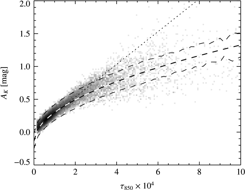
Figure 26: Relationship between submillimiter optical-depth and Nicer extinction map in Orion A. The plot shows clear nonlinear effects for high values of dust column-densities or optical-depths, as shown by the curved fit (dashed line). We also report in this plot the linear fit obtained in the range of Fig. 3 (dotted line). The same figure with Nicest technique is provided in Fig. 5.

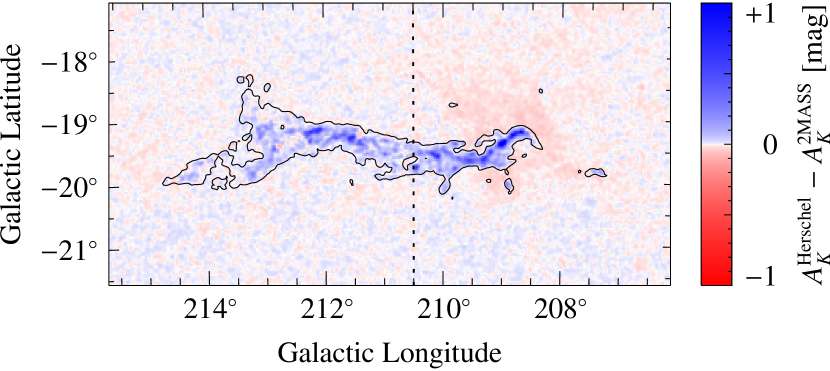
Figure 27: Difference between the extinction predicted by Herschel, using Eq. (11), and the extinction measured with 2MASS/Nicer, with blue (red) indicating a positive (negative) difference. The same plot for Nicest is available in Fig. 6.

Figure 28: Error on the optical-depth for the image reported in Fig. 8. The figure clearly shows the areas where the Herschel data are available. The resolution of the image varies from $5\text{\,}\mathrm{a}\mathrm{r}\mathrm{c}\mathrm{m}\mathrm{i}\mathrm{n}$ (corresponding to the Planck data) to $36\text{\,}\mathrm{a}\mathrm{r}\mathrm{c}\mathrm{s}\mathrm{e}\mathrm{c}$ (for the Herschel-covered areas).

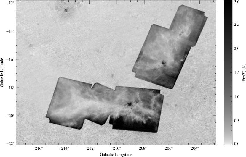
Figure 29: Error on the effective dust temperature for the image reported in Fig. 9.

References

- Alves et al. (1998) Alves, J., Lada, C. J., Lada, E. A., Kenyon, S. J., & Phelps, R. 1998, ApJ, 506, 292
- Alves et al. (2014) Alves, J., Lombardi, M., & Lada, C. 2014, ArXiv 1401.2857A
- André et al. (2010) André, P., Men’shchikov, A., Bontemps, S., et al. 2010, A&A, 518, L102
- Ascenso et al. (2013) Ascenso, J., Lada, C. J., Alves, J., Román-Zúñiga, C. G., & Lombardi, M. 2013, A&A, 549, A135
- Bally (2008) Bally, J. 2008, in Handbook of Star Forming Regions, Volume I, ed. B. Reipurth (Astronomical Society of the Pacific), 459
- Blaauw (1991) Blaauw, A. 1991, in NATO ASIC Proc. 342: The Physics of Star Formation and Early Stellar Evolution, ed. C. J. Lada & N. D. Kylafis, 125
- Bohlin et al. (1978) Bohlin, R. C., Savage, B. D., & Drake, J. F. 1978, ApJ, 224, 132
- Brown et al. (1995) Brown, A. G. A., Hartmann, D., & Burton, W. B. 1995, A&A, 300, 903
- Da Rio et al. (2012) Da Rio, N., Robberto, M., Hillenbrand, L. A., Henning, T., & Stassun, K. G. 2012, ApJ, 748, 14
- Goldsmith & Langer (1978) Goldsmith, P. F. & Langer, W. D. 1978, ApJ, 222, 881
- Goodman et al. (2009) Goodman, A. A., Pineda, J. E., & Schnee, S. L. 2009, ApJ, 692, 91
- Griffin et al. (2010) Griffin, M. J., Abergel, A., Abreu, A., et al. 2010, A&A, 518, L3
- Hillenbrand (1997) Hillenbrand, L. A. 1997, AJ, 113, 1733
- Juvela et al. (2013) Juvela, M., Malinen, J., & Lunttila, T. 2013, A&A, 553, A113
- Juvela & Montillaud (2013) Juvela, M. & Montillaud, J. 2013, A&A, 557, A73
- Kainulainen et al. (2009) Kainulainen, J., Beuther, H., Henning, T., & Plume, R. 2009, A&A, 508, L35
- Kennicutt (1998) Kennicutt, Jr., R. C. 1998, ApJ, 498, 541
- Kramer et al. (2003) Kramer, C., Richer, J., Mookerjea, B., Alves, J., & Lada, C. 2003, A&A, 399, 1073
- Lada et al. (1994) Lada, C. J., Lada, E. A., Clemens, D. P., & Bally, J. 1994, ApJ, 429, 694
- Lada et al. (2010) Lada, C. J., Lombardi, M., & Alves, J. F. 2010, ApJ, 724, 687
- Lada et al. (2013) Lada, C. J., Lombardi, M., Roman-Zuniga, C., Forbrich, J., & Alves, J. F. 2013, ApJ, 778, 133
- Lada et al. (2000) Lada, C. J., Muench, A. A., Haisch, Jr., K. E., et al. 2000, AJ, 120, 3162
- Lamarre et al. (2010) Lamarre, J.-M., Puget, J.-L., Ade, P. A. R., et al. 2010, A&A, 520, A9
- Lilley (1955) Lilley, A. E. 1955, ApJ, 121, 559
- Lombardi (2005) Lombardi, M. 2005, A&A, 438, 169
- Lombardi (2009) Lombardi, M. 2009, A&A, 493, 735
- Lombardi & Alves (2001) Lombardi, M. & Alves, J. 2001, A&A, 377, 1023
- Lombardi et al. (2006) Lombardi, M., Alves, J., & Lada, C. J. 2006, A&A, 454, 781
- Lombardi et al. (2011) Lombardi, M., Alves, J., & Lada, C. J. 2011, A&A, 535, A16
- Lombardi et al. (2008) Lombardi, M., Lada, C. J., & Alves, J. 2008, A&A, 489, 143
- Lombardi et al. (2010) Lombardi, M., Lada, C. J., & Alves, J. 2010, A&A, 512, A67
- Lombardi et al. (2013) Lombardi, M., Lada, C. J., & Alves, J. 2013, A&A, 559, A90
- Maddalena et al. (1986) Maddalena, R. J., Morris, M., Moscowitz, J., & Thaddeus, P. 1986, ApJ, 303, 375
- Malinen et al. (2011) Malinen, J., Juvela, M., Collins, D. C., Lunttila, T., & Padoan, P. 2011, A&A, 530, A101
- Mathis (1990) Mathis, J. S. 1990, ARA&A, 28, 37
- Mathis et al. (1977) Mathis, J. S., Rumpl, W., & Nordsieck, K. H. 1977, ApJ, 217, 425
- Megeath et al. (2012) Megeath, S. T., Gutermuth, R., Muzerolle, J., et al. 2012, AJ, 144, 192
- Menten et al. (2007) Menten, K. M., Reid, M. J., Forbrich, J., & Brunthaler, A. 2007, A&A, 474, 515
- Muench et al. (2008) Muench, A., Getman, K., Hillenbrand, L., & Preibisch, T. 2008, in Handbook of Star Forming Regions, Volume I, ed. B. Reipurth (Astronomical Society of the Pacific), 483
- Muench et al. (2002) Muench, A. A., Lada, E. A., Lada, C. J., & Alves, J. 2002, ApJ, 573, 366
- Ormel et al. (2011) Ormel, C. W., Min, M., Tielens, A. G. G. M., Dominik, C., & Paszun, D. 2011, A&A, 532, A43
- Ossenkopf & Henning (1994) Ossenkopf, V. & Henning, T. 1994, A&A, 291, 943
- Ott (2010) Ott, S. 2010, in Astronomical Society of the Pacific Conference Series, Vol. 434, Astronomical Data Analysis Software and Systems XIX, ed. Y. Mizumoto, K.-I. Morita, & M. Ohishi, 139
- Padoan et al. (1997) Padoan, P., Jones, B. J. T., & Nordlund, A. P. 1997, ApJ, 474, 730
- Passot & Vázquez-Semadeni (1998) Passot, T. & Vázquez-Semadeni, E. 1998, Phys. Rev. E, 58, 4501
- Pilbratt et al. (2010) Pilbratt, G. L., Riedinger, J. R., Passvogel, T., et al. 2010, A&A, 518, L1
- Planck Collaboration et al. (2013a) Planck Collaboration, Abergel, A., Ade, P. A. R., et al. 2013a, ArXiv 1312.1300P
- Planck Collaboration et al. (2013b) Planck Collaboration, Ade, P. A. R., Aghanim, N., et al. 2013b, ArXiv 1303.5062P
- Planck Collaboration et al. (2011a) Planck Collaboration, Ade, P. A. R., Aghanim, N., et al. 2011a, A&A, 536, A1
- Planck Collaboration et al. (2011b) Planck Collaboration, Ade, P. A. R., Aghanim, N., et al. 2011b, A&A, 536, A19
- Planck HFI Core Team et al. (2011) Planck HFI Core Team, Ade, P. A. R., Aghanim, N., et al. 2011, A&A, 536, A6
- Poglitsch et al. (2010) Poglitsch, A., Waelkens, C., Geis, N., et al. 2010, A&A, 518, L2
- Rieke & Lebofsky (1985) Rieke, G. H. & Lebofsky, M. J. 1985, ApJ, 288, 618
- Robberto et al. (2013) Robberto, M., Soderblom, D. R., Bergeron, E., et al. 2013, ApJS, 207, 10
- Roussel (2012) Roussel, H. 2012, Scanamorphos: Maps from scan observations made with bolometer arrays, astrophysics Source Code Library
- Savage & Mathis (1979) Savage, B. D. & Mathis, J. S. 1979, ARA&A, 17, 73
- Scalo et al. (1998) Scalo, J., Vazquez-Semadeni, E., Chappell, D., & Passot, T. 1998, ApJ, 504, 835
- Schmidt (1959) Schmidt, M. 1959, ApJ, 129, 243
- Schneider et al. (2013) Schneider, N., André, P., Könyves, V., et al. 2013, ApJ, 766, L17
- Shetty et al. (2009) Shetty, R., Kauffmann, J., Schnee, S., Goodman, A. A., & Ercolano, B. 2009, ApJ, 696, 2234
- Shirley et al. (2011) Shirley, Y. L., Huard, T. L., Pontoppidan, K. M., et al. 2011, ApJ, 728, 143
- Tassis et al. (2010) Tassis, K., Christie, D. A., Urban, A., et al. 2010, MNRAS, 408, 1089
- Tauber et al. (2010) Tauber, J. A., Mandolesi, N., Puget, J.-L., et al. 2010, A&A, 520, A1
- Vazquez-Semadeni (1994) Vazquez-Semadeni, E. 1994, ApJ, 423, 681
- Weingartner & Draine (2001) Weingartner, J. C. & Draine, B. T. 2001, ApJ, 548, 296
- Wilson et al. (2005) Wilson, B. A., Dame, T. M., Masheder, M. R. W., & Thaddeus, P. 2005, A&A, 430, 523