An efficient GPU acceptance-rejection algorithm for the selection of the next reaction to occur for Stochastic Simulation Algorithms

Abstract

1 Motivation:

The Stochastic Simulation Algorithm (SSA) has largely diffused in the field of systems biology. This approach needs many realizations for establishing statistical results on the system under study. It is very computationnally demanding, and with the advent of large models this burden is increasing. Hence parallel implementation of SSA are needed to address these needs.

At the very heart of the SSA is the selection of the next reaction to occur at each time step, and to the best of our knowledge all implementations are based on an inverse transformation method. However, this method involves a random number of steps to select this next reaction and is poorly amenable to a parallel implementation.

2 Results:

Here, we introduce a parallel acceptance-rejection algorithm to select the K next reactions to occur. This algorithm uses a deterministic number of steps, a property well suited to a parallel implementation. It is simple and small, accurate and scalable. We propose a Graphics Processing Unit (GPU) implementation and validate our algorithm with simulated propensity distributions and the propensity distribution of a large model of yeast iron metabolism. We show that our algorithm can handle thousands of selections of next reaction to occur in parallel on the GPU, paving the way to massive SSA.

3 Availability:

We present our GPU-AR algorithm that focuses on the very heart of the SSA. We do not embed our algorithm within a full implementation in order to stay pedagogical and allows its rapid implementation in existing software. We hope that it will enable stochastic modelers to implement our algorithm with the benefits of their own optimizations.

4 Contact:

mestivier@ijm.univ-paris-diderot.frmestivier@ijm.univ-paris-diderot.fr

5 Introduction

It is now widely acknowledged that stochasticity is an inherent feature of many biological systems, mainly due to the small populations of certain reactants species (McAdams1997 ; Thattai2001 ; Paulsson2004 ). This inherent randomness cannot be dealted with deterministic approaches, and stochastic simulations are required in order to achieve more accurate simulations.

For complex networks, such as encountered in systems biology, each chemical species can be implicated in many interactions with the other components. This results in complex temporal behaviors and computer simulations are an essential tools in order to understand its dynamics (Achcar2011 ; Endy2001 ; Arkin1998 ).

The Stochastic Simulation Algorithm (SSA) was introduced by D.T. Gillespie more than 30 years ago (Gillespie1976 ; Gillespie1977 ), and has now diffuses among different scientific communities, in particular in the field of systems biology. Many implementations have been proposed (see Pahle2008 for a review, LeNovere2001 ; Zhou2011 ; Stoll2012 ) in order to popularize its use among modelers and biologists.

However, stochastic systems need many realizations in order to capture enough statistical information on the system under study, and are thus computationnally demanding. With the advent of large models in systems biology, this burden is still increasing.

As an illustration, a recent model for iron homeostasis in the yeast Saccharomyces cerevisiae incorporates 641 species and 1029 reactions and is simulated using a boolean version of the SSA (Achcar2011 ). Such large models have to be challenged using a huge amount of datasets in order to assess their correctness, at the cost of many simulations. As an example, the sensitivity analysis involves testing 9 different values of the parameter of each of the 1029 reactions, with 1000 realizations (See: Additional File 2 in Achcar2011 ) for computing statistics, hence such a sensitivity analysis needs $9\times 1029\times 1000=9261000$ realizations. Moreover, this model of iron homeostasis was also validated by the confrontation of the output of the simulations mimicking different biological contexts to more than 190 phenotypic mutants, metabolomic data and the global analysis of more than 180 in silico mutants.

In order to tackle this “need for power”, two directions of research have been explored over the last few years: the first accelerates individual simulations starting from the original formulations proposed by Gillespie Gillespie1976 ; Gillespie1977 . The second exploits parallel architectures in order to run multiple realizations of the algorithm.

As will be developped in the Methods section, the system under study is defined by $N$ chemical or biological species and by $M$ chemical reactions that describe their interactions. The SSA characterizes each reaction by a propensity function $\alpha_{j}$ that allows one to compute, at each iteration of the algorithm, the probability that this specific reaction will be the next to occur.

It is well-known that this heart of the SSA is the most computationnally costly part of the algorithm Komarov2012 .

Hence, the acceleration of individual simulation mainly focuses on modifications of this selection of the index $j$ of the next reaction to occur (see Li2008 for a review).

For example, Gibson (Gibson2000 ) introduced the Next Reaction Method (NRM), and a dependency graph which lists the propensity functions that depend on the outcome of each reaction, enabling them to identify and alter only propensity functions which require updating. Cao (Cao2004 ) proposed an Optimized Direct Method (ODM), with a modification of the selection of the next reaction to occur that implies the ordering of propensity functions in a search list so that reactions occuring more frequently are the first in the list. Another proposed acceleration by McCollum et al. (McCollum2006 ) is the Sorting Direct Method (SDM) that dynamically changes the reaction order, which changes the propensity functions order, the more probable being the first. In the same spirit of reducting search depth, Li (Li2006 ) introducted the Logarithmic Direct Method (LDM) which uses a binary search to determine which reaction is due to fire next.

The second direction uses the advent of parallel architectures such as Graphics Processing Units (GPU) in order to perform many realizations of the stochastic algorithm to speed-up the overal runtime (Komarov2012 ; Zhou2011 ; Gillespie2012 ; Li2008 ; Gillespie2013 ; Li2009 ; Tian2005 ; Burrage2006 ; Klingbeil2011 ).

In every parallel implementation, each CPU core or GPU thread runs one realization of the SSA, which means that each GPU thread is considered as an individual unit. Each algorithm can also implement some of the acceleration techniques developped for serial simulation, at the cost of the complexity of the data structure.

Then, it becomes feasible to run hundreds of realizations of the same stochastic model and they allow a scaleup that depends on the size of the system.

However, to the best of our knowledge, the chemical systems considered are often small systems, ranging from few species and reactions to less than one hundred species and reactions. Recent approaches extend these limits (see for example the hybrid approaches of Komarov et al. Komarov2012 that enables larger models).

It is widely accepted that it is extremely difficult to implement efficiently the stochastic algorthim on GPU Klingbeil2011 ; Zhou2011 . And it is then anticipated that such approaches will be limited with the growing number of large models that systems biology generates.

For parallel implementations, the limitation comes from the fact that each thread of the GPU had to manage a realization of a simulation. This means that each thread had to implement a complete algorithm. Because the memory used by each threads on one SM of the GPU is a limited, it is possible to launch many realizations of a stochastic simulations only for small models.

In the literature on stochastic simulation, the selection from the propensity distribution in order to select the next reaction index $j$ is done using an inversion transformation (IT) method. This method uses one uniform random number $u$ and iterate in the cumulative distribution of the (normalized) propensities until it exceed $u$. This choice is justified by the poor performance of classical acceptance-rejection (AR) methods. However, the IT method involves a non-deterministic number of steps. From a parallel point of view, running $K$ realizations in parallel with such an algorithm imposes that some realizations have to wait for the others to finish, hence wasting resources and impeding parallel performances.

Our purpose in this paper is to propose a new direction of research effort by introducting a parallel acceptance-rejection algorithm to select in parallel the $K$ next reactions to occur. This choice comes from the following lines of evidence: At each time step of the SSA, the propensity functions for every reaction can be considered as a discrete distribution (called in this paper the propensity distribution), from which one will select a reaction index $j$. This propensity distribution is updated at each time step, but here, we will focus only on the heart of the SSA, i.e. the selection of the next reaction to occur. This algorithm involves the same number of steps that enables one to run $K$ realizations in parallel without wasting hardware resources.

We show that this algorithm is very simple and that it uses little memory space, which leaves more ressources for the other parts (typically other optimizations) of a stochastic simulation algorithm.

We propose an implementation of a GPU hardware, but our algorithm can be transposed to other parallel architectures. Therefore we want to stay general and pedagogical and we do not embed our GPU/AR algorithm procedure in a complete stochastic algorithm code.

Our GPU/AR algorithm addresses the heart the SSA and we envision that many stochastic modelers would prefer to adapt our algorithm to their optimizations and data structures rather than consider a new implementation that might not fit their needs.

We hope that the simplicity of our GPU-AR algorithm will help stochastic modelers to implement new simulation codes that could address the new challenge of the stochastic simulations of large models.

6 Methods

6.1 Graphics Processing Units

Graphics Processing Units (GPUs) are a set of cores on a graphical card that allow one to off-load multiple instances of the same computations applied to large data sets, referred to as a data-parallel computing model.

The basic execution unit on a GPU is a thread that synchronously executes the same set of instructions, called a kernel, on different cores of a single multiprocessor on different data pieces indexed by the thread ID. Threads are grouped into blocks. These blocks are assigned to run on streaming multiprocessors, each of which is composed of a programmer-defined number of threads.

GPU’s can be seen as massively parallel many-core co-processors that are capable of TFLOPS.

The NVIDIA Corporation introduced the Compute Unified Device Architecture (CUDA) Farber2011 ; Sanders2010 which enables developers to write programs for the NVIDIA GPU using a minimally extended version of the C language.

One important point is that not all algorithms, often developped for sequential architectures, are well-adapted to the GPU massive parallel nature. More importantly, developers should develop new algorithms in order to capture this massive parallel nature. This paper belong to this effort.

6.2 The Stochastic Simulation Algorithm

Briefly, the system is described by $N$ molecular species ${E_{1},\cdots,E_{N}}$, represented by the dynamical state vector $X(t)=(X_{1}(t),\cdots,X_{N}(t))$ where $X_{i}(t)$ is the number of molecules of species $E_{i}$ in the system at time $t$. $M$ chemical reactions ${R_{1},\cdots,R_{M}}$ describe how these $N$ species are in interaction (See (Li2008 ) for a general presentation).

Each reaction $R_{j}$ is characterized by a propensity function $a_{j}$ (with $\alpha_{0}=\sum_{j=1}^{M}\alpha_{j}$) and a change state vector $v_{j}={v_{1j},\cdots,v_{Nj}}$ (the propensity function is updated at each time step of the simulation.)

At a given time step $t$ of the simulation, the propensity value $a_{j}$ allows one to compute the probability, given the state of the system $X(t)$, that the reaction $R_{j}$ will occur in the next time interval $[t,t+\tau]$. $v_{ij}$ is the change in the number of species $E_{i}$ due to the $R_{j}$ reaction.

More precisely, two uniform random numbers $u_{1}$ and $u_{2}$ (from the uniform distribution on $[0,1[$) are produced. $\tau$ is given by $\tau={1\over a_{0}}\ln({1\over u_{1}})$ and the index $j$ of the next reaction to occur is such that : $\sum_{j^{\prime}=1}^{j}\alpha_{j^{{}^{\prime}}}>r_{2}.\alpha_{0}$ (Li2008 ). This method is known as the inversion transform method.

Then the system is updated using $v_{j}$, the next time value is set to $t\leftarrow t+\tau$. A new iteration can be done, until the time $t$ reaches the end of the simulation time.

6.3 A GPU acceptance-rejection algorithm (GPU/AR) for SSA

Recall that our objective is to launch $K$ realizations of the SSA in parallel, and more precisely to allows us to select $K$ next reactions of occur, i.e. $K$ values of $j$ independently.

On order to exploit the massive parallelism of the GPU and design our new algorithm, we propose to switch the selection of the next reaction to occur from an inversion transformation (IT) method to an acceptance-rejection (AR) method dedicated to $K$ parallel realizations.

The AR method for SSA, in sequential programmation paradigm, could be summarized as follows: choose randomly a reaction index $j$ ($1\leq j\leq M$) and generate a random number $u_{0,T}$ until $u_{0,T}<\alpha_{j}$. Then the next reaction to occur is $j$, and the time step can be completed. The threshold $T$ is a parameter of the algorithm.

Such an algorithm could be implemented for each realization, and each realization could be run on a separate CPU core or GPU threads, but, it will suffer the same problem of non-deterministic steps as the IT methods, not to mention the bad time execution performance.

In order to outpass this problem, we reason as follows: we split the classical AR algorithm into two steps: an election step and a selection step. Figure 1 provides an illustration of our algorithm.

Figure 1: Diagram of the GPU acceptance-rejection algorithm.

In the election step, for each reaction $j$ we test its eligibility to occur (see below for more details) and compute a rating value $R^{k}_{j}$ ($k$ represent the realization).

Then, in the selection step, we choose one reaction amongst all the eligible ones, i.e. the reaction index $j$ with the lowest rate value $R^{k}_{j}$ for a fixed $k$.

From a parallel algorithm point of view, these two steps are independent. Moreover, the election step is highly parallel because each reaction $j$ can test (and rate) its eligibility independantly from other reactions and the selection step is done using a classical reduction method that is well suited to parallel architectures. Several versions exist for GPU cards with different performances (see the NVIDIA Developer Zone, http://developer.download.nvidia.com/assets/cuda/files/reduction.pdf).

Moreover, these two steps are also independent for each realization.

These two steps (election and selection) require $M$ threads on a GPU. Therefore one can implement $K$ parallel instances using $K$ blocks on the GPU. This allows us to select $K$ reaction indexes $j$ at each time iteration. If $M$ is greater than the number of threads per block, one can use several blocks ($M/maxThreadsPerBlock$) for the election step and adapt the reduction step, but the general philosophy of our algorithm remains unchanged.

Election step

Let’s denote the propensities distribution of the realization $k$ by $D^{k}$, and for the realization $k$ and for the reaction $j$ ($1\leq j\leq M$) the propensity value is denoted by $D^{k}_{j}$

Each reaction index $j$ tests its eligibility as follow: we generate a uniform random number $u_{0,T}$ in the interval $[0;T[$, where $T$ is a threshold.

If $u_{0,T}<D^{k}_{j}$ then the reaction $j$ is eligible for the selection step and rated with the value $R^{k}_{j}=u_{0,T}/D^{k}_{j}$ else it is not eligible (in practice every reaction is rated according to the previous formula with the implicit rule that $R^{k}_{j}\geq 1$ means not eligible, that is a rejection).

The rate $R^{k}_{j}$ is equal to the random number $u_{0,T}$ normalized by $D^{k}_{j}$ in order to avoid bias during the selection step between reaction indexes associated with low or high propensity values.

In classical CPU acceptance-rejection algorithms, the threshold $T$ is very important for accuracy and rejection rate. Here, our experience is that the choice of the threshold is not a sensitive parameter, and a threshold $T=\max_{j}[{\alpha_{j}\over\alpha_{0}}]$ yields very good results as seen in the results section.

Selection step

For each realization $k$ of the SSA, we choose the reaction index $j$ with the lowest $R^{k}_{j}$ ($j=\arg\min_{z}R^{k}_{z}$).

In order to process $K$ reductions in parallel and track the $K$ indices $j$, we developped a modified reduction algorithm (see 7.1 for an example of a GPU implementation).

These $K$ indexes $j$ represent the indices of the $K$ next reactions to occur, one for each realization of the SSA, at the given time iteration. Each reaction is used to compute update the system according to $v_{j}$ and to compute $\tau$.

Our algorithm only uses the propensities, whatever their order, and does not interfere with their computation and/or update, neither with any other optimization the might by required. In this spirit, our algorithm is not meant to replace any pre-existant optimization but to help and add an other level of optimization in accordance to every existing method.

6.4 Assessing the qualities of GPU/AR algorithm

In order to assess the quality of our algorithm, three conditions are required.

First, the probabilitiy for a reaction to occur should ressemble its propensity distribution, up to a normalization factor. We evaluated this property by computing a MSE (Mean Squared Error) between a given propensity distribtion and the observed probability of selection for each reaction of the model. We used 3 simulated Gaussian propensity distributions and one propensity distribution used for the model of iron homeostatis (see below).

Second, the rejection rate should be equal to zero as often as possible. In the contrary, this means that some realizations of SSA would have to do a new selection step, which will impact the parallel performances.

Third, the algorithm should be launched in a great number of parallel intances, and moreover, it should be scalable, which means that its performances should not be degrade when one uses a more powerfull GPU card, or wants to increase the number of reactions to address larger systems.

6.5 Test and validation of the algorithm

In order to test the quality of our algorithm, we reason that if we consider $K$ realizations of a stochastic simulation with the same propensities distribution, refered to as $D$, then the $K$ output values after one iteration step will give an estimate of the initial propensities distribution, here refered to as $O$. A more accurate estimation can be obtained if we run several iterations.

We then compute the Mean Squared Error (MSE) of the normalized distributions: $MSE={1\over M}\sum_{j=1}^{M}(D_{j}-O_{j})^{2}$. This MSE will assess the precision of our algorithm.

We can also compute the rate of rejection, i.e. the number of iterations for which the test step failed for the $M$ reactions, that is $R^{k}_{j}>1,\forall j$.

We generated $K$ identical propensities distributions of size $M$ (i.e. $M$ reactions) that mimic a discrete Gaussian $\mathcal{N}(0,1)$ using the R software R2013 . These propensity distributions are far from the one that arizes from stochastic simulations, but it will facilitate the evaluation of the precision of the algorithm.

Propensities distributions of size $M=64,256$ and $1204$ are generated as follow: a sequence of values $x_{j}\in[-5;5]$, with $x_{j}=-5+j\times{10\over{M-1}}$ is generated. We computed its probability on a Gaussian distribution $\mathcal{N}(0,1)$ and multiplied it by a factor of $1e5$ in order to avoid very small float values. Then, we drop the value $x_{j}$ and consider only the index $j$, which represents our reaction index $j$.

We also use a discrete propensities distribution with $M=1024$ reactions that we developped and used in our stochastic simulations of the iron homeostasis in Yeast Achcar2011 .

6.6 Materials

Programs were written in C, using the GNU C compiler gcc version 4.4.6 on a 64-bits operating system runing Linux with 2.6.32 kernel, Intel Xeon E5-2650 (2.00GHz) with 64Go RAM

For GPU uniform random generator, we used the GPU uniform random generator from Curand (Source: https://developer.nvidia.com/cuRAND) and the GPU uniform random generator proposed by Michal Januszewski and Marcin Kostur Januszewski2010 . Only results with this latter GPU uniform random generator will be reported.

The GPU implementation has been made in C/CUDA using the Cuda compilation tools release 5.0 (Source: http://www.nvidia.com/object/tesla-servers.html).

Tests and benchmarks were made on 4 different video cards : NVidia Tesla M2075 (Fermi GPU, Peak single precision floating point performance: 1030 Gflops, Memory bandwidth (ECC off): 150 GB/sec, Memory size (GDDR5): 6 GBytes, Compute capability: 2.0, CUDA cores: 448), M2090 (Fermi GPU, Peak single precision floating point performance: 1331 Gflops, Memory bandwidth (ECC off): 177 GB/sec, Memory size (GDDR5): 6 GBytes, Compute capability: 2.0, CUDA cores: 512), Kepler K10 (2 Kepler GK104s, Peak single precision floating point performance: 2288 Gflops per GPU, Memory bandwidth (ECC off): 160 GB/sec per GPU, Memory size (GDDR5): 4 GBytes per GPU, Compute capability: 3.0, CUDA cores: 1536 per GPU) and Kepler K20 (1 Kepler GK110, Peak single precision floating point performance: 3.52 Tflops, Memory bandwidth (ECC off): 208 GB/sec, Memory size (GDDR5): 5 GBytes, Compute capability: 3.5, CUDA cores: 2496).

7 Results

7.1 Implementation

For each reaction index $j$ ($0\leq j<M$ in the C/CUDA implementation), our algorithm can be written in pseudo-code as follows. This pseudo-code uses one dimensional grid and blocks geometry on the GPU in order to stay simple. This 1D-geometry limits the maximum of realizations to 65536. The propensity value of reaction $j$ for realization $k$ is accessed as a linear array: $D[k*M+j]$.

The array $R$ stores the rating values for each reaction $j$ and each realization $k$, and has a size of $M\times K$ floats.

DEF electionStep( D, R, T ):
   D : propensities distribution [ array of float, K x M ]
   R : rate of each candidate    [ array of float, K x M ]
   T : threshold for acceptance  [ float ]

   tid : blockIdx.x*blockDim.x + threadIdx.x

   u0T = uniform_random_number_in [ 0 ; T ]
   % Default : reaction not selected (set to Max)
   R[tid] = T * 10

   if u0T < D[tid] and D[tid] <> 0:
      % the reaction is selected and rated
      R[tid] = u0T/D[tid]

For each realization $k$, this step point out which reaction could occur and its associated rate value $R^{k}_{j}$. The next step is to select one reaction among all reactions that are eligible to occur. In this work, we select the reaction with the lowest rate value, that is $j_{next}=\arg\min_{z}R^{k}_{z}$.

We developped a modified reduction algorithm in order to handle $K$ reductions in parallel and tracked the index during the search for the minimum value. The array $I$ stores the $K$ indices of the reactions that will occur.

DEF SelectionStep( R, I, M )
   # R: rate array [ array of float, K x M ]
   # I: output array [ array of integer, M ]
   # M: number of reactions

   tid = blockIdx.x * blockDim.x + threadIdx.x;

   # Arrays in shared memory
   sR : rate array for propensity distribution [size M]
   sI : index value of sR                      [size M]

   # store each indice using shared memory
   sI[tid] = threadIdx.x;
   sR[tid] = R[tid];
   __syncthreads();

   # do reduction on shared memory
   # and track also the indices
   ...

   # return only the indice of the min
   if threadIdx.x == 0:
      if sR[0] < 1.0 :
         I[ blockIdx.x ] = sI[0]
      else:
         I[ blockIdx.x ]  = blockDim.x+1;

If the $R^{k}_{j}>1$ for all $j$ that means that the election failed and we encoutered a rejection and a value of $M+1$ is returned that enables further post-processing.

7.2 Quality of the selection of the reaction indexes

For each of the four test propensities distributions, we select a total of 10.000.000 reaction indexes using different numbers of parallel realizations on the GPU (parameter $K$) and using different thresholds $T_{w}=w\times\max_{j}\alpha_{j}$. Two thresholds are reported here, $T_{1}$ and $T_{2}$.

The values of $K$ are set to $100,1000,10000,50000$ and $62500$.

Table 7.2 reports the greatest (worst situation) MSE observed for 10 runs for each distributions and for each pair of parameters ($K,T$) for the M2090 GPU Card.

MSE between a given propensities distributions and the observed probability of occurence on the 10.000.000 reaction indexes $j$ with $K$ realizations in parallel, and for two thresholds $T_{w}=w\times\max_{j}alpha_{j}$ for $1\leq j\leq M$, where $M$ is the number of reaction in the system. The rejectance rate is always equal to 0. GPU Cards: M2090 K N MSE/$T_{1}$ MSE/$T_{2}$ 100 64 1.565E-07 1.591E-07 1000 64 1.612E-07 1.581E-07 10000 64 1.626E-07 1.614E-07 50000 64 1.602E-07 1.609E-07 62500 64 1.645E-07 1.612E-07 100 256 1.147E-09 1.171E-09 1000 256 1.001E-09 1.124E-09 10000 256 1.152E-09 1.068E-09 50000 256 1.107E-09 1.162E-09 62500 256 1.192E-09 1.155E-09 100 1024 1.175E-10 1.198E-10 1000 1024 1.146E-10 1.170E-10 10000 1024 1.133E-10 1.075E-10 50000 1024 1.149E-10 1.166E-10 62500 1024 1.152E-10 1.136E-10 100 1024 2.685E-07 2.709E-07 1000 1024 2.680E-07 2.686E-07 10000 1024 2.709E-07 2.693E-07 50000 1024 2.701E-07 2.719E-07 62500 1024 2.693E-07 2.699E-07

All MSE are between $10^{-10}$ (gaussian discrete distribution with $M=256$ and $M=1024$) and $10^{-7}$ (gaussian discrete distribution with $M=64$ and the iron model).

No effect of the number of parallel realizations $K$ is observed, which is expected. More importantly, no effect of the threshold has been observed.

This means that at each step, a reaction is selected if at least one reaction has a non nul propensity.

Our results shows that our GPU-AR algorithm performs very well because the probability that a given reaction occur is very close, up to a normalization factor, to its propensity.

Due to our choice a one-dimensional geometry of the grid of blocks we launch $K=62500$ realizations of our GPU-AR algorithm in parallel using $M=1024$ reactions. However to the best of our knowledge, this number is larger than any previous published set of stochastic simulations on a GPU card.

Using a two-dimensional grids of blocks, we ware able to launch one million of realizations (data not shown).

7.3 The rejection rate is always equal to zero

The rejection rate is equal to zero in all our experiments: such a result is the consequence of the parallel acceptance step. The reason is that we used a threshold $T$ equal to the maximal value of $\alpha_{j}$. This means that, unless every reaction had a null propensity value, there is always at least one selected candidate after the selection step. This value is selected in one step because of the parallel implementation, instead of a random number of steps in a classical CPU implementation.

Recall that this does not introduce a bias because the rating value of each eligible reaction index $j$ is normalized before the selection step.

7.4 Performance and scalability of the algorithm

Figure 2 reports the mean time execution (in msec) for the same sets of experiments as in the previous section for the M2075 GPU Card for numbers of parallel realizations on the GPU, and for different model sizes (M=64, M=256 and M=1024). Detail of performances for other GPU cards are shown in the panel for K=62500 parallel realizations on the GPU and for different size of the model.

Figure 2: Main panel: mean execution time (millisec) of the GPU/AR algorithm on the M2075 GPU Card (averaged on 10 runs) for different numbers of parallel realizations. Three numbers of reactions are reported (M=64, M=256 and M=1024). Panel: mean execution time (millisec) for 4 GPU cards ( M2075, M2090, K10 and K20) for K=62500 parallel realizations.

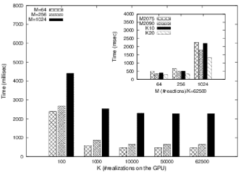
From these experiments, we can draw several conclusions. First, when the number of reactions $M$ increases, the execution time increases. However, when the number $K$ of realizations increases the execution time decreases which means that the GPU is more efficiently used and that our algorithm exploits more efficiently the GPU architecture.

These experiments also show that our GPU/AR algorithm is a scalable algorithm: the execution time decreases when using more powerfull GPU cards. For example, for $M=1024$ the execution time is 2277.18 msec on a M2075 GPU Card, and decreases to 1326.78 msec (41.73%) on a K20 GPU Cards, This means that our GPU/AR algorithm will immediately benefits from more efficient GPU cards. This also ensures its perenity for future GPU cards.

8 Discussion

Stochastic simulation in the new age of systems biology is facing the challenge of dealing with large systems characterized by an increasing number of reactions, and the need to run more and more realizations of this model.

It is well-known that the heart of the SSA algorithm, namely the selection of the next reaction to occur, is the most computationally costly part of the algorithm. To the best of our knowledge, every implemtentations are based on the inversion transform method, which needed a non deterministic number of steps obviously impacting a parallel implementation in order to tackle many realizations in parallel. Most of the SSA implementations on GPUs implement each realizations as a kernel, with the restrictions imposes to each instance of a kernel by the GPU hardware.

Here we propose a new direction of efforts that fully parallelize all the realizations of the SSA on the GPU. We propose to use an acceptance-rejection algorithm to select the next reaction to occur for $K$ parallel realizations.

We show that our algorithm: i) is well adapted to a GPU implementation, ii) is very accurate (MSE values between a given propensity distribution and the distribution of the observed generated propensities), iii) allows to select the next reaction to occur for 65536 realizations using a one-dimensional geomery of grid of blocks, iv) is scalable, meaning that our GPU-AR algorithm will benefit from more powerfull GPU cards to be released in the future.

Our algorithm uses GPU memory for the uniform random generator (one array of size $K\times M$ in this paper), the propensities values for each of the $K$ realizations (one array of size $K\times M$) and an integer array of size $K$ in order to store, at each kernel call, the index of the next reaction to occur. The rest of the computation used the shared memory (two arrays of size $M$, the number of reactions).

So our algorithm leaves some global GPU memory free for other optimizations.

For the purpose of being pedagogical we present a version that uses a maximum of $M=1024$ reactions of the model under consideration, and uses a 1D-dimensional geometry for the blocks of $M$ threads. However, if $M$ is larger it is possible to adapt the algorithm in order to use $w={M\over NumberOfThreadsPerBlock}$ blocks for the election step and modify the reduction used for the selection step. Moreover, with a 2D-dimensional grid of blocks it is possible to extend the number of realizations in parallel. Depending on the GPU card and its global memory, we succeed in running one millions of realizations in parallel (data not shown).

In order to address the widest audience, we present only the heart of the SSA that we propose to change, without embedding it in a complete implementation that could obscure the main idea. We hope that it will allows its implementation in current SSA algorithm with the benefit of using already implemented optimizations or data structures.

Acknowledgement

We would like to thank the NVIDIA Technology Center (PSG Cluster) for providing access to K10 and K20 GPU Cards.

References

- [1] Harley H. McAdams and Adam Arkin. Stochastic mechanisms in gene expression. Proc Natl Acad Sci U S A., 94(3):814–819, 1997.
- [2] Thattai Mukund and Alexander van Oudenaarden. Intrinsic noise in gene regulatory networks. Proc Natl Acad Sci U S A., 98(15):8614–8619, 2001.
- [3] Johan Paulsson. Summing up the noise in gene networks. Nature, 427:415–418, 2004.
- [4] Fiona Achcar, Jean-Michel Camadro, and Denis Mestivier. A boolean probabilistic model of metabolic adaptation to oxygen in relation to iron homeostasis and oxidative stress. BMC Systems Biology, 5:51, 2011.
- [5] D. Endy and R. Brent. Modelling cellular behavior. Nature, 409(6818):391–5, Jan 2001.
- [6] A. Arkin, J. Ross, and H.H. MacAdams. Stochastic kinetic analysis of developmental pathway bifurcation in phage lambda-infected escherichia coli cells. Genetics, 149(4):1633–48, 1998.
- [7] Daniel T. Gillespie. A general method for numerically simulating the stochastic time evolution of coupled chemical reactions. Journal of Computational Physics, 22(4):403–434, December 1976.
- [8] Daniel T. Gillespie. Exact stochastic simulation of coupled chemical reactions. The Journal of Physical Chemistry, 81(25):2340–2361, 1977.
- [9] J. Pahle. Biochemical simulations: stochastic, approximate stochastic and hybrid approaches. Briefings in Bioinformatics, 10(1):53–64, January 2009. doi:10.1093/bib/bbn050.
- [10] Nicolas Le Novère and Thomas Simon Shimizu. Stochsim: modelling of stochastic biomolecular processes. Bioinformatics, 17(6):575–6, 2001.
- [11] Yanxiang Zhou, Juliane Liepe, Xia Sheng, and Michael P.H. Stumpf. Gpu accerelerated biochemical network simulation. Bioinformatics, 27(6):874–876, 2011.
- [12] Gautier Stoll, Eric Viara, Emmanuel Barillot, and Laurence Calzone. Continuous time boolean modeling for biological signaling: application of gillespie algorithm. BMC Systems Biology, 6:116, 2012.
- [13] Ivan Komarov and M. D’Souza Roshan. Accelerating the gillespie exact stochastic simulation algoriothm using hybrid parallel execution on graphics processing units. PLoSOne, 7(11):e46693, November 2012. doi:10.371/journal.pone.0046693.
- [14] Hong Li, Yang Cao, Linda R. Petzold, and Daniel T. Gillespie. Algorithms and software for stochastic simulation of biochemical reacting systems. Biotechnol. Prog., 24(1):56–61, 2008.
- [15] Michael A. Gibson and Jehoshua Bruck. Efficient exact stochastic simulation of chemical systems with many species and many channels. Journal of Physical Chemistry A, 104(9):1876–1889, 2000.
- [16] Y. Cao, H. Li, and L. Petzold. Efficient formulation of the stochastic simulation algorithm for chemically reaction systems. J Chem Phys, 121(9):4059–4067, 2004.
- [17] James M. McCollum, Gregory D. Peterson, Chris D. Cox, Michael L. Simpson, and Nigiza F. Samatova. The sorting direct method for stochastic simulation of biochemical systems with varying reaction execution behavior. Comput. Biol. Chem., 30(1):39–49, February 2006.
- [18] Li Hong and Linda Petzold. Tech. report ”logarithmic direct method for discrete stochastic simulation of chemically reacting systems”. 2006.
- [19] Colin S. Gillespie. Stochastic simulation of chemically reacting systems using multi-core processors. J. Chem. Phys., 136(1):014101, 2012.
- [20] Daniel T. Gillespie, Andreas Hellander, and Linda R. Petzold. Perspective: Stochastic algorithms for chemical kinetics. The Journal of Chemical Physics, 138:170901, 2013.
- [21] Hong Li and Linda L. Petzold. Efficient parallelization of stochastic simulation algorithm for chemically reacting systems on the graphics processing unit. The International Journal of High Performance Computing Applications, 24:107–116, 2009.
- [22] Tianhai Tian and Kevin Burrage. Parallel implementation of stochastic simulation of large-scale cellular processes. In Proceedings of the Eight International Conference on High-Performance Computing in Asia-Pacific Region (HPCA-SIA’05), pages 621–626. 2005.
- [23] Kevin Burrage, Pamela M. Burrage, N. Hamilton, and Tianhai Tian. Compute-intensive simulations for cellular models. In Hoboken N.J., editor, Parallel Computing for Bioinformatics and Computational Biology: Models, Enabling Technologies, and Case Studies, pages 79–119. Wiley Interscience, New York, 1995.
- [24] Guido Klingbeil, Radek Erban, Mike Giles, and Philip K. Maini. Stochsimgpu: parallel stochastic simulation for the systems biology toolbox 2 for matlab. Bioinformatics, 27(8):1170–1, 2011.
- [25] Robert Farber. CUDA Application Design and Development. Morgan Kaufmann, 2011.
- [26] Jason Sanders and Edward Kandrot. CUDA by example. Addison-Wesley Professional, 2010.
- [27] R Core Team. R: A Language and Environment for Statistical Computing. R Foundation for Statistical Computing, Vienna, Austria, 2013.
- [28] Michal Januszewski and Marcin Kostur. Accelerating numerical solution of stochastic differential equations with cuda. Computer Physics Communications, 181(1):183–188, January 2010.