Transport through quasi-one-dimensional wires with correlated disorder

Abstract

We study transport properties of bulk-disordered quasi-one-dimensional (Q1D) wires paying main attention to the role of long-range correlations embedded into the disorder. First, we show that for stratified disorder for which the disorder is the same for all individual chains forming the Q1D wire, the transport properties can be analytically described provided the disorder is weak. When the disorder in every chain is not the same, however, has the same binary correlator, the general theory is absent. Thus, we consider the case when only one channel is open and all others are closed. For this situation we suggest a semi-analytical approach which is quite effective for the description of the total transmission coefficient. Our numerical data confirm the validity of our approach. Such Q1D disordered structures with anomalous transport properties can be the subject of an experimental study.

I Introduction

Recently, much attention has been paid to the problem of correlated disorder in one-dimensional (1D) systems (see for example, Ref. [IKM12, ] and references therein). As is known, in 1D models with white-noise disorder all eigenstates are localized in infinitely large samples, independently on the strength of disorder A58 ; ATAF80 ; LR85 . Although this result, known as the Anderson localization A10 , was rigorously proved for continuous potentials long ago, one has to note that for the tight-binding and Kronig-Penney models the presence of discrete resonances do not allow to treat the problem of localization rigorously for any value of energy inside the energy bands. This fact leads to the failure of the single-parameter scaling (SPS)ATAF80 according to which all transport properties of finite samples depend on the ratio of the actual sample size to the localization length defined in the limit of infinitely large samples. On the other hand, the energy intervals where the SPS fails are typically small and in real applications may be neglected.

As recently argued in Refs. [SIZC11, ; HIM13, ], outside the resonances the analytical results for the transmission coefficient and its variance, obtained for 1D continuous random potentials, can be safely used for tight-binding and Kronig-Penny models as well, provided the energy is not too close to the resonances. Moreover, it was shown that with specific methods one can effectively modify the theory and describe the global properties of the transmission within the whole energy region, including the resonance regions HIM13 .

For a long time the localization properties of weakly random potentials in the presence of correlations (colored-noise potentials) were discussed scarcely, in spite of the fact that the results developed for continuous 1D potentials have been obtained in the general form LGP88 , allowing to analyze the influence of both short and long-range correlations (see discussion in Ref. [IKM12, ]). The interest in the problem of localization for colored-noise potentials has been triggered by numerical studies of discrete dimer models for which the onset of delocalization has been observed numerically F89 ; DWP90 . Later it was understood that such delocalization emerging for discrete values of energies does not contradict the general statement of the theory of localization according to which delocalization is not possible for 1D disordered potentials. Nevertheless, since in reality the size of disordered samples is always finite, one can speak about an effective delocalization within some intervals of energy. Then, the coexistence of localized and delocalized eigenstates can be controlled by the specific choice of correlations. This non-trivial possibility to control localization properties due to specific correlations has led to intensive studies of anomalous transport properties in colored-noise potentials.

One of the results of studies of tight-binding models with colored-noise disorder is the discovery that long-range correlations can lead to vanishing Lyapunov exponent in a finite range of energy inside allowed energy bands IK99 ; KI99 . Although this result is obtained for weak disorder in the first-order perturbation theory, one can speak about the emergence of effective mobility edges dividing the regions with localized and extended states. The theoretical predictions of arranging narrow energy windows with perfect transmission in a desirable range of energy has been experimentally confirmed in microwave experiments with point-like scatterers inserted into one-channel waveguides KIKS00 ; KIKSU02 . Alternatively, it was shown that with long-range correlations one can strongly enhance the localization even when the strength of disorder is weak KIK08 . The important point is that such localization of eigenstates can be achieved in quite narrow energy regions, thus resulting in a strong selective reflection of scattering waves. Both numerical and experimental results have demonstrated robust anomalous properties of scattering even in disordered samples of relatively small size.

It should be stressed that apart from specific colored-noise potentials that can be experimentally arranged, there are many physical situations where long-range correlations are not avoidable and have to be taken into account. One of such situations occurs in experiments of 1D optical lattices with interacting bosons (see for example [So07, ; Co08, ; Ro08, ]).

In contrast to the problem of correlated disorder in 1D systems for which the theory is practically developed, the transport properties of Q1D systems with colored noise are not well understood. Among the setups studied in this direction one can mention the tight-binding Anderson model with two-coupled chains BK07 , the models with stratified or layered disorder IM05 ; IM04 , and multi-mode waveguides with long-range correlations in surface profiles IM03 ; IM05 .

The aim of this presentation is to contribute to the theory of correlated disorder in the Q1D geometry. Specifically, we consider the Q1D model of the Anderson type in correspondence with the results obtained in the theory of 1D disordered models. As the first step we analyze the situation for which the scattering potential has specific long-range correlations in the longitudinal $x-$direction, however, does not depend on the transverse $y-$coordinate. As is shown in Ref. [IM05, ], for such stratified disorder the problem can be solved analytically by the reduction of the Q1D scattering problem to the analysis of the scattering along $N$ independent 1D channels. Specifically, the independence of the disorder on the transverse coordinate allows one to reduce the model to a coset of non-interacting channels characterized by different localization lengths IM03 ; TI06 . Note that since now the total conductance is a complicated combination of partial 1D conductances, the concept of the single parameter scaling is not valid IM05 ; IM04 .

In our study we explicitly show, both analytically and numerically, that long-range correlations in Q1D wires with stratified disorder can produce a non-monotonic step-wise energy-dependent conductance. Numerical data indicate that by introducing an additional white-noise disorder in the transverse direction the effect of long-range longitudinal correlations is strongly suppressed, however, it practically remains unaffected in the channel with the lowest index.

This paper is organized as follows. In the next Section we define the model of Q1D wire and give basic relations for the characterization of scattering properties. Specifically, we show how the transmission though Q1D wires with stratified disorder can be explained in terms of the independent partial transmission coefficients corresponding to the 1D wires composing the Q1D structure. In Section III we explain the approach according to which we numerically compute the scattering properties of the Q1D correlated wires, based on an effective non-Hermitian Hamiltonian describing the scattering. Then, we verify our analytical predictions by comparing them with numerical data, and show that for a special choice of the correlated disorder the conductance shows a highly unexpected step-wise energy-dependence. Finally, in Section VI we draw our conclusions.

II Model and scattering setup

The model consists of a rectangular array of sites of length $N$ and width $M\ll N$, with nearest neighbor couplings, see Fig. 1. The Hamiltonian corresponding to this setup has the following form,

$$\left<n,m\left|H\right|n^{\prime},m^{\prime}\right>=\epsilon_{nm}\delta_{nn^{\prime}}\delta_{mm^{\prime}}-v(\delta_{nn^{\prime}}\delta_{m,m^{\prime}+1}$$

$$+\ \delta_{nn^{\prime}}\delta_{m,m^{\prime}-1}+\delta_{n,n^{\prime}+1}\delta_{mm^{\prime}}+\delta_{n,n^{\prime}-1}\delta_{mm^{\prime}})\ .$$ (1)

The on-site entries $\epsilon_{nm}$ are assumed to be random numbers whose statistical properties will be specified below, while the coupling amplitudes $v$ between sites are considered to be constant. The disordered wire is connected to semi-infinite tight-binding leads of width $M$ marked in Fig. 1 by open circles. In the leads, for $n\leq 0$ and $n\geq N$, the disorder is absent and the coupling amplitudes between the sites in the leads are also fixed to $v$.

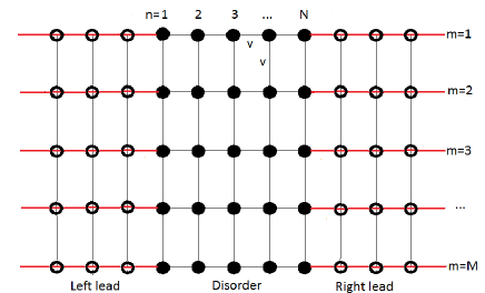
Figure 1: (Color online) Disordered Q1D wire of length $N$ and width $M$ connected at both ends to semi-infinite ideal leads.

The corresponding stationary Schrödinger equation for the eigenstates $\psi_{nm}$ of energy $E$ reads,

$$v(\psi_{n,m+1}+\psi_{n,m-1}+\psi_{n+1,m}+\psi_{n-1,m})=\left(E-\epsilon_{nm}\right)\psi_{nm}\ .$$ (2)

Without disorder, $\epsilon_{nm}=0$, the solution $\psi_{nm}$ are plane waves with wave number $\mu_{q}$ in the transverse direction. In the following, the index $q=1,\dots,M$ is treated as the channel (or mode) number. In our model we assume zero boundary conditions in the transverse direction, $\psi_{n,0}=\psi_{n,M+1}=0$, therefore, the dispersion relation takes the form,

$$2v\cos\mu_{q}=E-2v\cos\left(\frac{\pi q}{M+1}\right)\ ,\quad q=1,\dots,M\ .$$ (3)

From this relation one can see that the $q-$th channel is open as along as the energy fulfills the condition inside the interval

$$-2v\leq E-2v\cos\left(\frac{\pi q}{M+1}\right)\leq 2v\ ,$$ (4)

and outside it $\mu_{q}$ becomes imaginary. In fact, the latter equation determines the number $M_{1}(E)$ of open modes in dependence of the energy. For example, at the band center, $E=0$, all modes are open and $M_{1}=M$. While for $|E|<1+\cos\left(\pi/M+1\right)$ all modes are closed. Taking into account that

$$\cos\left(\frac{\pi q_{1}}{M+1}\right)>\cos\left(\frac{\pi q_{2}}{M+1}\right)$$

for $q_{2}>q_{1}$, one can obtain the expression for the number of open modes in terms of the energy and channel number $q$,

$$M_{1}=\left\{\begin{array}[]{lcc}q&\mbox{if}&\cos\left(\frac{(q+1)\pi}{M+1}\right)<\frac{|E|}{2v}-1<\cos\left(\frac{q\pi}{M+1}\right)\\ 0&\mbox{if}&\frac{|E|}{2v}>1+\cos\left(\frac{\pi}{M+1}\right)\end{array}\right..$$ (7)

III Non-Hermitian Hamiltonian approach

In order to analyze transport properties of our model in what follows we use the non-Hermitian Hamiltonian approach (see for example [MW69, ; SZ92, ; VZ05, ; Suren2, ]). The key point of this approach is based on the projection of the total Hermitian Hamiltonian $\mathcal{H}$ (disordered part plus leads, see Eq. (II)) onto the basis defined by the Hamiltonian $H^{(int)}$ describing the properties of the closed model (only disordered part, see Fig. 1). In this way the leads are considered as a continuum to which the disordered part is coupled according to given boundary conditions. The knowledge of the effective Hamiltonian $H^{(int)}$ allows one to construct the scattering matrix and, as a result, all transport properties can be obtained.

For our model the non-Hermitian Hamiltonian expressed in the site basis $|n,m\rangle$ has the following form,

$$\langle n,m|\mathcal{H}(E)|n^{\prime},m^{\prime}\rangle=\langle n,m|H^{(int)}|n^{\prime},m^{\prime}\rangle$$

$$-\sum^{M_{1}}_{q=1}\mbox{e}^{i\mu_{q}}\left(\gamma_{L}\delta_{n1}+\gamma_{R}\delta_{nN}\right)\delta_{nn^{\prime}}P_{qm^{\prime}}P_{qm}\ .$$ (8)

Here $H^{(int)}$ is the Hermitian Hamiltonian of the internal system, while the second term in the right hand side corresponds to the coupling of the internal system to the leads. In the general case the coupling is characterized by two parameters, $\gamma_{L}$ and $\gamma_{R}$, with $L$ and $R$ denoting the left and right leads, respectively. In our study, for simplicity, we assume symmetric couplings, $\gamma_{L}=\gamma_{R}=\gamma$. As is defined above, $\mu_{q}$ stands for the wave number at the $q-$th channel and is related to the energy $E$ through the dispersion relation (3). The elements $P_{ij}$ in Eq. (8) are nothing but the basis states in which the Hamiltonian $H^{(int)}$ is presented. In fact, they are eigenstates of this Hamiltonian in the absence of disorder,

$$P_{ij} = \sqrt{\frac{2}{M+1}}\sin\left(\frac{\pi ij}{M+1}\right).$$ (9)

Equation (8) can be written in matrix form as follows,

$${\bf\mathcal{H}}(E)={\bf H^{(int)}}+2\pi{\bf A}{\bf Q}(E){\bf A}^{T}-i\pi{\bf A}{\bf A}^{T}\ .$$ (10)

Here ${\bf H^{(int)}}$ is the $NM\times NM$ Hermitian matrix with ordered matrix elements $\Big{\langle}n,m\left|H^{int}(E)\right|n^{\prime},m^{\prime}\Big{\rangle}$. The second Hermitian and third non-Hermitian terms in the right hand side of Eq. (10) represent the real and imaginary parts of the coupling to the leads, respectively. As for the coupling matrix ${\bf A}$ of size $MN\times 2M_{1}$, it is composed by the ordered coupling amplitudes ${\bf A}=\{A^{(Lq)}_{mn},A^{(Rq)}_{mn}\}$ between the internal states $|n,m\rangle$ and open left and right channels $Lq$ and $Rq$, respectively. Thus, the coupling amplitudes are given by

$$A^{Lq}_{mn} = (\gamma_{L}/\pi)^{1/2}\sqrt{\sin\mu_{q}}P_{qm}\delta_{n1}\ ,$$ (11)

$$A^{Rq}_{mn} = (\gamma_{R}/\pi)^{1/2}\sqrt{\sin\mu_{q}}P_{qm}\delta_{nN}\ .$$

${\bf Q}(E)$ is the $2M_{1}\times 2M_{1}$ diagonal matrix with real elements ordered as $\{Q_{1},Q_{2},\dots,Q_{M_{1}},Q_{1},Q_{2},\dots,Q_{M_{1}}\}$, where

$$Q_{q}(E)=-\left(\cot\mu_{q}\right)/2,\ \ q=1,\dots,M_{1}(E).$$ (12)

Now, from the effective non-Hermitian Hamiltonian we can pass to the scattering ${\bf S}$-matrix written in the channel space,

$${\bf S}=\left(\begin{array}[]{cc}{\bf t}&{\bf r^{\prime}}\\ {\bf r}&{\bf t^{\prime}}\end{array}\right)=\frac{1+{\bf{\cal C}}^{{\dagger}}{\bf{\cal K}}}{1+{\bf{\cal C}{\cal K}}}\ ,$$ (13)

where ${\bf t}$, ${\bf t^{\prime}}$, ${\bf r}$, and ${\bf r^{\prime}}$ are $M_{1}\times M_{1}$ transmission and reflection matrices. Below, we chose the coupling parameter $\gamma$ in such a way that the transmission in each channel is maximal. This means that we consider the so-called perfect coupling for which the average scattering matrix is zero $\langle S\rangle=0$. In our case, both for the 1D model with $M=1$ and for the Q1D model with $M>1$, the perfect coupling corresponds to $\gamma\approx v$.Suren2

It can be shown that the matrix ${\bf{\cal C}}$ in Eq. (13) of size $2M_{1}\times 2M_{1}$ has the following structure,

$${\bf{\cal C}}=i\pi-2\pi{\bf Q}(E).$$

As for the reaction matrix ${\bf{\cal K}}$ (of the same size $2M_{1}\times 2M_{1}$), its matrix elements are defined by

$${\cal K}_{ab}(E) = \sum_{nm}\frac{\widehat{A}^{(a)}_{nm}\widehat{A}^{(b)}_{nm}}{E-E_{nm}}\ ,$$ (14)

$$\widehat{A}^{(a,b)}_{nm} = \sum_{rs}A^{(a,b)}_{rs}\psi_{rs}(E_{nm})\ .$$

Here, $\psi_{rs}$ are the components of the eigenvector of the matrix $\bf{H^{int}}$ having the eigenvalue $E_{nm}$, and we have introduced the channel index $a,b\equiv cq$ that indicates which lead $c=L,R$ and mode $q$ we refer to. Once the $S$-matrix is known one can calculate the dimensionless conductance $g=\left(2e^{2}/h\right)T$, where $T=\mbox{Tr}(tt^{\dagger})$ is the transmission coefficientLandauer , with $e$ as the charge of the electron and $h$ as the Planck constant.

It should be noted that at the band center the relation (10) reduces to the simple form,

$${\bf\mathcal{H}}={\bf H^{(int)}}-i\pi{\bf A}{\bf A}^{T},$$

in which the coupling to continuum is described by the imaginary term only. In addition, in the 1D case the scattering matrix (13) takes the well known form,

$${\bf S}=\frac{1-i\pi{\bf{\cal K}}}{1+i\pi{\bf{\cal K}}}\ .$$

IV correlated stratified disorder

IV.1 Analytical results

In this Section we consider the so-called stratified disorder for which the potential is independent of the transverse coordinate quantized by the index $m$, i.e.

$$\epsilon_{n1}=\epsilon_{n2}=\dots=\epsilon_{nM}\equiv\epsilon_{n}.$$ (15)

In this case our model can be reduced to a set of $M$ 1D independent chains which are nothing but 1D tight-binding Anderson modelsIM05 . To show this, first, we rewrite the Schrödinger equation (2) in the matrix form,

$${\bf a}^{(n-1)}+{\bf a}^{(n+1)}=\left({E}-{\bf B}^{(n)}-{\bf C}\right){\bf a}^{(n)}\ ,$$ (16)

where ${\bf a}^{(n)}$ is the vector with components $\psi_{nm}$ ($m=1,\dots,M$). Here ${\bf B}^{(n)}$ and ${\bf C}$ are $M\times M$ matrices with elements given by

$$B^{(n)}_{ij} = \epsilon_{nj}\delta_{ij}\ ,$$

$$C_{ij} = v(\delta_{i,j+1}+\delta_{i,j-1})\ .$$ (17)

Then, we pass to a new unperturbed basis through the transformation,

$${\bf b}^{(n)} = {\bf P}{\bf a}^{(n)}\ ,$$ (18)

where the columns of the matrix ${\bf P}$ are the eigenvectors of the Hamiltonian matrix ${\bf C}$ that correspond to the 1D Anderson model of size $M$ with vanishing disorder, $\epsilon_{i}=0$, and zero boundary conditions. Note that the corresponding eigenvectors and eigenvalues are analytically known. In this representation the Schrödinger equation (16) takes the form,

$${\bf b}^{(n+1)}+{\bf b}^{(n-1)}=\left(E-{\bf P}^{T}{\bf B}^{(n)}{\bf P}-{\bf D}\right){\bf b}^{(n)}\ ,$$ (19)

where the elements of the $M\times M$ matrix ${\bf D}$ are given by

$$D_{ij} = 2v\cos\left(\frac{\pi i}{M+1}\right)\delta_{ij},$$ (20)

while the elements of the $M\times M$ matrix $\bf P$ are given by Eq. (8).

For the stratified disorder Eqs. (19) become uncoupled since ${\bf P}^{T}{\bf B}^{(n)}{\bf P}={\bf B}^{(n)}$ is a diagonal matrix. Hence, the Q1D Anderson model is reduced to a set of $M$ 1D chains, where the energy for each chain is given by

$$E_{q}=E-2v\cos\left(\frac{\pi q}{M+1}\right)\ ,\quad q=1,\dots,M\ .$$ (21)

Let us now specify the properties of the stratified disorder. First, we assume zero mean and small variance $\sigma^{2}$ of the site energies,

$$\langle\epsilon_{n}\rangle=0\ ,\quad\sigma^{2}=\langle\epsilon^{2}_{n}\rangle\ll 1\ ,$$ (22)

where $\langle\cdots\rangle$ denotes the average over different realizations of disorder. Apart from that, we assume that the statistical properties of disorder are defined by the two-point correlator describing the long-range correlations. Therefore, an additional ingredient of the disorder is the specific form of the normalized binary correlator,

$$\chi(k)=\frac{\left<\epsilon_{n}\epsilon_{n+k}\right>}{\sigma^{2}},$$ (23)

to be defined below.

Since our model with the stratified disorder can be rigorously reduced to a set of $M$ 1D chains, one can try to apply the theory of 1D localization developed for continuous potentials. According to this theory for weak disorder and in the limit $N\rightarrow\infty$, the eigenstates $b^{(n)}_{q}$ (in our case, the components of the vectors ${\bf b}^{(n)}$, see Eq. (19)) are exponentially localized with the characteristic length $l^{(q)}_{\infty}$ related to the $q-$th channel. As is known, the inverse localization length can be defined in terms of the Lyapunov exponent $\lambda_{q}$, and the analytical expression for the latter has the following form (see for example Ref. [IKM12, ]),

$$\lambda_{q} \equiv \frac{1}{l^{(q)}_{\infty}}=\frac{\sigma^{2}}{8\sin^{2}\mu_{q}}W(2\mu_{q})\ ,$$

$$W(2\mu_{q}) = 1+2\sum^{\infty}_{k=1}\chi(k)\cos{2\mu_{q}k}\ .$$ (24)

As one can see, the correlation properties of the random sequence $\{\epsilon_{n}\}$ are entirely defined by the power spectrum $W(\mu)$ of the binary correlator. Note that this result is correct for weak disorder; as for the higher moments of the correlations they may contribute to the localization length only in the next order of perturbation theory in the disorder parameter $\sigma^{2}$. Note that for white noise disorder, we have $W(2\mu_{q})=1$.

Now we focus on the problem of scattering through the disordered region represented by full circles in Fig. 1. Since for the stratified disorder the transmission along every 1D channel is independent from those along the other channels, the total transmission coefficient $T$ can be expressed as the sum of partial coefficients $T_{q}$ corresponding to the propagation of incident plane waves along the $q-$th independent channels,

$$T(E)=\sum^{M_{1}}_{q=1}T_{q}(E)\ .$$ (25)

This expression agrees with the Landauer concept of conductance Landauer . Here $M_{1}(E)$ is the number of open modes in the leads given by Eq. (7).

Above we announced that we plan to use the analytical results developed for 1D continuous models. However, the model under consideration is a discrete model for which the theoretical analysis is restricted due to the presence of resonances in the energy space (see for example [IKM12, ; THI12, ] and references therein). Specifically, there are no rigorous results for the probability distribution of $T$, or equivalently, for the corresponding moments for any energy inside the allowed energy band. To the contrary, for continuous random potentials with weak disorder the problem of scattering through finite 1D wires was rigorously solved by various analytical approaches IKM12 ; LGP88 . In particular, there is an exact expression for the average transmission coefficient in terms on the ratio of the localization length $l_{\infty}$ to the length $N$ of the sample IKM12 ; LGP88 ,

$$\langle T_{q}\rangle = \sqrt{\frac{2x^{3}_{q}}{\pi}}\mbox{exp}\left(-\frac{1}{2x_{q}}\right)\int^{\infty}_{0}\frac{z^{2}}{\cosh z}\mbox{exp}\left(-\frac{z^{2}x_{q}}{2}\right)dz,$$

$$x_{q} = l^{(q)}_{\infty}/N\ .$$ (26)

In Eq. (26), we have added the index $q$ in order to indicate to which channel we are referring to. Here, the brackets stand for the average over a number of different realizations of the correlated disorder.

As was found in Ref. [SIZC11, ], the latter expression turns out to be very good even for the 1D tight-binding Anderson model, provided the energy values are not very close to the resonances. Moreover, recently a new approach has been developed in Ref. [HIM13, ] allowing one to modify the standard perturbation theory in such a way that it gives good results also at the resonant energies. In particular, it was shown that Eq. (26) still gives a good description of numerical results at the resonances, provided the expression for the localization length takes into account the influence of these resonances. Thus, relation (26), together with Eqs. (IV.1) and (25), give us the possibility to obtain the expression for the transmission coefficient $\langle T(E)\rangle$ in dependence on the model parameters. Below we verify the validity of Eq. (26) by comparing it with numerical data.

IV.2 Numerical data

Since the localization length $l^{(q)}_{\infty}$ of any $q-$th conducting channel is fully determined by Eq. (IV.1), if the power spectrum $W(2\mu_{q})$ vanishes within some energy window, the corresponding channel will be fully transparent in this energy interval IK99 ; KI99 ; IM09 . This prediction has been confirmed both numerically and experimentally for the 1D Anderson model (see details and references in Ref. [IKM12, ]). Here our interest is on how this effect can be seen in the Q1D model with the stratified disorder. To do this, we choose the following form of the binary correlator,

$$\chi(k)=\frac{1}{2k(\mu_{R}-\mu_{L})}\left(\sin 2\mu_{R}k-\sin 2\mu_{L}k\right)\ .$$ (27)

As one can see, this correlator exhibits a power law decay which is typical for long-range correlated disorder. It can be shown that the correlator (27) results in the step-wise power spectrum,

$$W(E_{q})=\left\{\begin{array}[]{ll}W_{0}&\ \mbox{if}\ E_{L}\leq\left|E_{q}\right|\leq E_{R}\\ 0&\ \mbox{if}\ |E_{q}|<E_{L}\ \mbox{or}\ E_{R}<|E_{q}|\leq 2v\end{array}\right..$$ (30)

Here, $\mu_{L}$ and $\mu_{R}$ are related to $E_{L}$ and $E_{R}$ through the dispersion law for the 1D system, $E=2\cos\mu$, and $W_{0}$ is determined by the normalization condition $\int^{\pi/2}_{0}W(\mu)d\mu=\pi/2$ (see details in Ref. [IKM12, ]). Note that we have omitted the transverse index $m$ since each chain has the same disorder sequence $\epsilon_{n}$. In our numerical simulations we consider the following fixed values: $E_{L}=0.4$, $E_{R}=1.3$, $\sigma^{2}=0.02$, and $v=1$.

Correlations with the power spectrum (30) have been already used in the literature to control the transport properties of 1D systems IM09 ; ivan2 . In Fig. 2 we demonstrate these properties by considering our model with one chain only, $M=1$. Specifically, we present the analytical expression for the Lyapunov exponent (IV.1), together with the predicted and actual dependence of the transmission coefficient $\langle T\rangle$, see Eq. (26). One can see a good correspondence with the data showing the expected windows of transparency in dependence of the energy $E$.

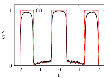
Figure 2: (Color online) (a) Rescaled Lyapunov exponent $\lambda N$ as a function of the energy $E$ for one chain, $M=1$. The correlated disorder has been fixed by the step-wise power spectrum of Eq. (30) with $E_{L}=0.4$, $E_{R}=1.3$, $\sigma^{2}=0.02$, and $v=1$. (b) Average transmission coefficient $\left\langle T\right\rangle$ as a function of $E$. The continuous curve corresponds to numerical data while the dashed one is the theoretical prediction from Eqs. (IV.1-26). The average is taken over 100 realizations of disorder for a disordered region of length $N=300$.

For the Q1D model with the stratified disorder the scenario is much more complicated. Indeed, for any of the $q-$th channels the windows of transparency are defined by the energy shifted in accordance with Eq. (21). Specifically, for each channel there are three transparent energy windows given by Eq. (30). Outside of these windows the transmission vanishes due to the chosen type of correlations. Thus, the total transmission is obtained by the overlap of the energy dependencies corresponding to each channel. One can show that the average transmission coefficient is approximately defined by the integer number due to the following expression,

$$N_{c}(E) = \sum^{M}_{q=1}\Big{(}\Theta[E_{q}+E_{L}]-\Theta[E_{q}-E_{L}]+\Theta[E_{q}-E_{R}]$$ (31)

$$- \Theta[E_{q}+E_{R}]+\Theta[E_{q}+2v]-\Theta[E_{q}-2v]\Big{)},$$

with $\Theta[x]$ as the Heaviside step function. The resulting step-wise behavior is shown in Figs. 3. Notice that the maximum value of the average conductance is reached, in most of the cases, in the energy region where without disorder all modes are open, therefore, the average transmission takes its maximum value $M$. The general properties of such a behavior were predicted in Ref. [IM05, ]. As one can see, the main feature of the correlated disorder is the non-monotonic dependence of the transmission in dependence on the energy.

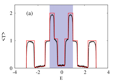
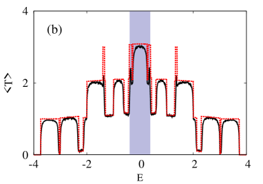
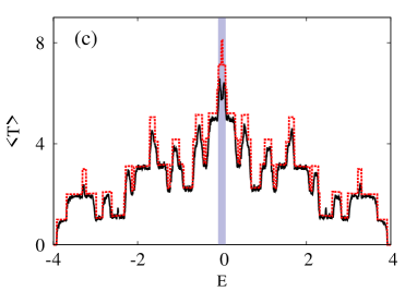
Figure 3: (Color online) Same as in Fig. 2(b) for the Q1D model with (a) $M=2$, (b) $M=5$, and (c) $M=10$. The energy window where all modes in the leads are open is shown by the shaded region.

The data presented in Figs. 3 is obtained by averaging over a large number of disorder realizations with the same kind of long-range correlations. However, from the experimental view point it is important to know whether the non-monotonic dependence of $T(E)$ can be practically seen for individual samples. To answer this question, it may be helpful to understand how the fluctuations of the transmission coefficient for an individual disordered sample of size $N$ depend on the model parameters. According to the theory of 1D disordered systems in the ballistic regime, $N/l^{(q)}_{\infty}\ll 1$, the variance of $T_{q}$ can be written as follows IKM12 ,

$$\mbox{Var}(T_{i})=4\left(\frac{N}{L^{(i)}_{\infty}}\right)^{2}+O\left(\left(\frac{N}{L^{(i)}_{\infty}}\right)^{3}\right)\ .$$ (32)

Therefore, one can expect that if the $q-$th channel is open (ballistic regime, $T_{q}\approx 1$), the fluctuations should be not very strong. On the other hand, if due to specific long-range correlations the $q-$th channel is closed (localized regime, $T_{q}\ll 1$) the fluctuations are also not important. The numerical data reported in Fig. 4 demonstrate that the non-monotonic step-wise dependence of $T(E)$ can be still detected. However, the fluctuations can wash out very narrow peaks; this can be clearly seen when the average is performed (compare with Fig. 3).

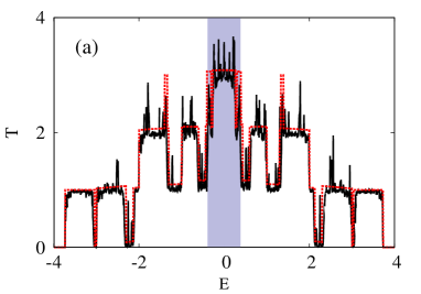
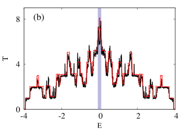
Figure 4: (Color online) Transmission coefficient $T$ as a function of $E$ for the Q1D model of length $N=300$ with (a) $M=5$ and (b) $M=10$. Continuous curves correspond to the numerical data while dashed curves are the theoretical predictions from Eqs. (IV.1-26). A single realization of disorder was used. The energy window where all modes in the leads are open is indicated by the shaded region.

V Correlated non-stratified disorder

Another important problem refers to the Q1D model (II) with the disorder having the same correlation properties in the longitudinal direction for each chain, however, with no correlations in the vertical direction. Mathematically, this means that the disorder potential depends on both transverse and longitudinal coordinates, being correlated along the sample, however, completely uncorrelated transverse to the sample. In other words, the statistical properties for the site energies are defined as follows,

$$\langle\epsilon_{nm}\rangle=0\ ,\ \ \sigma^{2}=\langle\epsilon^{2}_{nm}\rangle\ ,\ \ \chi(k)\delta_{mm^{\prime}}=\frac{\langle\epsilon_{nm}\epsilon_{n+k,m^{\prime}}\rangle}{\sigma^{2}}\ ,$$

(33)

where $\chi(k)$ is the normalized binary correlator of the site energies. As before, we assume that the disorder is weak, $\sigma^{2}\ll 1$. In the numerical calculations the specific form of the correlator is chosen according to Eq. (27) with the corresponding power spectrum (30). However, the analytical approach can be applied to systems with any form of the binary correlator $\chi(k)$.

When the correlated disorder is not stratified, the model can not be represented by a set of independent 1D systems, and the analytical solution for the localization length is known for specific cases only. It should be, however, noted that in the case of weak white-noise disorder the problem has been solved in Refs. [VG, ; VG1, ]. As for the correlated disorder, the general solution has been obtained for the two-chain model only BK07 .

Our particular interest in this Section is in the situation when one channel is open and all the others are closed. Only in this case we can suggest the phenomenological expression for the Lyapunov exponent, and make the comparison with numerical data. Thus, below we consider the Q1D model under the following conditions corresponding to this situation,

$$2v\left(1+\cos\frac{2\pi}{M+1}\right)<\left|E\right|<2v\left(1+\cos\frac{\pi}{M+1}\right),$$ (34)

where the first mode $q=1$ is open if $E>0$. Note that if $E<0$ the open mode is the last one, with $q=M$. For the two-chain model with one open channel the formula for the inverse localization length reads BK07 ,

$$\lambda(E) = \frac{1}{32\sin^{2}\mu_{q}}\left[\left<\epsilon^{2}_{n1}\right>W_{11}(2\mu_{q})+\left<\epsilon^{2}_{n2}\right>W_{22}(2\mu_{q})\right.$$ (35)

$$+ \left.2\left<\epsilon_{n1}\epsilon_{n2}\right>W_{12}(2\mu_{q})\right],$$

where $\mu_{q}$ is the wave number of the open mode ($q=1,2$). Here the power spectra $W_{ij}(\mu)$ are defined as

$$W_{ij}(\mu)=1+2\sum^{\infty}_{k=1}\chi_{ij}(k)\cos(\mu k)\ ,$$

with the binary correlators $\chi_{ij}(k)$ given by

$$\chi_{11}(k) = \frac{\langle\epsilon_{1,n}\epsilon_{1,n+k}\rangle}{\langle\epsilon^{2}_{n1}\rangle}\ ,\ \ \chi_{22}(k)=\frac{\langle\epsilon_{2,n}\epsilon_{2,n+k}\rangle}{\langle\epsilon^{2}_{n2}\rangle}\ ,$$

$$\chi_{12}(k) = \frac{\langle\epsilon_{1,n}\epsilon_{2,n+k}\rangle}{\langle\epsilon_{n1}\epsilon_{n2}\rangle}\ .$$

Formula (35) is valid for weak disorder and not very close to the critical energies where the transition from propagating to evanescent regime occurs.

Let us apply Eq. (35) to our model with two chains having the statistical properties given by Eq. (33). Therefore, $W_{ij}(2\mu_{q})=W(2\mu_{q})$, and

$$\lambda(E)=\frac{\sigma^{2}W(2\mu_{1})}{16\sin^{2}\mu_{1}}.$$ (36)

Note that the localization length is a symmetric function with respect to $E=0$. Therefore, all localization properties are the same either for $q=1$ or $q=M$.

Another analytical result, however, for the white-noise disorder reads VG1 ,

$$\lambda(E)=\frac{(3+\delta_{2,M+1})\sigma^{2}}{16(M+1)\sin^{2}\mu_{1}},$$ (37)

which is written for $M$ chains and one open channel. With the use of this expression, one can suggest the phenomenological generalization valid for the correlated disorder as well,

$$\lambda(E)=\frac{(3+\delta_{2,M+1})\sigma^{2}W(2\mu_{1})}{16(M+1)\sin^{2}\mu_{1}}.$$ (38)

Note that in the case of uncorrelated disorder, $W(2\mu_{q})=1$, the latter expression reduces to Eq. (37) and for $M=2$ the result (36) is recovered. Quite remarkable is the prediction that the inverse localization length decreases as the number of longitudinal chains $M$ increases.

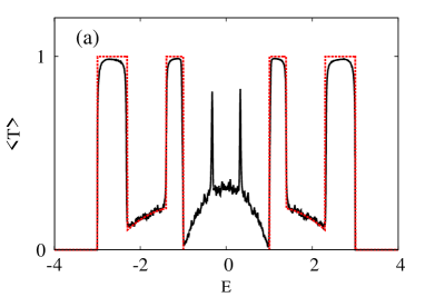
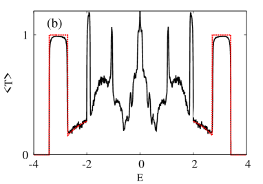
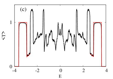
Figure 5: (Color online) Average transmission coefficient as a function of the energy for non-stratified disorder. Continuous curves represent the numerical data and dashed curves are the theoretical prediction given by Eqs. (26) and (38). The length of the system is $N=300$ with the disorder strength $\sigma^{2}=0.02$ for (a) $M=2$, (b) $M=3$, and (c) $M=4$.

It should be pointed out that here we study the case when the longitudinal and transverse hopping amplitudes are equal, see Fig. 1. Therefore, all the sub-bands (4) are overlapped. However, the expression (38) can be generalized even for the case when the transverse hopping amplitudes are not equal to the longitudinal ones, this could lead to the non-overlapping of some sub-bands. In this case one has also to take into account the influence of the evanescent modes as stated in Ref. [He, ]. Another result can be found in Ref. [ZZ, ] where the localization-delocalization transition was studied when considering the strength of the transverse hopping as an independent parameter.

Now, since only one open mode contributes to transmission, one can suggest that the expression for the average total transmission (in the energy region where only one mode is open) can be obtained by inserting the localization length defined by Eq. (38) into Eq. (26). Indeed, our numerical data presented in Figs. 5 manifest that Eq. (38) gives very good description for the total transmission coefficient in the energy regions corresponding to only one open channel. One can also see that when more than one channel is open the energy dependence of the transmission coefficient acquires a quite complicated form, thus indicating the failure of the analytical approach in the general case.

VI Conclusions

We have studied the transport properties of bulk-disordered Q1D wires paying attention to the role of long-range correlations along disordered structures of finite size. First, we have manifested that in the case of stratified disorder all transport properties can be fully explained analytically. As predicted in Ref. [IM05, ], in this case the expression for the total transmission coefficient $T$ can be presented as a sum of partial coefficients $T_{q}$ that correspond to independent 1D chains characterized by the index $q$. Since the theory of correlated disorder for 1D tight-binding models is fully developed (see for example [IKM12, ]), this allows one to incorporate the obtained results into the problem of the correlated transport for Q1D disordered systems. Our numerical data demonstrate a perfect agreement with the analytical predictions. For the numerical study we have used the approach which is based on the non-Hermitian Hamiltonians from which one can construct the scattering matrix, therefore, all transport characteristics can be extracted.

As the second step, we have analyzed the model in which the long-range correlations are taken in the same way as for the stratified disorder, however, the individual realizations of the disorder in the chains are independent from each other. Since in this case the disorder potential depends on both coordinates, the longitudinal and transverse ones, there is mixing between different channels when the waves propagate through the Q1D structure. Since the general theory is absent, we have studied the situation when one channel is open only, while $M-1$ other channels are closed. For this case the rigorous theory is also absent, however, we suggest an approach which gives a phenomenological expression for the transmission coefficient, based on the results obtained earlier for white-noise disorder. The suggested expression turns out to be very good, as the comparison with the data shows. It should be noted that such a situation when the transport in Q1D systems is practically defined by one open channel can be easily arranged experimentally.

Finally, we would like to point out that specific long-range correlations can result in a strong enhancement of the localization, even when the disorder is weak (see results, discussion, and references in Ref. [IKM12, ]). This effect is clearly seen from our numerical data that is obtained for relatively short disordered samples. Specifically, the emergence of the energy windows where the transmission coefficient vanishes or becomes very small, is a direct consequence of the enhancement of the localization. Interestingly enough, such an enhancement of localization in the selected energy windows is accompanied by the suppression of localization in the complementary energy windows within the energy bandIKM12 . Therefore, the long-range correlations can be considered as the mechanism for the redistribution of the degree of localization in the energy space. This effect can be used to manufacture devices with controlled transport properties in photonic heterostructures, semiconductor superlattices, and electron nanoconductors; among others.

- (1) F. M. Izrailev, A. A. Krokhin, and N. M. Makarov, Phys. Rep. 512, 125 (2012).
- (2) P. W. Anderson, Phys. Rev. 109, 1492 (1958).
- (3) P. W. Anderson, D. J. Thouless, E. Abrahams, and D. S. Fisher, Phys. Rev. B 22, 3519 (1980).
- (4) P. A. Lee and T. V. Ramakrishnan, Rev. Mod. Phys. 57, 287 (1985).
- (5) E. Abrahams, editor, 50 years of Anderson Localization, (World Scientific, Singapore, 2010).
- (6) I. F. Herrera-Gonzalez, F. M. Izrailev, and N. M. Makarov, Phys. Rev. E 88, 052108 (2013).
- (7) S. Sorathia, F. M. Izrailev, V. G. Zelevinsky, and G. L. Celardo, Phys. Rev. E. 86, 011142 (2012) .
- (8) I. M. Lifshitz, S. A. Gradeskul, and L. A. Patur, Introduction to the Theory of Disordered Systems (Wiley, New York, 1988).
- (9) C. Flores, J. Phys. Condens. Matter 1 8471 (1989).
- (10) D. H. Dunlap, H.-L. Wu, and P. W. Phillips, Phys. Rev. Lett. 65, 88 (1990).
- (11) F. M. Izrailev and A. A. Krokhin, Phys. Rev. Lett. 82, 4062 (1999).
- (12) A. A Krokhin and F. M. Izrailev, Ann. Phys. (Leipzig) 8, 153 (1999).
- (13) U. Kuhl, F. M. Izrailev, A. A. Krokhin, H.-J. Stöckmann, Appl. Phys. Lett. 77, 633 (2000).
- (14) A. Krokhin, F. Izrailev, U. Kuhl, H.-J. Stöckmann, S. E. Ulloa, Physica E 13, 695 (2002).
- (15) U. Kuhl, F. M. Izrailev, A. A. Krokhin, Phys. Rev. Lett. 100, 126402 (2008).
- (16) L. Sanchez-Palencia, D. Clement, P. Lugan, P. Bouyer, G. V. Shlyapnikov, and A. Aspect, Phys. Rev. Lett. 98, 210401 (2007).
- (17) J. Chabé, G. Lemarié, B. Grémaud, D. Delande, P. Szriftgiser, and J. C. Garreau, Phys. Rev. Lett. 101, 255702 (2008).
- (18) G. Roati, C. D’Errico, L. Fallani, M. Fattori, C. Fort, M. Zaccanti, G. Modugno, and M. Inguscio, Nature 453, 895 (2008).
- (19) V. M. K. Bagci and A. A. Krokhin, Phys. Rev. B 76, 134202 (2007).
- (20) F. M. Izrailev and N. M. Makarov, J. Phys. A 38, 10613 (2005).
- (21) F. M. Izrailev and N. M. Makarov, Appl. Phys. Lett. 84, 5150 (2004).
- (22) F. M. Izrailev and N. M. Makarov, Phys. Rev. B 67, 113402 (2003).
- (23) L. Tessieri and F. M. Izrailev, J. Phys. A 39, 11717 (2006).
- (24) C. Mahaux and H. A. Weidenmüller, Shell Model Approach to Nuclear Reactions (North-Holland, Amsterdam, 1969).
- (25) V. V. Sokolov and V. G. Zelevisnky, Ann. Phys. (N.Y.) 216, 323 (1992).
- (26) A. Volya and V. G. Zelevisnky, in Nuclei and Mesoscopic Physics, edited by V. G. Zelevisnky, AIP Conf. Proc. No. 777 (AIP, Melville, NY, 2005), p. 229.
- (27) S. Sorathia, Scattering properties of open systems of interacting quantum particles, PhD Thesis, Benemérita Universidad Autónoma de Puebla, Mexico, 2010.
- (28) R. Landauer, IBM J. Res. Dev. 1, 223 (1957); 32, 336 (1988); M. Buttiker, Phys. Rev. Lett. 57, 1761 (1986); IBM J. Res. Dev. 32, 317 (1988).
- (29) L. Tessieri, I. F. Herrera-González, and F. M. Izrailev, Physica E 44, 1260 (2012).
- (30) F. M. Izrailev and N. M. Makarov, Phys. Rev. Lett. 102, 203901 (2009).
- (31) U. Kuhl, F. M. Izrailev, A. A. Krokhin, and H.-J. Stöckmann, Appl. Phys. Lett. 77, 633 (2000); J. C. Hernández-Herrejón, F. M. Izrailev, and L. Tessieri, Physica E 42, 2203 (2010); I. F. Herrera-González, F. M. Izrailev, and L. Tessieri, Europhys. Lett. 90, 14001 (2010); O. Dietz, U. Kuhl, J. C. Hernández-Herrejón, and L. Tessieri, New. J. Phys. 14, 013048 (2012).
- (32) V. Gasparian, Phys. Rev. B 77, 113105 (2008).
- (33) V. Gasparian and A. Suzuki, J. Phys. Condens. Matter. 21, 405302 (2009).
- (34) J. Heinrichs, Phys. Rev. B 68, 155403 (2003).
- (35) W. Zhang, R. Yang, Y. Zhao, S. Duan, P. Zhang, and S. E. Ulloa, Phys. Rev. B 81, 214202 (2010).