Neutron Star instabilities in full General Relativity using a $\Gamma=2.75$ ideal fluid

Abstract

We present results about the effect of the use of a stiffer equation of state, namely the ideal-fluid $\Gamma=2.75$ ones, on the dynamical bar-mode instability in rapidly rotating polytropic models of neutron stars in full General Relativity. We determine the change on the critical value of the instability parameter $\beta$ for the emergence of the instability when the adiabatic index $\Gamma$ is changed from 2 to 2.75 in order to mimic the behavior of a realistic equation of state. In particular, we show that the threshold for the onset of the bar-mode instability is reduced by this change in the stiffness and give a precise quantification of the change in value of the critical parameter $\beta_{c}$. We also extend the analysis to lower values of $\beta$ and show that low-beta shear instabilities are present also in the case of matter described by a simple polytropic equation of state.

I Introduction

Non-axisymmetric deformations of rapidly rotating self-gravitating bodies are a rather generic phenomenon in nature and could appear in a variety of astrophysical scenarios like stellar core collapses Shibata and Sekiguchi (2005); Ott et al. (2005), accretion-induced collapse of white dwarfs Burrows et al. (2007), or the merger of two neutron stars Shibata et al. (2003a); Shibata et al. (2005). Over the years, a considerable amount of work has been devoted to the search of unstable deformations that, starting from an axisymmetric configuration, can lead to the formation of highly deformed rapidly rotating massive objects Shibata et al. (2000); Baiotti et al. (2007); Kruger et al. (2010); Kastaun et al. (2010); Lai and Shapiro (1995). Such deformations would lead to an intense emission of high-frequency gravitational waves (i.e. in the kHz range), potentially detectable on Earth by next-generation gravitational-wave detectors such as Advanced LIGO Harry and LIGO Scientific Collaboration (2010), Advanced VIRGO and KAGRA Somiya (2012) in the next decade LIGO Scientific Collaboration et al. (2013).

From the observational point of view, it is import to get any insight on the possible astrophysical scenarios where such instabilities (unstable deformation) are present. It is well known that rotating neutron stars are subject to non-axisymmetric instabilities for non-radial axial modes with azimuthal dependence $\mathrm{e}^{im\phi}$ (with $m=1,2,\ldots$) when the instability parameter $\beta\equiv T/|W|$ (i.e. the ratio between the kinetic rotational energy $T$ and the gravitational potential energy $W$) exceeds a critical value $\beta_{c}$. The instability parameter plays an important role in the study of the so-called dynamical bar-more instability, i.e. the $m=2$ instability which takes place when $\beta$ is larger than a threshold  Baiotti et al. (2007). Previous results for the onset of the classical bar-mode instability have already showed that the critical value $\beta_{c}$ for the onset of the instability is not an universal quantity and it is strongly influenced by the rotational profile Shibata et al. (2003b); Karino and Eriguchi (2003), by relativistic effects Shibata et al. (2000); Baiotti et al. (2007), and, in a quantitative way, by the compactness Manca et al. (2007).

However, up to now, significant evidence of their presence when realistic Equation of State (EOS) are consider is still missing. For example in Corvino et al. (2010), using the unified SLy EOS Douchin and Haensel (2001), was shown the presence of shear-instability but no sign of the classical bar-mode instability and of its critical behavior have been found. The main aim of the present work is to get more insight on the behavior of the classical bar-mode instability when the matter is described by a stiffer more realistic EOS. The investigation in the literature on its dependence on the stiffness of EOS usually focused on the values of $\Gamma$ (i.e. the adiabatic index of a polytropic EOS) in the range between $\Gamma=1$ and $\Gamma=2$ Lai and Shapiro (1995); Zink et al. (2007); Kastaun et al. (2010), while the expected value for a real neutron star is more likely to be around $\Gamma=2.75$ at least in large portions of the interior. Such a choice for the EOS has already been implemented in the past R. Oechslin et al. (2007), even quite recently Giacomazzo and Perna (2013), with the aim of maintaining the simplicity of a polytropic EOS and yet obtaining properties that resemble a more realistic case. Indeed, as it is shown in Fig. 1, a polytropic EOS with $K=30000$ and $\Gamma=2.75$ is qualitatively similar to the Shen proposal Shen et al. (1998a, b) in the density interval between $2\times 10^{13}\text{g/cm}^{3}$ and $10^{15}\text{g/cm}^{3}$. For the sake of completeness, in Fig. 1 we also report the behavior of the $\Gamma=2$ polytrope used in Baiotti et al. (2007); Manca et al. (2007) and of the unified SLy EOS Douchin and Haensel (2001) which describes the high-density cold (zero temperature) matter via a Skyrme effective potential for the nucleon-nucleon interactions Corvino et al. (2010).

The organization of this paper is as follows. In Sect. II we describe the main properties of the relativistic stellar models we investigated and briefly review the numerical setup used for their evolutions. In Sect. III we present and discuss our results, showing the features of the evolution for models that lie both above and below the threshold for the onset of the bar-mode instability and quantifying the effects of the compactness on the onset of the instability. Conclusions are finally drawn in Sect. IV. Throughout this paper we use a space-like signature $-,+,+,+$, with Greek indices running from 0 to 3, Latin indices from 1 to 3 and the standard convention for summation over repeated indices. Unless otherwise stated, all quantities are expressed in units in which $c=G=M_{\odot}=1$.

II Initial models and Numerical setup

In this work we solve the Einstein’s field equations

$$G_{\mu\nu}=8\pi T_{\mu\nu}\,,$$ (1)

where $G_{\mu\nu}$ is the Einstein tensor of the four-dimensional metric $g_{\mu\nu}$ and $T^{\mu\nu}$ is the stress-energy tensor of an ideal fluid. This can be parametrized as

$$T^{\mu\nu}=\rho\left(1+\epsilon+\frac{P}{\rho}\right)u^{\mu}u^{\nu}+Pg^{\mu\nu}\,,$$ (2)

where $\rho$ is the rest-mass density, $\epsilon$ is the specific internal energy of the matter, $P$ is the pressure and $u^{\mu}$ is the matter $4$-velocity. The evolution equations for the matter follow from the conservation laws for the energy-momentum tensor $\nabla_{\mu}T^{\mu\nu}=0$ and the baryon number $\nabla_{\mu}(\rho u^{\mu})=0$, closed by an EOS of the type $P=P(\rho,\epsilon)$.

In order to generate the initial data we evolve in this work, we use a $\Gamma$-type EOS of the form

$$P=K\rho^{\Gamma}\,,$$ (3)

where the following relation between $\epsilon$ and $\rho$ holds: $\epsilon=K\rho^{(\Gamma-1)}/(\Gamma-1)$. On the other hand, the evolution is performed using the so-called ideal-fluid ($\Gamma$-law) EOS

$$P=(\Gamma-1)\rho\epsilon\,,$$ (4)

that allows for increase of the internal energy, by shock heating, if shocks are presents. We have chosen the EOS polytropic parameters to be $\Gamma=2.75$ for the adiabatic index and $K=30000$ for the polytropic constant. This choice of parameters has the property to closely reproduce the behavior of the Shen EOS in the interior of a real neutron star (see Fig. 1). We note that the choice we make here is different from the one of our previous studies De Pietri et al. (2007); Baiotti et al. (2007); Manca et al. (2007), where we used $\Gamma=2$ and $K=100$, with the explicit intention of determining the difference that such a change implies on the onset of the bar-mode instability.

Figure 1: Diagram of the pressure $P$ vs. the energy density $e$ for two polytropic EOSs and two realistic EOS for nuclear matter, namely: (1) the Shen proposal Shen et al. (1998a, b); (2) the unified SLy prescription Douchin and Haensel (2001).

We solve the above-mentioned set of equations using the usual $3+1$ space-time decomposition, where the space-time is foliated as a tensor product of a three-space and a time coordinate $t$ (which is selected to be the $x^{0}$ coordinate). In this coordinate system the metric can be split as $g^{\mu\nu}=-n^{\mu}n^{\nu}+h^{\mu\nu}$, where $h^{\mu\nu}$ has only the spatial components different from zero and can be used to define a Riemannian metric $\gamma^{ij}=h^{ij}$ on each foliation. The vector $n^{\mu}$, that determines the direction normal to the 3-hypersurfaces of the foliation, is decomposed in terms of the lapse function $\alpha$ and the shift vector $\beta^{i}$, such that $n^{\mu}=\alpha^{-1}\cdot(1,\beta^{i})$. We also define the fluid three-velocity $v^{i}$ as the velocity measured by a local zero-angular momentum observer ($u^{i}=\alpha v^{i}-\beta^{i}$), while the Lorentz factor is $\alpha u^{0}=\sqrt{1-\gamma_{ij}v^{i}v^{j}}$. Within this formalism, the conservation of the baryon number suggests the use of the conserved variable $D=\sqrt{\gamma}\alpha u^{0}\rho$ with the property that $\int D\,d^{3}x=\text{const}$ along the time-evolution $t$.

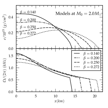
Figure 2: Density profile (top panel) and differential rotation profile (bottom panel) of some representative models among all the ones that have been evolved in this paper.

II.1 Initial Data

The initial data of our simulations are computed as stationary equilibrium solutions for axisymmetric and rapidly rotating relativistic stars in polar coordinates Stergioulas and Friedman (1995). In generating these equilibrium models we assumed that the metric describing the axisymmetric and stationary relativistic star has the form

$$ds^{2}=-e^{\mu+\nu}dt^{2}+e^{\mu-\nu}r^{2} \sin^{2}\theta(d\phi-\omega dt^{2})^{2}$$

$$+e^{2\xi}(dr^{2}+r^{2}d\theta^{2})\,,$$ (5)

where $\mu$, $\nu$, $\omega$, and $\xi$ are space-dependent metric functions. Similarly, we assume the matter to be characterized by a non-uniform angular velocity distribution of the form

$$\Omega_{c}-\Omega=\frac{1}{\hat{A}^{2}r_{e}^{2}}\bigg{[}\frac{(\Omega-\omega)r^{2}\sin^{2}\theta e^{-2\nu}}{1-(\Omega-\omega)^{2}r^{2}\sin^{2}\theta e^{-2\nu}}\bigg{]}\,,$$ (6)

where $r_{e}$ is the equatorial stellar coordinate radius, and the coefficient $\hat{A}$ is the measure of the degree of the differential rotation, which we set to be $\hat{A}=1$, in analogy with other works in the literature. Once imported onto the Cartesian grid and throughout the evolution, we compute the coordinate angular velocity $\Omega$ on the $(x,y)$ plane as,

$$\Omega=\frac{u^{\phi}}{u^{0}}=\frac{u^{y}\cos\phi-u^{x}\sin\phi}{u^{0}\sqrt{x^{2}+y^{2}}}\,.$$ (7)

Other characteristic quantities of the system such as the baryon mass $M_{0}$, the gravitational mass $M$, the internal energy $E_{\textrm{int}}$, the angular momentum $J$, the rotational kinetic energy $T$, the gravitational binding energy $W$ and the instability parameter $\beta$ are defined as Baiotti et al. (2007):

$$M_{0} \equiv\int d^{3}xD\,,$$ (8)

$$M \equiv\int d^{3}x(-2T^{0}_{0}+T^{\mu}_{\mu})\alpha\sqrt{\gamma}\,,$$ (9)

$$E_{\textrm{int}} \equiv\int d^{3}xD\varepsilon\,,$$ (10)

$$J \equiv\int d^{3}x\,T^{0}_{\phi}\alpha\sqrt{\gamma}\,,$$ (11)

$$T \equiv\int d^{3}x\Omega T^{0}_{\phi}\alpha\sqrt{\gamma}\,,$$ (12)

$$W \equiv T+E_{int}+M_{0}-M\,,$$ (13)

$$\beta \equiv T/|W|\,,$$ (14)

where $\alpha\sqrt{\gamma}$ is the square root of the four-dimensional metric determinant. Notice that the definitions of quantities such as $J$, $T$, $W$ and $\beta$ are meaningful only in the case of stationary axisymmetric configurations and should therefore be treated with care once the rotational symmetry is lost. All the equilibrium models considered here have been calculated using the relativistic polytropic EOS given in Eq. (3), choosing $K=30000$ and $\Gamma=2.75$, in contrast to Baiotti et al. (2007); Manca et al. (2007), where the values of $K=100$ and $\Gamma=2$ have been used.

The initial conditions for the evolution have been generated using the Nicholas Stergioulas’ RNS code Stergioulas and Friedman (1995). Any model can be uniquely determined (once the value of the differential rotation parameter has been fixed to $\hat{A}=1$) by two parameters. We decided to denote each of the generated models using the values of the conserved baryonic mass $M_{0}$ and the $\beta$ parameter at $t=0$. As a consequence of this choice, in the rest of this paper we will refer to a particular model using the following notation. For example, M1.5b0.270 will denote a model with a conserved baryonic mass $M_{0}=1.5M_{\odot}$ and a value of the instability parameter $\beta=0.270$. One of the main features of the generated models is that, due to the high rotation, not all of them have the maximum of the density at the center of the star. For example, if we analyze some of the generated models with a fixed value of the baryonic mass $M_{0}=2.0\,M_{\odot}$ (see Fig. 2), we note that those rotating fastest have the maximum of the density at a distance of their center which is around $15$ km. This means that most of the studied models are characterized by a toroidal configuration (i.e. the maximum of the density is not on the rotational axis). As we will see, there is no correlation between having a toroidal configuration and being unstable against the dynamical bar-mode instability, like in the case of polytropic models with $\Gamma=2$ Baiotti et al. (2007).

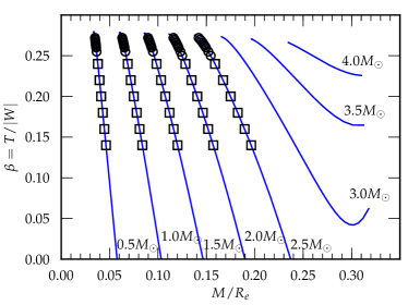
Figure 3: Main features of the five sequences of initial models analyzed in the present work. On the $x$ axis we report the compactness of each stellar model, while its rotation parameter $\beta$ is on the $y$ axis. Squares denote models that are not subject to the bar-mode instability while circles represent the ones that are bar-mode ($m$=$2$) unstable.

Figure 4: Corotation bands for the five sequences of initial models studied in the present work. For each sequence is report the rotation frequency on the axis (where is also reported the mass of the sequence) and on the equator as function of the rotational parameter $\beta$ using continuous-black, doted-blue, dash-dash-doted-green, dash-doted-magenta and dashed-green line for the sequences of baryonic mass $0.5M\odot$, $1.0M\odot$, $1.5M\odot$, $1.0M\odot$ and $2.5M\odot$, respectively. We also shaded, with the corresponding color, the initial part of the corotation bands. For any value of the frequency of a mode between these two lines there is exactly one radius inside the star which is co-rotating with the mode.

An important issue related to the use of polytropic EOS in the construction of the initial models is that their properties are fixed in terms of physical scales determined by the value of the polytropic constant $K$ that can always be set to $1$ by changing the measure units. The assertion that we are generating a model with a giving baryonic mass $M_{0}$ is therefore related to the actual value chosen for $K$. Indeed, in order to claim that the threshold for the instability depends on the stiffness of the EOS, we need to eliminate the dependencies on the dimensional scales and then on the chosen value of the polytropic constant $K$. An efficient way to do that is to extrapolate the result for $M_{0}\rightarrow 0$, which corresponds to the Newtonian limit, where the general relativistic effects can be neglected. Indeed, using the same procedure followed in Manca et al. (2007), we chose five sequences of constant rest-mass density models, namely with $M=(0.5,1.0,1.5,2.0,2.5)\,M_{\odot}$. Again in analogy with Manca et al. (2007), we use a rotational profile with $\hat{A}=1.0$ for all models. We restrict the values of the instability parameter $\beta$ to the range between $0.140$ and $0.272$ and we leave the analysis of models with lower values to future work. The positions of all the simulated models in terms of their compactness $M/R_{e}$, i.e. the ratio between the gravitational mass $M$ and the equatorial radius $R_{e}$, and the rotational parameter $\beta$ are reported in Fig. 3. Since the models are differentially rotating, Fig. 4 shows the corotation bands for the five sequences of models we analyzed.

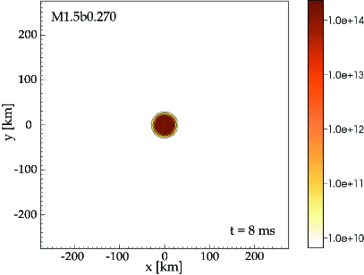
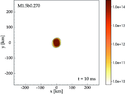
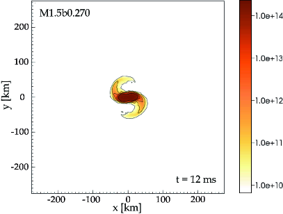
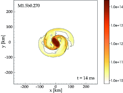
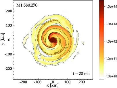
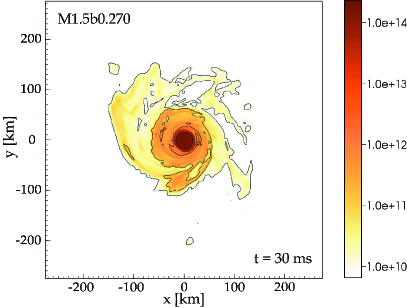
Figure 5: Snapshots of the rest-mass density $\rho$ in the $(x,y)$ plane for M1.5b0.270 at different stage of the evolution, namely $t$=8 and 10 ms (top row), $t$=12 and 14 ms (central row) and $t$=20 and 30 ms (bottom row). The color code is defined in terms of g/cm³.

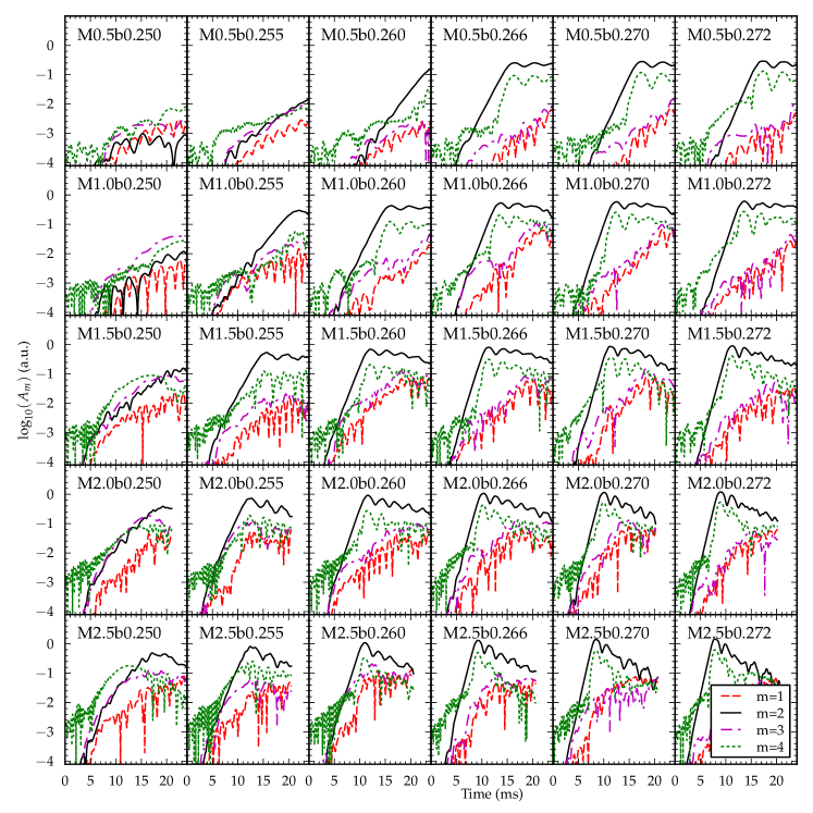
Figure 6: Mode dynamics for selected evolved models that are characterized by a value of the instability parameter $\beta$ between 0.250 and 0.272. All models with $\beta\geq 0.255$ show the typical dynamics one would expect when the dynamical $m=2$ bar mode instability is the dominating phenomenon.

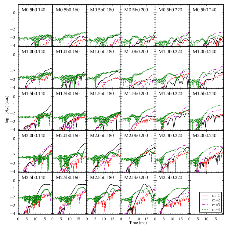
Figure 7: The same as Fig. 6 but for models that are characterized by a value of the $\beta$ parameter in the range $0.14\leq\beta\leq 0.24$.

II.2 Numerical setup and evolution method

The main core of the code used for this work is the Einstein Toolkit Löffler et al. (2012); EinsteinToolkit , which is a free, publicly available, community-driven general relativistic (GR) code, capable of performing numerical relativity simulations that include realistic physical treatments of matter, electromagnetic fields Mösta et al. (2014), and gravity.

The Einstein Toolkit is built upon several open-source components that are widely used throughout the numerical relativity community. Among all of them, only the ones used in this work are mentioned below.

Most components are part of the final evolution code, while others help managing the components Seidel et al. (2010); Allen et al. (2010), building the code and submitting the simulations on supercomputers Thomas and Schnetter (2010); SimFactory , or providing remote debuggers Korobkin et al. (2011) and post-processing and visualization tools for VisIt Childs et al. (2005).

Many components of the Einstein Toolkit use the Cactus Computational Toolkit Cactus developers ; Goodale et al. (2003); Allen et al. (2011), a software framework for high-performance computing (HPC). Cactus simplifies designing codes in a modular (“component-based”) manner, and many existing Cactus modules provide infrastructure facilities or basic numerical algorithms such as coordinates, boundary conditions, interpolators, reduction operators, or efficient I/O in different data formats.

Many of the details of the Einstein Toolkit may be found in Löffler et al. (2012), which describes the routines used to provide the supporting computational infrastructure for grid setup and parallelization, constructing initial data, evolving dynamical GRHD configurations, and analyzing the resulting data describing the properties of the objects being simulated as well as their gravitational wave signatures. The option to evolve magnetic fields, as described in Mösta et al. (2014), is not used here: magnetic fields are not considered in this work. In the following, we only mention or briefly describe the specific methods used for this work together with the chosen, relevant parameters. For details the reader is referred especially to Löffler et al. (2012).

Within this study, the adaptive mesh refinement (AMR) methods implemented by Carpet Schnetter et al. (2004, 2006); Carpet have been used. Carpet supports Berger-Oliger style (“block-structured”) AMR Berger and Oliger (1984) with sub-cycling in time as well as certain additional features commonly used in numerical relativity (see Schnetter et al. (2004) for details). Carpet supports both vertex-centered and cell-centered AMR, but only vertex-centered grids have been used here.

Hydrodynamic evolution techniques are provided in the Einstein Toolkit by the GRHydro package Baiotti et al. (2005); Hawke et al. (2005). The code is designed to be modular, interacting with the vacuum metric evolution only by contributions to the stress-energy tensor and by the local values of the metric components and extrinsic curvature, as we discuss in detail below. It uses a high-resolution shock capturing finite-volume scheme.

The evolution of the spacetime metric in the Einstein Toolkit is handled by the McLachlan package McLachlan . This code is auto-generated by Mathematica using Kranc Husa et al. (2006); Lechner et al. (2004); Kranc , implementing the Einstein equations via a $3+1$-dimensional split using the BSSN formalism Nakamura et al. (1987); Shibata and Nakamura (1995); Baumgarte and Shapiro (1998); Alcubierre et al. (2000, 2003).

The BSSN equations are finite-differenced at a user-specified order of accuracy, and coupling to hydrodynamic variables is included via the stress-energy tensor. The time integration and coupling with curvature are carried out with the Method of Lines (MoL) Hyman (1976), implemented in the MoL package. Within this paper a fourth-order Runge-Kutta Runge (1895); Kutta (1901) method was used, and Kreiss-Oliger dissipation was applied to the evolved quantities of the curvature evolution to damp high-frequency noise.

We use fourth-order difference stencils for the curvature evolution, and $1+\log$ Alcubierre et al. (2003) slicing

$$\partial_{t}\alpha=-2\alpha K,$$ (15)

and $\Gamma$-driver shift condition Alcubierre et al. (2003),

$$\partial_{t}\beta^{i} =\frac{3}{4}B^{i}$$ (16)

$$\partial_{t}B^{i} =\partial_{t}\hat{\Gamma}^{i}-\frac{1}{2}B^{i},$$ (17)

with $K$, $\hat{\Gamma}^{i}$, $\alpha$ and $\beta^{i}$ being the trace of the extrinsic curvature, the conformal connection functions, the lapse factor and the shift, respectively. During time evolution, a Sommerfeld-type radiative boundary condition is applied to all components of the evolved BSSN variables as described in Alcubierre et al. (2000).

All presented results use the Marquina Riemann solver Donat and Marquina (1996); Aloy et al. (1999) and PPM (the piecewise parabolic reconstruction method) Colella and Woodward (1984). An artificial low-density atmosphere with $\rho_{\text{atm}}=10^{-10}$ is used, with a threshold of $\rho_{\text{atm\_reset}}=10^{-7}$ below which regions are reset to atmosphere. Hydrodynamical quantities are set to atmosphere at the outer boundary.

All presented evolutions use a mirror symmetry across the $(x,y)$ plane, consistent with the symmetry of the problem, which reduces the computational cost by a factor of $2$. In addition, one has the possibility to reduce the computational cost by an additional factor of $2$, imposing a rotational $\pi$-symmetry that corresponds to the assumption that the configuration is the same if one applies a rotation of an angle $\pi$ around the $z$-axis. However, in contrast to the mirror symmetry, the $\pi$-symmetry needs to be justified, because previous results De Pietri et al. (2007); Baiotti et al. (2007); Manca et al. (2007) showed that introducing this numerical symmetry by construction prevents odd modes to grow, something that does in fact happen when $\pi$-symmetry is not imposed. Indeed, since we are also interested to investigate whether odd modes play any role, we present here only results obtained by not imposing $\pi$-symmetry and thus we have not taken advance of the 2-fold speedup that would have allowed. Please note that results using $\pi$-symmetry were presented in Löffler et al. (2013) but they related only to the initial stage of the evolution of the dynamical bar-mode in the unstable region (see SubSec. III.3) and the results obtained there have been validated only by the present work.

III Results

As discussed in Sect. I and II, the main goal of the present work is to study the matter instability that may develop in the case of rapidly differentially rotating relativistic star models, using a configuration as close as possible to the realistic case. The other important requirement we need to fulfill is that our study has to be computationally feasible. To achieve this goal, we need to evolve the largest number of models using the available amount of computational resources in the most efficient way. In selecting a numerical setting we can play with many parameters, namely: the location of the outer boundary, the number of refinement levels, the size and resolution of the finest grid and the symmetries to be imposed on the dynamics. All the simulations in the present work are performed using the same setting for the computational domain. More precisely, we use three box-in-box (covering the half space with $z\geq 0$) refinement levels, with boundaries at distances of $L=42,84,168$ from the origin of the coordinate system and grid spacings $dx,2\,dx,4\,dx$, respectively, where we set $dx=0.5$ (that correspond to a resolution $dx\simeq 0.738$ km) unless otherwise noted, corresponding to a hierarchy of three computational grids, each one of size $169\times 169\times 85$ points plus ghost and buffer zones.

We have chosen to use this conservative domain, large enough to capture the whole global dynamics of a bar-mode instability, in order to exclude any influence of the computational setup on observed differences between models. The actual size of the finest grid and the computational set up is determined by the most demanding models. Fig. 5 shows a few snapshots for the evolution of the rest-mass density $\rho$ at different times for a representative model, namely M1.5b0.270 which is characterized by $\beta=0.270$ and $M_{0}=1.5\,M_{\odot}$. This is indeed the typical evolution one would expect for a stellar model which is unstable against the dynamical bar-mode instability.

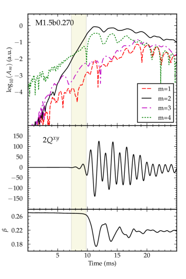
Figure 8: Main features of the dynamics of a representative example of an evolved stellar model that is unstable against the bar-mode instability, namely M1.5b0.270. In particular, we show the time evolution of the power of the cylindrical $m=1,\,2,\,3,\,4$ modes of the matter density (upper panel), the time evolution of the $xy$ component of the quadrupole moment of the conserved density $Q^{xy}$, defined in Eq. (18) (center panel), and the time evolution of the rotational parameter $\beta=T/|W|$. In the shaded region, corresponding to $7$ ms < $t$ < $10$ ms, there is a clear exponential growth of the $m=2$ azimuthal matter mode that later reaches a saturation at $t\approx 12$ ms. Eventually, the model seems to settle down around a new (less differentially rotating) configuration after $t\approx 20$ ms.

III.1 Analysis Methods

In order to compute the growth time of the instability, $\tau_{2}$, we use the quadrupole moments of the matter distribution $Q^{ij}$, computed in terms of the conserved density $D$ as

$$Q^{ij}=\int\!d^{3}\!x\;D\;x^{i}x^{j}\ .$$ (18)

In particular, we perform a nonlinear least-square fit of $Q^{xy}$ (the star spin axis is aligned in the $z$-direction), using the trial function

$$Q^{xy}(t)=Q^{xy}_{0}\mathrm{e}^{\frac{t}{\tau_{2}}}\cos(2\pi f_{2}t+\phi_{0})\,.$$ (19)

Using this trial function, we can extract the growth time $\tau_{2}$ and the frequency $f_{2}$ for the unstable $m=2$ modes. We also define the modulus $Q(t)$ as

$$Q\equiv\frac{1}{2}\sqrt{(2Q^{xy})^{2}+(Q^{xx}-Q^{yy})^{2}}\,,$$ (20)

and the distortion parameter $\eta(t)$ as

$$\eta\equiv\frac{2Q}{(Q^{xx}+Q^{yy})}\,.$$ (21)

Finally, we decompose the rest-mass density into its spatial rotating modes $P_{m}(t)$

$$P_{m}\equiv\int\mathrm{d}^{3}x\,\rho\mathrm{e}^{\mathrm{i}m\phi}$$ (22)

and the “amplitude” and “phase” of the $m$-th mode are defined as

$$A_{m}=|P_{m}|\,\quad\,\text{and}\,\quad\,\phi_{m}\equiv arg(P_{m})\,.$$ (23)

Despite their denomination, the amplitudes defined in Eq. (23) do not correspond to proper eigenmodes of oscillation of the star but to global characteristics that are selected in terms of their spatial azimuthal shape. All Eqs. (19)-(23) are expressed in terms of the coordinate time $t$, and therefore they are not gauge invariant. However, the length scale of variation of the lapse function at any given time is always small when compared to the stellar radius, ensuring that events close in coordinate time are also close in proper time.

III.2 General features of the evolution above the threshold for the onset of the bar-mode instability

The above mentioned general features of the evolution are common to all the modes that show the expected dynamics in presence of the well studied bar-mode $m=2$ instability. In Fig. 6 the “mode-dynamics” of most of the studied models having $\beta\geq 0.25$ are shown. For all these models (except for M0.5b0.250 and M1.0b0.250) it is indeed possible to extract the main features of the $m=2$ mode using the procedure detailed in Eq. (19). Fig. 8 shows the time evolution of some quantities that characterize the behavior of model M1.5b0.270, for which also some snapshots were shown in Fig. 5. We decided to quantify the properties of the bar-mode instability by means of a nonlinear fit, using the trial dependence of Eq. (19) on a time interval where the distortion parameter $\eta$ defined in Eq. (21) is between $1\%$ and $30\%$ of its maximum value. The shaded region in Fig. 8 corresponds exactly to the region we selected for the fit according to this criterion.

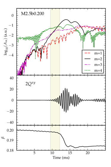
Figure 9: The same as Fig. 6 but for model M2.5b0.200, that shows the presence of a $m=2$ shear instability at a low value of $\beta$. The dynamics enclosed in the shaded region has been selected to compute the characteristic frequency and growth time of the $m=2$ instability, that turned out to be $f_{2}=1.943$ kHz and $\tau_{2}=1.02$ ms respectively.

The results of all these fits are collected in Tab. 1, where we report for each model the maximum value assumed by the distortion parameter $\max(\eta)$, the time interval $[t_{i},t_{f}]$ selected for the fit, the value $\beta(t_{i})$ corresponding to the value of the instability parameter $\beta$ at the beginning of the fit interval and $\tau_{2}$ and $f_{2}$, the growth time and frequency that characterize the $m=2$ bar-mode instability, respectively.

Figure 10: Here we show the frequency of the corotation band multiplied by 2 (shaded region) and the measured values for the coordinate frequency of the observed $m=2$ modes (circles) for all the models belonging to the sequence with baryon mass $M_{0}=2.5M_{\odot}$.

III.3 General features of the evolution below the threshold for the onset of the bar-mode instability

The situation is more complicated for initial models characterized by lower values of the $\beta$ parameter, i.e. $\beta<0.245$. For these models (see Fig. 7) one can observe there is an indication that instabilities are present. For example, models like M0.5b0.200, M0.5b0.220, M0.5b0.240 and M2.0b0.200, M2.0b0.220, M2.0b0.240 show the possible presence of a three-arms, $m=3$, unstable mode. Other models, e.g. M2.0b0.140, seem to show a competition between two different unstable modes, namely the $m=2$ mode and the $m=3$ mode.

Other models show the presence of $m=2$ unstable modes. We use as a practical criteria to select such models the fact that they have a maximal distortion parameter $\eta$ greater than $10\%$, i.e. $\max(\eta)>0.10$. The simulated models that fulfill this criteria are: models M1.0b0.140 and M1.0b0.160, belonging to the sequence with $M_{0}=1.0$; model M1.5b0.140 for $M_{0}=1.5$; models M2.0b0.140, M2.0b0.160, M2.0b0.180 for $M_{0}=2.0$ and, finally, models M2.5b0.140, M2.5b0.160, M2.5b0.180, M2.5b0.200 and M2.5b0.220 for the $M_{0}=2.5$ sequence. For example, in the case of model M2.5b0.200 (see Fig. 9) we can observe an exponential growth, with a frequency $f_{2}=1.95$ kHz and a growth time $\tau_{2}\simeq 1$, of the $m=2$ mode developing and eventually saturating at about 12 ms, when the model settles down to a new equilibrium configuration corresponding to a lower value of the rotational parameter $\beta$ and a different differential rotation profile. Indeed, the frequency of all these $m=2$ modes are inside the corotation band (see Fig. 10) and should be classified as shear instabilities, of the same type of those observed in Corvino et al. (2010).

The same check has been performed for all unstable modes (both those with $m=2$ and those with $m=3$) that are indeed shear instabilities. In particular, for the $m=2$ of the models with $M_{0}=2.5$ below the threshold for the onset of the classical dynamical bar-mode instability, in Fig. 10 it is shown that the frequency $f_{2}$ of the unstable model are within the corotation band.

model	$\max(\eta)$	$t_{i}$	$t_{f}$	$\beta(t_{i})$	$\tau_{2}$(ms)	$f_{2}$(kHz)
M0.5b0.255	0.178	13.2	26.2	0.2527	3.913	0.527
M0.5b0.260	0.404	14.8	21.3	0.2573	1.899	0.515
M0.5b0.262	0.473	12.3	17.7	0.2597	1.604	0.512
M0.5b0.264	0.515	13.4	18.4	0.2612	1.474	0.508
M0.5b0.266	0.578	9.2	13.7	0.2639	1.307	0.505
M0.5b0.268	0.615	11.2	15.4	0.2656	1.223	0.502
M0.5b0.270	0.664	11.1	15.0	0.2674	1.150	0.496
M0.5b0.272	0.713	11.3	15.0	0.2695	1.085	0.493
M1.0b0.255	0.475	11.2	18.0	0.2532	1.959	0.685
M1.0b0.260	0.702	9.2	13.5	0.2584	1.256	0.673
M1.0b0.262	0.776	8.4	12.3	0.2605	1.152	0.668
M1.0b0.264	0.836	8.6	12.2	0.2623	1.037	0.663
M1.0b0.266	0.893	8.3	11.6	0.2645	0.964	0.658
M1.0b0.268	0.936	8.3	11.5	0.2665	0.908	0.652
M1.0b0.270	0.992	7.5	10.5	0.2685	0.863	0.646
M1.0b0.272	1.021	8.9	11.8	0.2698	0.826	0.639
M1.5b0.250	0.180	6.7	17.1	0.2494	3.260	0.860
M1.5b0.255	0.658	8.1	12.8	0.2537	1.380	0.835
M1.5b0.260	0.864	6.7	10.1	0.2589	0.976	0.816
M1.5b0.262	0.908	8.5	11.7	0.2604	0.949	0.809
M1.5b0.264	0.974	7.5	10.4	0.2624	0.853	0.802
M1.5b0.266	1.043	6.9	9.6	0.2648	0.789	0.796
M1.5b0.268	1.086	7.6	10.2	0.2666	0.747	0.787
M1.5b0.270	1.123	7.3	9.8	0.2683	0.721	0.778
M1.5b0.272	1.175	7.3	9.7	0.2699	0.696	0.770
M2.0b0.250	0.362	7.6	14.8	0.2486	2.203	1.023
M2.0b0.255	0.749	6.4	10.2	0.2536	1.140	0.988
M2.0b0.260	0.917	6.9	9.8	0.2582	0.849	0.969
M2.0b0.262	0.995	7.3	10.0	0.2604	0.806	0.953
M2.0b0.264	1.059	7.2	9.7	0.2628	0.731	0.942
M2.0b0.266	1.121	6.5	8.8	0.2647	0.687	0.934
M2.0b0.268	1.155	6.6	8.9	0.2667	0.650	0.923
M2.0b0.270	1.203	6.5	8.6	0.2686	0.626	0.912
M2.0b0.272	1.245	5.6	7.6	0.2707	0.596	0.900
M2.5b0.250	0.372	7.1	13.7	0.2480	1.843	1.195
M2.5b0.255	0.684	7.0	10.6	0.2530	1.042	1.158
M2.5b0.260	0.922	6.7	9.4	0.2583	0.798	1.121
M2.5b0.262	1.010	5.7	8.1	0.2608	0.711	1.112
M2.5b0.264	1.073	5.6	7.9	0.2625	0.667	1.097
M2.5b0.266	1.118	5.8	7.9	0.2646	0.627	1.085
M2.5b0.268	1.173	5.5	7.5	0.2666	0.586	1.072
M2.5b0.270	1.221	5.3	7.3	0.2688	0.565	1.051
M2.5b0.272	1.261	4.9	6.8	0.2710	0.541	1.033

Table 1: Results for the growth time $\tau_{2}$ and the frequency $f_{2}$ of the bar-mode for all the models that show the presence of the bar-mode instability. The values are obtained from simulations which employ a spatial resolution $dx=0.5$ for the finest grid.

III.4 Effects of the compactness on the threshold for the onset of the bar-mode instability

We have chosen to investigate the effect of the compactness on the classical bar-mode instability, at fixed stiffness, following the same procedure as in Manca et al. (2007). We determined the critical value of the instability parameter $\beta$ for the onset of the instability by simulating five sequences of initial models having the same value of $M_{0}$ but different values of $\beta$. For these simulations we decided to employ the same resolution $dx=0.5$ on the finest grid for all the simulations. This choice was mainly motivated by the necessity to keep the computational cost under reasonable limits.

We now restrict our analysis to the models for which we observed the maximum value of the distortion parameter $\eta$ to be greater than $0.10$. For these models, we explicitly checked that the reported unstable modes correspond to the classical bar-mode instability and not to a shear-instability by checking that the frequency of the mode divided by two is not in the corotation band of the model (see Fig. 4). This is effectively true for all the reported models, except for M2.5b0.250, M2.5b0.255 and M2.5b0.260, which are just marginally (at the lower boundary) on the corotation band (see Fig. 10).

Figure 11: Critical diagram relating the growth time $\tau_{2}$ of each bar-mode unstable model to the value of the instability parameter $\beta$. Triangles represent the values corresponding to all the models listed in Tab. 1. More precisely, the quantity on the $x$-axis is actually expressed in terms of $1/\tau_{2}^{2}$, in order to highlight the very good fit, while the quantity on the $y$ axis is the value of $\beta$ at the beginning of the time interval chosen for performing the fit of $m=2$ mode growth, reported in Tab. 1 as $\beta(t_{i})$. For all the five constant rest-mass sequences considered we also report, with open circles, the extrapolated value $\beta_{c}$ and the fitted straight lines with Eqs. (26).

Figure 12: The open circles are the same as in Fig. 11, but here they are shown as a function of the baryonic mass $M_{0}$. The filled circle, on the other hand, marks the extrapolation for zero rest-mass, representing the limit of Newtonian gravity (or zero compactness). The result of this extrapolation is reported in Eq. (27).

We have performed a fit for the growth time $\tau_{2}$ of the bar mode as a function of the instability parameter $\beta$ for five sequences of models with constant rest-mass ranging from 0.5 $M_{\odot}$ to 2.5 $M_{\odot}$, as shown in Fig. 11. Let us estimate the threshold for the onset of the instability using the extrapolation technique used in Manca et al. (2007) where we assume, in analogy with what expected in the Newtonian case, that the main dependence of the frequency of the mode on $\beta$ is of the type

$$\sigma(\beta)=\Omega(\beta)\pm\sqrt{F(\beta)}\,,$$ (24)

where

$$\frac{1}{(\tau_{2}(\beta))^{2}}=F(\beta)\simeq A(\beta_{c}-\beta)\,.$$ (25)

Under this assumption, we find the following values for the critical fit of the growth times:

$$0.5M_{\odot} : 1/{(\tau_{2})^{2}} =6.85(4) \!\!\!\!\times\,(0.2512(2)-\beta)$$ (26)

$$1.0M_{\odot} : 1/{(\tau_{2})^{2}} =8.46(20) \!\!\!\!\times\,(0.2497(7)-\beta)$$

$$1.5M_{\odot} : 1/{(\tau_{2})^{2}} =9.83(24) \!\!\!\!\times\,(0.2483(7)-\beta)$$

$$2.0M_{\odot} : 1/{(\tau_{2})^{2}} =10.86(23) \!\!\!\!\times\,(0.2469(7)-\beta)$$

$$2.5M_{\odot} : 1/{(\tau_{2})^{2}} =11.80(35) \!\!\!\!\times\,(0.2463(7)-\beta)$$

The results obtained so far cannot be directly compared with those obtained in Manca et al. (2007) to infer the effects of considering a stiffer EOS. The main issue is that when considering a polytropic EOS, one can change the units of measurement in such a way that the value of the polytropic constant $K$ is $1$. This means that by changing this value one effectively changes the mass scale and, in turn, the mass of the considered stellar model. Indeed, the assertion that for a star with mass $M_{0}=1.0M_{\odot}$ the threshold for the onset of the bar-mode instability is reduced to $0.2497(7)$ for $\Gamma=2.75$ from the higher value of $0.2598(8)$ for $\Gamma=2.0$ is susceptible to the choice of the mass scale determined by the choice of the values of the polytropic constants. This dependence from the choice of the mass scale can be eliminated by going to the zero-mass limit that corresponds to performing an extrapolation to the Newtonian limit of the results. This can be achieved by a linear fit of the reported values for the critical $\beta_{c}$ for the onset of the classical bar-mode instability of Eqs. (26) as a function of the baryonic rest-mass (see Fig. 12). The overall result for this fit leads to the following expression for the critical $\beta_{c}$ as a function of the the total baryonic mass $M_{0}$:

$$\beta_{c}(M) =0.2527(4)-0.0027(5)M_{0}\,.$$ (27)

The extrapolated value for $\beta_{c}$ in the limit of zero baryonic mass for the relativistic stellar models then leads to $\beta_{c}^{N}=0.2527(4)$ for $\Gamma=2.75$, which can now be directly compared to the one obtained in Manca et al. (2007), i.e. $\beta_{c}^{N}=0.266(1)$ for $\Gamma=2.0$. A further consistency check that the extrapolated threshold actually corresponds to the Newtonian value can be found in the literature for the case of $\Gamma=2$. In fact, of the four models discussed in Saijo and Kojima (2008); Kojima and Saijo (2008), the one characterized by $\beta=0.281,\,0.277,\,0.268$ are unstable, while the one characterized by $\beta=0.256$ is stable.

This shows that the threshold for the onset of the dynamical bar-mode instability is significantly but not greatly reduced by an increase in the stiffness of the EOS, induced by a change of $\Gamma$ from 2 to 2.75. Unfortunately, this threshold is very close to the maximum possible value for $\beta$ that can be sustained by a realistic EOS like the one obtained from the SLy prescription. As it was shown in Corvino et al. (2010), there are very few relativistic models with $\hat{A}=1$ that can be generated with a value of $\beta$ above the threshold for the dynamical bar-mode instability even if we consider the effect of using a stiffer EOS.

III.5 Resolution

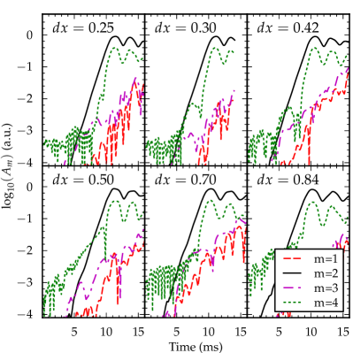
Figure 13: Evolution of M1.5b0.270 for different values of the resolution on the finest grid. Note that the total computational cost of the simulation at resolution $dx=0.25$ is 16 times greater than a simulation at dx=0.5.

In order to asses the correctness of the extracted value of $\beta^{N}_{c}$ one has to check how the result depends on the actual resolution used. To perform this check we have evolved a typical model (M1.5b0.270) characterized by the same value of the initial baryonic mass $M_{0}=1.5M_{\odot}$ and a value of the initial rotation parameter $\beta=0.270$ using different grid resolutions, namely varying the grid spacing in the range from $dx=0.25$ to $dx=0.84$ in dimensionless units where $G=c=1$. That corresponds to resolutions varying between $dx=0.369$ km and $dx=1.240$ km. The results of the mode evolutions we have obtained are shown in Fig. 13. The mode dynamics we obtained show that the overall picture of the dynamics does not change.

However the actual results of the fits, as expected, show a dependence on the used resolution. In Table 2 we report: the resolution used, the maximum value reached by the distortion parameter $\eta$, the time $t_{i}$ and $t_{f}$ for which the distortion parameter has a value between the 1% and the 30% of the maximum, the value of the rotational parameter at the time $t_{i}$ and the fitted values for the growth time and frequency of the unstable bar-mode.

resolution	max($\eta$)	$t_{i}$	$t_{f}$	$\beta(t_{i})$	$\tau_{2}$(ms)	$f_{2}$(kHz)
dx=0.25 (0.369 km)	1.164	7.4	9.8	0.2697	0.692	0.783
dx=0.30 (0.443 km)	1.154	7.1	9.5	0.2695	0.693	0.784
dx=0.42 (0.620 km)	1.147	6.6	9.0	0.2692	0.706	0.780
dx=0.50 (0.738 km)	1.123	7.3	9.8	0.2683	0.721	0.778
dx=0.70 (1.034 km)	1.111	6.1	8.6	0.2675	0.742	0.770
dx=0.84 (1.240 km)	1.049	5.9	8.5	0.2658	0.768	0.771

Table 2: Results of the fitw of the grow times $\tau_{2}$ as a function of the resolution for model M1.5b0.270.

Figure 14: Here we show the time evolution of the $\beta$ parameter for different values of the employed resolution. The filled dots mark the time at which the values $\beta(t_{i})$, used in the fits are evaluated.

Figure 15: The filled circles represent the values of $\beta$ at the time when the distortion parameter $\eta$ reaches 1% of its maximum value, as a function of the inverse of the square of the growth time, for model M1.5b0.270 at different resolutions for the finest grid. The straight line represents the result of the fit (as a function of $\beta$) for the whole sequence of models at fixed value of the conserved baryonic mass $M_{0}=1.5M_{\odot}$ and at resolution $dx=0.50$. The open triangles represent the values of two different models among them.

While the overall dynamics is very similar for all resolutions, there is a consistent shift of the value of the $\beta$ parameter at the beginning of the development of the instability $\beta_{i}$ and of the value of the fitted growth time $\tau_{2}$ with increasing resolution. More precisely, the analysis of the initial stage of the evolution shows (see Fig. 14) that there is indeed a drift (decrease) of the value of $\beta$ and, consequently, the fit of $\tau_{2}$ is sensible to the value used for a given resolution. This can, at least partially, be explained to be due to the fact that by the time the amplitude of the mode reaches the fit-window, the evolution does not correspond any longer to the original model but it is closer to a new equilibrium model (through an adiabatic drift), characterized by a different value of the rotational parameter $\beta$. The overall conclusion is that one has to be careful when associating the fitted value for the growth time of the instability to the initial value of the rotational parameter $\beta$. In fact, as it can be seen in Fig. 14, there is a small shift (of as much as 2% for the lowest resolution) of the value of $\beta$ from the start of the simulation up to the time at which the instability is detected ($\beta_{i}=\beta(t_{i})$). Using this fact, we now report in Fig. 15 the growth-time and the $\beta$ at the beginning of the instability for each resolution and the critical fit of Eq. (26) for $M_{0}=1.5M_{\odot}$. That shows we have convergence in the determination of the parameter of the classical bar-mode instability above the threshold, if we use the value $\beta_{i}$ to perform the extrapolations.

While these results show that the used resolution is enough to explore the dynamical bar-mode instability, we cannot draw such conclusion on the parameter of the observed shear-instability at lower $\beta$. Despite that we did observe that such instabilities are present, the resolution used here is not sufficient to draw conclusions about their numerical values. We note that we found candidates of $m=2$ shear instability when examining several models in different resolutions, but the instability dynamics cannot be clearly singled out with respect to other instabilities that seem to be present. One example is given in Fig. 16, which shows that the interplay on the growth of various modes shows some dependency on the resolution. Such dependency was not observed in the cases where the classical dynamical bar-mode instability is present and it is by far the fastest growing mode.

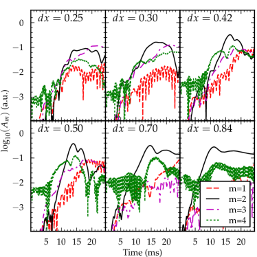
Figure 16: Resolution’s effect on the mode dynamics for model M2.5b0.200. In the case of models below the threshold the interplay of modes with different shapes does not show a clear convergent behavior on the dynamics.

This shows that for these values of $\beta$ the used resolution on the finer grid of $dx=0.50$ is not enough to determine the dynamics of the shear instability. This initial analysis show that a resolution of, at least, $dx=0.25$ is needed. Moreover, in this case, the use of the numerical discretization error to triggering the fastest growing mode does not seem to be the best strategy to study shear instabilities when a competition between different $m$ modes (like $m=2$ and $m=3$) is present. We will leave a detailed study of the low-$beta$ instabilities to a future work.

IV Conclusions

We have presented a study of the dynamical bar-mode instability in differentially rotating NSs in full General Relativity for a wide and systematic range of values of the rotational parameter $\beta$ and the conserved baryonic mass $M_{0}$, using a polytropic/ideal-fluid EOS characterized by a value of the adiabatic index $\Gamma=2.75$, which allows us to resemble the properties of a realistic EOS. In particular, we have evolved a large number of NS models belonging to five different sequences with a constant rest-mass ranging from $0.5$ to $2.5\,M_{\odot}$, with a fixed degree of differential rotation ($\hat{A}=1$) and with many different values of $\beta$ in the range $[0.140,0.272]$.

For all the models with a sufficiently high initial value of $\beta$ we observe the expected exponential growth of the $m=2$ mode which is characteristic of the development of the dynamical bar-mode instability. We compute the growth time $\tau_{2}$ for each of these bar-mode unstable models by performing a nonlinear least-square fit using a trial function for the quadrupole moment of the matter distribution. The growth time clearly depends on both the rest-mass and the rotation and in particular we find that the relation between the instability parameter $\beta$ and the inverse square of $\tau_{2}$, for each sequence of constant rest-mass, is linear.

This allows us to extrapolate the threshold value $\beta_{c}$ for each sequence corresponding to the growth time going to infinity, using the same procedure already employed in Manca et al. (2007). Once the five values of $\beta_{c}$ have been computed, we are able to extrapolate the critical value of the instability parameter for the Newtonian limit, which is found to be $\beta_{c}^{N}|_{\Gamma=2.75}=0.2527$. This value can be directly compared with the one found in Manca et al. (2007) for the “standard” $\Gamma=2$ case, which is $\beta_{c}^{N}|_{\Gamma=2}=0.266$.

Our results suggest that, even if one can now consider just two values for the adiabatic index, namely the values $\Gamma=2.75$, considered in the present work, and $\Gamma=2$, considered in Baiotti et al. (2007); Manca et al. (2007), the use of a stiffer, more realistic EOS should be expected to have the effect of reducing the threshold for the onset of the dynamical bar-mode instability. Unfortunately, the actual reduction of the threshold $\beta_{c}$ is just of the order of $5\%$, and indeed this reduction does not lead to a significantly higher probability for it to occur in real astrophysical scenarios.

We also evolved many models belonging to the same five sequences but having lower values of the instability parameter $\beta$. We find that many of them show the growth of one or more modes even though their initial value of $\beta$ is below the threshold for the onset of the dynamical bar-mode instability. The modes that show a growth are mainly $m=2$ and the $m=3$. We compute the frequencies of these growing modes and compare them with the corotation band for their progenitor models, finding that all those frequencies are within this band. We can conclude that such instabilities have to be defined as shear instabilities, as the ones that were already observed in Corvino et al. (2010).

Unfortunately, we are not able to measure their growth time, since their dynamics change significantly by changing the resolution of the simulations. In fact, while at a coarse resolution we usually observe only one mode growing exponentially, when improving the resolution other modes develop as well and the interplay between these prevent a clear exponential growth of only one mode which could dominate the evolution.

In order to make a quantitative assessment about this phenomenon, either much higher resolution has to be used to see if one of the modes is able to dominate, or seed perturbations have to be introduced with the aim of selecting only a particular mode at a time. We leave this treatment to futures studies.