Infrared Gluon Resummation and pp total cross-sections

Abstract:

We address here the problem of describing both the total & the elastic proton-proton cross-section, through the four outstanding features of hadron scattering: (i) the optical point; (ii) the forward peak, (iii) the dip & (iv) the subsequent descent at larger momentum transfers. These issues are discussed through an eikonal model for the elastic amplitude where the matter distribution in impact parameter space is given by resummed soft gluons down into the infrared (IR) region. The asymptotic growth of the total cross-section is obtained in a mini-jet model and the taming (saturation) at high energies is related to confinement realized here through an IR singular strong coupling constant $\alpha_{s}(Q^{2})$. We present an ansatz that links the IR singularity of $\alpha_{s}(Q^{2})$ to that of asymptotic freedom (AF) (at lowest order). Through this model, we illustrate the problems that arise in a generic one-channel eikonal model employed for a description of the measured differential elastic cross-section at LHC7.

1 Introduction

The momentum transfer ($t$) dependence of the elastic differential cross-section, recently measured by the TOTEM Collaboration [1], can be dissected into the following elemental components:

• the optical point:, i.e. the value at $t=0$ which is proportional to the square of the total cross-section, modulo a small correction due to $\rho(s)^{2}$, where $\rho$ is the ratio of the real to imaginary part of the elastic amplitude at $t=0$,

• the Coulomb region: which carries a $t$-dependence $\sim F_{p}^{4}(t)/|t|^{2}$, through the well-known Rutherford scattering cross section, represents a key piece to determine $\rho(s)$ in the interference region with hadronic amplitude at small $t$.

• the forward peak, i.e. the decrease for small $t$ values is well described by an exponential in $t$, i.e. a gaussian fall off in the Fourier transform space, $\bf b$-space,

• the dip-bump, namely the occurrence of a sharp dip for $t_{D}=-t_{dip}$ with $t_{D}$ an energy dependent value, which can be seen to satisfy a new geometric scaling law, $\tau_{geo}=t_{D}\sqrt{\sigma_{elastic}\sigma_{total}}=constant$ [2],

• the tail, the region after the dip-bump, where the cross-section starts decreasing once more with a behaviour equally well described by an exponential in $t$ or by a power law, i.e. $|t|^{-n}$ with $n\lesssim 8$ [1, 3].

In what follows we shall address the optical point question and the behavior around the dip, including the scaling properties, with a mini-jet model inclusive of IR gluon resummation [4, 5] ( labelled as BN for reasons to be explained ). We shall start with the forward peak, as a way to introduce the BN model as well.

2 The optical point, i.e. the total cross-section

With the notation:

$$\sigma_{total}=4\pi\Im m\mathcal{F}(s,0)$$

$$\frac{d\sigma_{el}}{dt}=\pi|i\Im m\mathcal{F}(s,t)+\Re e\mathcal{F}(s,t)|^{2}$$ (1)

the value of the differential elastic cross-section at the optical point, i.e. at $t=0$, can be written as

$$\frac{d\sigma_{el}}{dt}|_{t=0}=\pi|\Im m\mathcal{F}(s,0)|^{2}(1+\rho(s)^{2})=[\frac{\sigma_{total}^{2}}{16\pi}][1+\rho(s)^{2}]$$ (3)

$$\rho(s)=\frac{\Re e\mathcal{F}(s,0)}{\Im m\mathcal{F}(s,0}$$ (4)

Thus, to reproduce the optical point value, we need a good model for the total cross-section. Let us begin with a simple single-eikonal model, with a purely imaginary amplitude, i.e.,

$$\mathcal{F}(s,t)=i\int[\frac{d^{2}\bf b}{2\pi}]e^{i\bf b\cdot\bf q}[1-e^{-\bar{n}(b,s)/2}]$$ (5)

with $-q^{2}=t$. We have seen [6] that in one channel eikonal models such as the above, the purely imaginary eikonal function corresponds to the average number $\bar{n}$ of independent collisions in impact parameter space. At high energy, such collisions are mostly describable through QCD parton-parton collisions. Postulating factorization between the energy dependence and the impact momentum variable, and an empirical separation between soft and hard, both reasonable approximations at high energy, one can write

$$\bar{n}=\bar{n}_{soft}(b,s)+\bar{n}_{hard}(b,s)$$ (6)

In our mini-jet model [4, 5, 7], we parametrize the low energy behaviour, namely up to $\sqrt{s}\approx 5\ GeV$, while making the hypothesis that the rise is due to QCD processes, namely parton-parton scattering, resulting in so called mini-jets. In such models, one writes:

$$\bar{n}_{soft}(b,s)=A_{soft}(b,s)\sigma_{soft}(s)$$ (7)

$$\bar{n}_{hard}(b,s)=A_{hard}(b,s)\sigma_{mini-jet}(s)$$ (8)

To determine the impact parameter dependence, we apply two different procedures to the soft and to the hard term. Since our aim, at present, is to apply QCD to the rising part of the cross-section, for the soft term our model uses an impact parameter distribution obtained from the convolution of the electromagnetic form factors of the colliding particles. For the hard, mini-jet, term, we introduce the Fourier transform of the Soft Gluon Resummation expression, namely

$$A_{hard}(b,s)\equiv A_{BN}(b,s)=\mathcal{N}e^{-h(b,s)}$$ (9)

$$h(b,s)=\frac{8}{3\pi^{2}}\int_{0}^{qmax}d^{2}{\bf k}_{t}\frac{\alpha_{s}(k_{t}^{2})}{k_{t}^{2}}[1-e^{-i\bf b\cdot\bf k_{t}}]\ln(2q_{max}/k_{t})$$ (10)

where the subscript $BN$ refers to the fact that in this model all values of $k_{t}$ contribute to the integral, just as in the original Bloch and Nordsieck discussion of the infrared divergence in electrodynamics [8]. The upper limit of the single $k_{t}$ integration, is called $q_{max}$ and depends on energy and the specific parametrization of the Parton Density Functions (PDFs) used in the mini jet cross-sections [4, 9]. We have commented about the function $h(b,s)$ in our publications, here we recall our ansatz: when $k_{t}<\Lambda$ we introduce a singular effective quark-gluon coupling, albeit the final expression is integrable, namely

$$\alpha_{s}(k_{t}^{2})\simeq(\frac{k_{t}}{\Lambda})^{-2p},\ \ \ \ k_{t}^{2}<<\Lambda^{2}$$ (11)

with $p<1$ for the integral of Eq.  (10) to exist. In [4] we had made the phenomenological approximation

$$\alpha_{s}(k_{t}^{2})=\frac{p}{b_{0}\ln[1+p(\frac{k_{t}^{2}}{\Lambda^{2}})^{p}]}$$ (12)

$$\alpha_{s}(k_{t}^{2})\to\frac{1}{b_{0}}(\frac{k_{t}}{\Lambda})^{-2p}\ \ \ \ k_{t}^{2}<<\Lambda^{2}$$ (13)

$$\alpha_{s}(k_{t}^{2})\to\alpha_{s}^{AF}(k_{t}^{2})=\frac{1}{b_{0}\ln[\frac{k_{t}^{2}}{\Lambda^{2}}]}\ \ \ \ k_{t}^{2}>>\Lambda^{2}$$ (14)

with $b_{0}=(33-2N_{f})/12\pi$. A simpler and more interesting proposal would be to identify the singularity parameter $p$ with the LO coefficient of the $\beta-$ function, $b_{0}$, through the following simple rewriting of the QCD Asymptotic Freedom expression for $\alpha_{s}$, i.e. since

$$\alpha_{s}^{AF}(Q^{2})=\frac{1}{\ln[(\frac{Q^{2}}{\Lambda^{2}})^{b_{0}}]}$$ (15)

we propose to substitute the above with an effective expression for the strong coupling constant given by

$$\alpha_{s}^{BN}(Q^{2})=\frac{1}{\ln[1+(\frac{Q^{2}}{\Lambda^{2}})^{b_{0}}]}$$ (16)

Just as the empirically proposed expression in Eq. (12), the expression in Eq.(16) can then be used in the entire region of interest for resummation, extended safely down to $k_{t}=0$. The suffix BN is used to indicate precisely this, namely that it can be used down into the infrared region. The advantage of this expression is that it does not require introduction of an extra parameter $p$: the behavior from $Q^{2}=0$ to $Q^{2}\to\infty$ is dictated only by the anomalous dimension factor.

The above proposal will be further elaborated in a separate publication. Here, it suffices to say that the anomalous dimension factor $b_{0}<1$, and thus $\alpha_{s}^{BN}$ satisfies the condition for integrability of our resummation function $h(b,s)$ in Eq. (10). In Fig.  1 we show the behaviour of the proposed expression Eq. (16), for the case $N_{f}=3$, as a function of $Q^{2}/\Lambda^{2}$.

Figure 1: The asymptotic freedom expression for the strong coupling constant and our proposed expression, plotted as a function of $Q^{2}/\Lambda^{2}$, for the case $N_{f}=3$.

Notice however that the numerical results we are presenting, and have presented so far, will still use the empirical expression of Eq.  (12), and that the parameter $p$ has so far been determined on purely phenomenological grounds. As we shall see, values for a good representation of the total cross-section, are such that $p\simeq 0.6\div 0.75$ depending on the PDF’s used, while $b_{0}$ varies between 0.56 and 0.77, for $N_{f}=6,\ 2$, respectively. The ansatz of Eq.(16) is based on the LO expression for $\alpha_{s}$, of course, and a closer correspondence needs further study.

The behavior of Eq. (11) introduces a cut-off in $\bf b$-space [10] such that asymptotically the total cross-section behaves as

$$\sigma_{total}\sim[\epsilon\ln s]^{1/p}$$ (17)

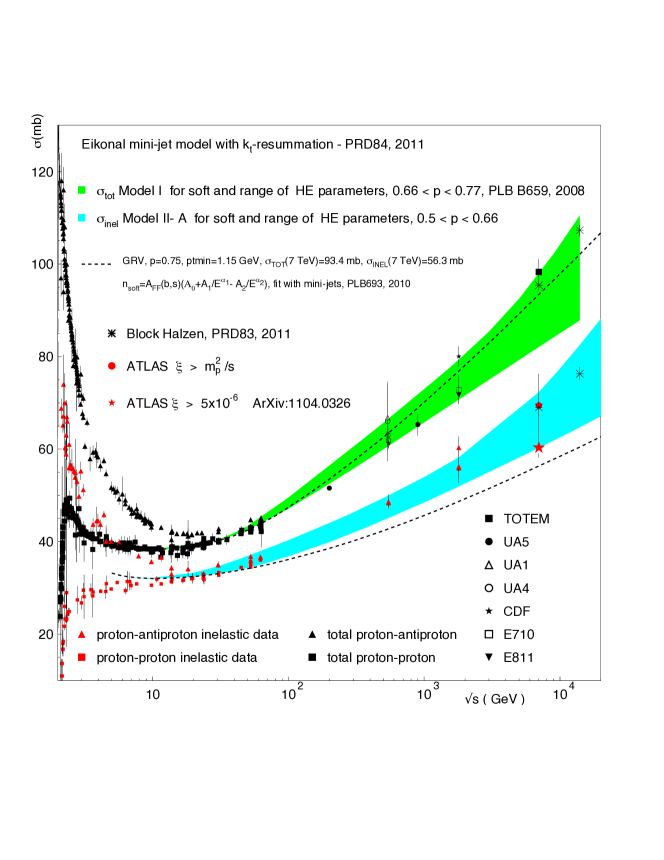
where $\epsilon\simeq 0.3-0.4$ corresponds to the asymptotic behavior of the mini-jet cross-section, i.e. $\sigma_{mini-jet}\sim s^{\epsilon}$ as $\sqrt{s}\rightarrow\infty$. The energy rise predicted by this model depends on a parameter set consisting of the singularity parameter $p$, the minimum mini-jet transverse momentum $p_{tmin}$ needed to avoid the Rutherford singularity in the parton-parton cross-section, and the PDFs, chosen to be at Leading Order (LO) to avoid double counting with soft resummation contributions. Using different PDF sets, GRV [11] and MRST [12], we show in Fig.  2 expectations for both total and inelastic cross-sections from [6].

Figure 2: Total and inelastic pp cross-section using the BN model from [6].

Thus the model is now well defined and can be applied to study the elastic differential cross-section.

3 The elastic, total and differential, cross-section in the BN model

3.1 Total cross-sections, elastic and inelastic

We now apply the mini-jet model with Soft Gluon Resummation (SGR) as described in the first section to study the integrated elastic and differential $pp$ cross-sections. As pointed out in [6], in a one-channel eikonal model, the division between elastic and inelastic contributions is misguided , namely the expressions

$$\sigma_{elastic}=\int d^{2}{\bf b}|1-e^{-\bar{n}(s,b)/2}|^{2}$$ (18)

$$\sigma_{inel}=\int d^{2}{\bf b}[1-e^{-\bar{n}(s,b)}]$$ (19)

$$\sigma_{total}=2\int d^{2}{\bf b}[1-e^{-\bar{n}(s,b)/2}]$$ (20)

do not include all inelastic processes into $\sigma_{inel}$, but only uncorrelated inelastic ones. If one uses the above simple formalism, it follows that diffractive, or correlated processes, are actually counted into $\sigma_{elastic}=\sigma_{total}-\sigma_{inel}$. Two or many-channel formalism and models for the diffractive part of the inelastic cross-section, have been invoked to solve this difficulty. We seek here a different phenomenological way out.

Such a phenomenological way out, barring the introduction of more parameters, is to use different values for the singularity parameter $p$ for the elastic and the total cross-section. For illustration, we can use a representative parameter set such as, for instance, $\{GRV,p_{tmin}=1.15\ GeV\}$. This set allows to describe $\sigma_{total}$ with $p=3/4$, while $\sigma_{elastic}$ can be obtained with a different value: $p=5/6$. Similarly, using for densities the MRST72 set, we find that the elastic cross-section data need a higher p-value than the total cross-section data. Notice that changing the PDFs and/or $p_{tmin}$, which are correlated parameters, will also slightly change the $p$ values, but what matters in the discussion here is that the $p$ value describing $\sigma_{elastic}$ is larger for the elastic cross-section. As long as $\sigma_{elastic}$ is not rising at the same rate as $\sigma_{total}$, namely as long as ${\cal R}_{el}=\sigma_{el}/\sigma_{tot}\neq 1/2$, this is an obvious consequence of Eq. (17), but if the ansatz of Eq.  (16) is correct, this matches with its naive understanding: in the elastic cross-section only two flavors are present, and $p=b_{0}(N_{f}=2)=0.77$, while in the total, in principle, all flavors can be produced and $p=b_{0}(N_{f}=6)=0.56$.

3.2 The elastic differential cross-section

Leaving temporarily aside the above last considerations, we now turn to the differential elastic cross-section.

We start with the straightforward application of Eqs.(5), (6), (7), (8) with a purely imaginary eikonal function, i.e. BN model and the parametrization including soft part as in [5], which we define a’ la Regge, i.e. $p_{tmin}=1.15\ GeV,\ GRV,\ p=3/4,\sigma_{0}=48\ mb$. The result is shown in the left hand plot of Fig. 3 and is obviously unrealistic. Apart from the dip position, which corresponds to the first zero of the imaginary part of the amplitude and which occurs too early, the shape is the one of a blask disk (BD) model, with lots of dips and bumps, and they need to be corrected. The right hand plot shows the effect of adding a real part, following Martin’s prescription [13], namely

$$A(s,q)=i\int bdb(1-e^{-\chi(b,s)})J_{0}(bq)$$

$$+\rho(s)\int bdb(1-e^{-\chi(b,s)})[J_{0}(bq)-\frac{qb}{2}J_{1}(qb)]$$ (21)

which leads to

$$\frac{d\sigma}{dt}=\pi\{I_{0}^{2}+\rho^{2}[I_{0}-\frac{\sqrt{-t}}{2}I_{1}]^{2}\}$$ (22)

with

$$I_{0}=\int bdb(1-e^{-\chi(b,s)})J_{0}(qb)$$ (23)

$$I_{1}=\int b^{2}db(1-e^{-\chi(b,s)})J_{1}(qb)$$ (24)

Figure 3: The BN model applied to the differential elastic cross-section data from TOTEM for $\sqrt{s}=7\ TeV$. At left the results of model with a purely imaginary part, at right (full black line) with a real part (dots) added to the imaginary part (dashes) following Martin’s prescription, as indicated. Red and green lines correspond to multiplication by a rescattering factor, as described later.

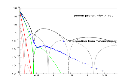
Two observations are in order concerning the $t$ behavior, the first is that at small $t$, the decrease is not an exponential and the cross-section is not decreasing fast enough, and the second is that the dip is not reproduced at all, neither in position nor in value. As mentioned, at very high energy, the shape of the curve reproduces a black disk model as one can see from the behavior of the amplitude in $b$-space, Fig.  4.

Figure 4: The BN amplitude in $b$-space, for different values of the singularity parameter $p$. The dashed red line indicates the values when $1-exp[-\bar{n}/2]=1/2$. Higher $p$ values correspond to innermost curves.

for a typical parametrization with GRV densities, $p_{tmin}=1.15\ GeV$ and different $p$ values at $\sqrt{s}=7\ TeV$. The red dashed line indicates the $b$-value at which the amplitude in $b$-space is such that ${\mathcal{A}}(b_{max},s)=1/2$. Then, one can approximate the amplitude with a black disk of radius $b_{max}$, so that

$$A^{BD}_{el}(s,t)\approx b_{max}^{2}\left[\frac{J_{1}(b_{max}\sqrt{-t})}{b_{max}\sqrt{-t}}\right]$$ (25)

and the dip occurs at the first zero of the $J_{1}$, located at $b_{max}\sqrt{-t_{dip}}\simeq 3.83$, leading to $-t_{dip}\simeq 14.7/b_{max}^{2}$. One sees that $b_{max}$ at a given energy depends on the value of the singularity parameter $p$: larger $p$ means more suppression, and smaller $b_{max}$. Thus we make a general point of physical relevance which follows directly from our ansatz of Eq. (11): ${\rm both}\ b_{max}\uparrow$ and $\sigma_{tot}\uparrow$ as $p\downarrow$.

The BN model corresponds to initial state emission of soft gluons from intermediate parton-parton scattering. A final rescattering has to be expected for the elastic cross-section at $t\neq 0$. In a model such as the one we are discussing, the only scale present is $b_{max}$ and to reproduce the forward peak, we apply to the amplitude a rescattering factor given by

$${\cal S}(s,t)=e^{tb^{2}_{max}(s,t)/4}\ \ \ \ \ \ \ {\cal S}(s,0)=1$$ (26)

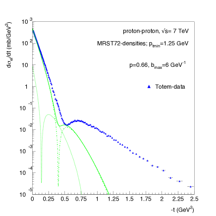
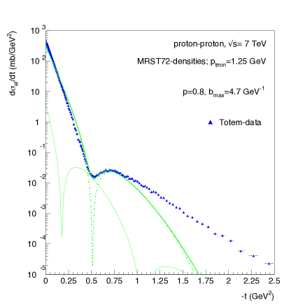
which corresponds to $b_{max}(s,t)$ being the value beyond which the amplitude in b-space falls below $1/2$. It is quite possible that $b_{max}$ depends on the momentum transfer $q^{2}$, with $b_{max}(s,t_{1})>b_{max}(s,t_{2})$ for $-t_{1}<-t_{2}$, but in the following we shall just consider it as a constant in $t$, namely we shall put $b_{max}\equiv b_{max}(s,0)$. The numerical value of $b_{max}$ is not well defined, since we could have chosen it to be the value where ${\mathcal{A}}(s,b)=[1-1/e]$ as, for instance in [14] and also because the BD approximation is not exact yet, at LHC7. Thus, the factor to be applied is here determined by trial and error. Multiplying the cross-section by the factor ${\cal S}(s,t)$ with $4.8<b_{max}<6\ GeV^{-1}$ gives the results shown in Fig.  5, obtained with mini-jets calculated with both MRST72 and GRV PDFs.

Figure 5: The result of applying the rescattering factor to the one-channel BN model, as described in the text. Bottom figures use GRV densities.

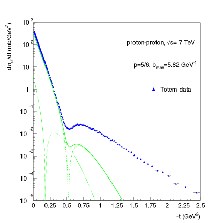
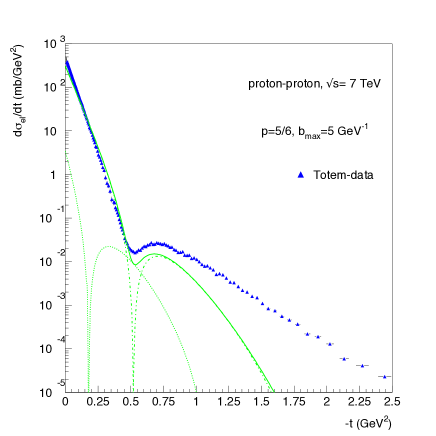
In particular:

• The two top figures are obtained with MRST72 densities, the top left corresponding to the parameter set which reproduces the total cross-section at LHC7, MRST72 PDF, $p=0.66,\ p_{tmin}=1.25\ GeV$ [6]. For the top left plot, we use the $p$ value which reproduces the optical point and the slope is obtained from the $b_{max}(p=0.66)$ value consistent with the behavior of $\bar{n}$ for the corresponding densities. However, the position of the dip is still too much to the left. To obtain a curve with the dip in the right position one needs an amplitude with a larger $p$ value, as in the right top plot, where the value for $b_{max}$ is chosen so as to reproduce the dip. The description of $\sigma_{elastic}$ with these densities is obtained with $p=0.8$, but then the optical point is lost.

• the bottom figures are an exercise in showing how the slope $b_{max}$ influences the depth of the dip: once a $p$-value is chosen so as obtain the correct dip position, by varying $b_{max}$ as a free parameter the curve can be lowered and the normalization at the dip can be correctly reproduced.

• The two bottom figures are obtained with a different PDF set, GRV, and parameter $p=5/6$, the value which would reproduce $\sigma_{elastic}$ with these densities: this allows to keep the position of the dip in the proper place. Lowering $b_{max}$ to a value $b_{max}=4.75\ GeV^{-1}$ will fully reproduce the dip with these densities.

In all these figures, except for the top left one, the optical point is not reproduced. The above confirms the well known fact that there is no geometrical scaling at these energies [15], namely the differential elastic cross-section does not scale with the variable $\tau=-t\ \sigma_{total}$. In particular the position of the dip is not given by $\tau_{dip}=-t_{dip}\ \sigma_{total}$. Until the BD limit of ${\cal R}_{el}=1/2$, the problem will have two scales, the total and the elastic cross-sections. In the empirical model of [16] it appears that this limit, if reached at all, may still be very far and in [2] we have proposed a different scaling behaviour for the position of the dip [17], namely

$$\tau_{dip}=-t\ \sqrt{\sigma_{tot}\sigma_{el}}=constant.$$ (27)

How to include this in a one channel eikonal model such as the above BN model, is under study. Notice that only recently we became aware of two previous works by Kawasaki, Maehara and Yonezawa [17] on the generalized form of geometrical scaling (GS) in elastic scattering at high energies.

Here we mention that a possible way to reconcile with the original GS is to account for the energy evolution of $\mathcal{R}_{el}(s)$, introducing a saturating function at $s\rightarrow\infty$ [18], as done in [19], for instance.

4 Conclusions

All of the above shows that in a one channel eikonal the position of the dip is inconsistent with the correct reproduction of the optical point. This is a well known fact, but we have discussed it in detail through our mini-jet with soft gluon resummation model, the BN model. It also corresponds to the fact that there is no geometrical scaling (at least for the energies probed as yet): $-t_{dip}\ \sigma_{total}$ is not a constant. We have discussed this point in a recent note [2] and refer the reader to the considerations exposed in that paper.

In addition to the above problems alluded to with this one-channel eikonal, the tail after the dip-bump region is also not reproduced at all. This clearly implies that a second term needs to be added, as shown through the results of our empirical model in [16], where we have described data for the elastic differential cross-section through two terms, one corresponding only to $C=+1$ exchange and a second one which includes $C=-1$ exchange, which is not present here. According to Donnachie and Landshoff, the behavior after the dip arises because of a perturbative contribution from three gluon exchanges, a $C=-1$ term [3]. Work is in progress to examine such a possibility in the context of this BN model.

References

- [1] G. Antchev et al., Measurement of proton-proton elastic scattering and total cross-section at = 7 TeV, , Europhys.Lett. 101 (2013) 21002.
- [2] G. Pancheri, D.A. Fagundes, A. Grau and Y.N. Srivastava, An empirical model for scattering and geometrical scaling, arXiv:1402.1844 [hep-ph].
- [3] A. Donnachie and P.V. Landshoff, and total cross sections and elastic scattering Phys.Lett. B727 (2013) 500-505, arXiv:1309.1292 [hep-ph].
- [4] A. Grau, G. Pancheri and Y.N. Srivastava, Hadronic total cross-sections through soft gluon summation in impact parameter space, Phys.Rev.D 60 (1999) 114020.
- [5] R.M. Godbole, A. Grau, G. Pancheri, Y.N. Srivastava, Soft gluon radiation and energy dependence of total hadronic cross-sections, Phys.Rev.D 72 (2005) 076001.
- [6] A. Achilli, R.M. Godbole, A. Grau, G. Pancheri and Y.N. Srivastava, Total and inelastic cross sections at LHC at TeV and beyond, Phys.Rev.D 84 (2011) 094009.
- [7] A. Achilli, R. Hegde, R. M. Godbole, A. Grau, G. Pancheri and Y. Srivastava, Total cross-section and rapidity gap survival probability at the LHC through an eikonal with soft gluon resummation, Phys.Lett.B 659 (2008) 137-143.
- [8] F. Bloch and A. Nordsieck, Note on the Radiation Field of the electron, Phys.Rev. 52 (1937) 54.
- [9] A. Corsetti, A. Grau, G. Pancheri and Y.N. Srivastava, Bloch-Nordsieck summation and partonic distributions in impact parameter space, Phys.Lett.B 382 (1996) 282-288.
- [10] A. Grau, R.M. Godbole, G. Pancheri and Y.N. Srivastava, Soft Gluon kt-Resummation and the Froissart bound, Phys.Lett.B 682 (2009) 55.
-
[11]
M. Gluck, E. Reya and A. Vogt, Parton distributions for high-energy collisions, Z.Phys.C 53 (1992) 651-656;
M. Gluck, E. Reya and A. Vogt, Dynamical parton distributions of the proton and small x physics, Z.Phys.C 67 (1995) 433-448;
M. Gluck, E. Reya and A. Vogt, Dynamical parton distributions revisited Eur.Phys.J.C 5 (1998) 461-470. - [12] A.D. Martin, R.G. Roberts, W.J. Stirling and R.S. Thorne, Scheme dependence, leading order and higher twist studies of MRST partons, Phys.Lett.B 443 (1998) 301-307.
- [13] A. Martin, Asymptotic behaviour of the real part of the scattering amplitude at , Lett.Nuovo Cim. 7S2 (1973) 811-812.
- [14] M.M. Block, Hadronic forward scattering: Predictions for the Large Hadron Collider and cosmic rays, Phys.Rept. 436 (2006) 71-215.
- [15] P. Brogueira, and J. Dias de Deus, Testing the Black Disk Limit in pp Collisions at Very High Energy , J.Phys.G 39 (2012) 055006.
- [16] D. A. Fagundes , A. Grau, S. Pacetti, G. Pancheri, and Y.N. Srivastava, Elastic pp scattering from the optical point to past the dip: an empirical parametrization from ISR to LHC, Phys.Rev. D88 (2013) 094019.
[17]
M. Kawasaki, T. Maehara and M. Yonezawa, Generalized geometrical scaling behavior of elastic hadron hadron scattering amplitudes at high-energies, Phys.Rev.D 48 (1993) 3098-3109;
M. Kawasaki, T. Maehara and M. Yonezawa, Generalized geometrical scaling for elastic hadron hadron scattering at high-energies, Phys.Rev.D 47 (1993) 3-6. - [18] D.A. Fagundes and M.J. Menon, Total Hadronic Cross Section and the Elastic Slope: An Almost Model-Independent Connection, Nucl.Phys.A 880 (2012) 1-11.
- [19] I. Bautista and J. Dias de Deus, The black disk and the dip in the differential elastic cross section at asymptotic energy , Phys.Lett.B 718 (2013) 1571.