On Hypothesis Testing for Poisson Processes. Singular Cases

Abstract

We consider the problem of hypothesis testing in the situation where the first hypothesis is simple and the second one is local one-sided composite. We describe the choice of the thresholds and the power functions of different tests when the intensity function of the observed inhomogeneous Poisson process has two different types of singularity: cusp and discontinuity. The asymptotic results are illustrated by numerical simulations.

MSC 2010 Classification: 62M02, 62F03, 62F05.

Key words: Hypothesis testing, inhomogeneous Poisson processes, asymptotic theory, composite alternatives, singular situations.

1 Introduction

This is the second part of the study devoted to hypothesis testing problems in the case when the observations are inhomogeneous Poisson processes. The first part was concerned with the regular (smooth) case [3], while this second part deals with non regular (singular) situations. We suppose that the intensity function of the observed inhomogeneous Poisson process depends on the unknown parameter $\vartheta$ in a non regular way (for example, the Fisher information is infinite). The basic hypothesis is always simple ($\vartheta=\vartheta_{1}$) and the alternative is one-sided composite ($\vartheta>\vartheta_{1}$). In the first part we studied the asymptotic behavior of the Score Function test (SFT), of the General Likelihood Ratio test (GLRT), of the Wald test (WT) and of two Bayes tests (BT1 and BT2). It was shown that the tests SFT, GLRT and WT are locally asymptotically uniformly most powerful. In the present work we study the asymptotic behavior of the GLRT, WT, BT1 and BT2 in two non regular situations. More precisely, we study the tests when the intensity functions has a cusp-type singularity or a jump-type singularity. In both cases the Fisher information is infinite. The local alternatives are obtained by the reparametrization $\vartheta=\vartheta_{1}+u\varphi_{n}$, $u>0$. The rate of convergence $\varphi_{n}\rightarrow 0$ depends on the type of singularity. In the cusp case $\varphi_{n}\sim n^{-\frac{1}{2\kappa+1}}$, where $\kappa$ is the order of the cusp, and in the discontinuous case $\varphi_{n}\sim n^{-1}$. Our goal is to describe the choice of the thresholds and the behavior of the power functions as $n\rightarrow\infty$. The important difference between regular and singular cases is the absence of the criteria of optimality. This leads to a situation when the comparison of the power functions can be only done numerically. That is why we present the results of numerical simulations of the limit power functions and the comparison of them with the power functions with small and large volumes of observations (small and large $n$).

Recall that $X=\left(X_{t},\ t\geq 0\right)$ is an inhomogeneous Poisson process with intensity function $\lambda\left(t\right)$, $t\geq 0$, if $X_{0}=0$ and the increments of $X$ on disjoint intervals are independent and distributed according to the Poisson law

$$\mathop{\mathbf{\kern 0.0ptP}}\nolimits\left\{X_{t}-X_{s}=k\right\}=\frac{\left(\int_{s}^{t}\lambda\left(t\right){\rm d}t\right)^{k}}{k!}\exp\left\{-\int_{s}^{t}\lambda\left(t\right){\rm d}t\right\}.$$

We suppose that the intensity function depends on some one-dimensional parameter, that is, $\lambda\left(t\right)=\lambda\left(\vartheta,t\right)$. The basic hypothesis is simple: $\vartheta=\vartheta_{1}$, while the alternative is one-sided composite: $\vartheta>\vartheta_{1}$.

The hypothesis testing problems for inhomogeneous Poisson processes were studied by many authors (see, for example, [12], [5], [3] and the references therein).

2 Preliminaries

We consider the model of $n$ independent observations of an inhomogeneous Poisson process: $X^{n}=\left(X_{1},\ldots,X_{n}\right)$, where $X_{j}=\left(X_{j}\left(t\right),0\leq t\leq\tau\right)$, $j=1,\ldots,n$, are Poisson processes with

$$\mathop{\mathbf{\kern 0.0ptE}}\nolimits_{\vartheta}X_{j}\left(t\right)=\Lambda\left(\vartheta,t\right)=\int_{0}^{t}\lambda\left(\vartheta,s\right)\;{\rm d}s.$$

We use here the same notations as in [3]. In particular, $\vartheta$ is one-dimensional parameter and $\mathop{\mathbf{\kern 0.0ptE}}\nolimits_{\vartheta}$ is the mathematical expectation in the case when the true value is $\vartheta$. The intensity function is supposed to be separated from zero on $\left[0,\tau\right]$. The measures corresponding to Poisson processes with different values of $\vartheta$ are equivalent and the likelihood function is defined by the equality

$$L(\vartheta,X^{n})=\exp\left\{\sum_{j=1}^{n}\int_{0}^{\tau}\ln\lambda\left(\vartheta,t\right){\rm d}X_{j}\left(t\right)-n\int_{0}^{\tau}\left[\lambda\left(\vartheta,t\right)-1\right]{\rm d}t\right\}.$$

In non-regular situations we do not have a LAUMP test, and it is interesting to compare the power functions of different tests with the power function of the Neyman-Pearson test (N-PT). Let us recall the definition of the N-PT. Suppose that we have two simple hypotheses $\mathscr{H}_{1}:\vartheta=\vartheta_{1}$ and $\mathscr{H}_{2}:\vartheta=\vartheta_{2}$ and our goal is to construct a test $\bar{\psi}_{n}\left(X^{n}\right)$ of size $\varepsilon$, that is, a test with given probability of the error of the first kind $\mathop{\mathbf{\kern 0.0ptE}}\nolimits_{\vartheta_{1}}\bar{\psi}_{n}\left(X^{n}\right)=\varepsilon$. As usually, the test $\bar{\psi}_{n}\left(X^{n}\right)$ is the probability to reject the hypothesis $\mathscr{H}_{1}$ and, of course, to accept the hypothesis $\mathscr{H}_{2}$.

Let us denote the likelihood ratio statistic as

$$L\left(\vartheta_{2},\vartheta_{1},X^{n}\right)=L\left(\vartheta_{2},X^{n}\right)/L\left(\vartheta_{1},X^{n}\right).$$

Then, by the Neyman-Pearson Lemma [13], the N-PT is

$$\psi_{n}^{*}\left(X^{n}\right)=\begin{cases}1,&\,{\rm if}\,\,\quad L\left(\vartheta_{2},\vartheta_{1},X^{n}\right)>d_{\varepsilon},\\ q_{\varepsilon},&\,{\rm if}\,\quad L\left(\vartheta_{2},\vartheta_{1},X^{n}\right)=d_{\varepsilon},\\ 0,&\,{\rm if}\,\quad L\left(\vartheta_{2},\vartheta_{1},X^{n}\right)<d_{\varepsilon},\end{cases}$$

where the constants $d_{\varepsilon}$ and $q_{\varepsilon}$ are solutions of the equation

$$\mathop{\mathbf{\kern 0.0ptP}}\nolimits_{\vartheta_{1}}\left(L\left(\vartheta_{2},\vartheta_{1},X^{n}\right)>d_{\varepsilon}\right)+q_{\varepsilon}\mathop{\mathbf{\kern 0.0ptP}}\nolimits_{\vartheta_{1}}\left(L\left(\vartheta_{2},\vartheta_{1},X^{n}\right)=d_{\varepsilon}\right)=\varepsilon.$$

In this work we consider the construction of the tests in the following hypothesis testing problem

$$\mathscr{H}_{1} :\qquad\vartheta=\vartheta_{1},$$ (1)

$$\mathscr{H}_{2} :\qquad\vartheta>\vartheta_{1},$$

that is, we have a simple hypothesis against one-sided composite alternative.

The log likelihood ratio function can be written as follows:

$$\ln L(\vartheta,\vartheta_{1},X^{n})=\sum_{j=1}^{n}\int_{0}^{\tau}\ln\frac{\lambda\left(\vartheta,t\right)}{\lambda\left(\vartheta_{1},t\right)}{\rm d}X_{j}\left(t\right)-n\int_{0}^{\tau}\left[\lambda\left(\vartheta,t\right)-\lambda\left(\vartheta_{1},t\right)\right]{\rm d}t.$$

The power function of a test $\bar{\psi}_{n}\left(X^{n}\right)$ is $\beta\left(\bar{\psi}_{n},\vartheta\right)=\mathop{\mathbf{\kern 0.0ptE}}\nolimits_{\vartheta}\bar{\psi}_{n}\left(X^{n}\right)$, $\vartheta>\vartheta_{1}$.

We denote $\mathcal{K}_{\varepsilon}$ the class of tests $\bar{\psi}_{n}$ of asymptotic size $\varepsilon$:

$$\mathcal{K}_{\varepsilon}=\left\{\bar{\psi}_{n}\quad:\quad\lim_{n\rightarrow\infty}\mathop{\mathbf{\kern 0.0ptE}}\nolimits_{\vartheta_{1}}\bar{\psi}_{n}\left(X^{n}\right)=\varepsilon\right\}.$$

In this work we study several tests which belong to the class $\mathcal{K}_{\varepsilon}$. To compare these tests by their power functions we consider, as usual, the approach of close or contiguous alternatives (since for any fixed alternative the power functions of all tests converge to the same value $1$). We put $\vartheta=\vartheta_{1}+\varphi_{n}u$, where $\varphi_{n}=\varphi_{n}\left(\vartheta_{1}\right)>0$. Here $\varphi_{n}\rightarrow 0$ and the rate of convergence depends on the type of singularity of the intensity function.

Now the initial problem of hypothesis testing can be rewritten as follows:

$$\mathscr{H}_{1} :\qquad u=0,$$ (2)

$$\mathscr{H}_{2} :\qquad u>0.$$

The considered tests are usually of the form

$$\bar{\psi}_{n}={\mathbb{1}}_{\left\{Y_{n}\left(X^{n}\right)>c_{\varepsilon}\right\}}+q_{\varepsilon}{\mathbb{1}}_{\left\{Y_{n}\left(X^{n}\right)=c_{\varepsilon}\right\}},$$

where the constant $c_{\varepsilon}$ is defined with the help of the limit random variable $Y$ (suppose that $Y_{n}\Longrightarrow Y$ under hypothesis $\mathscr{H}_{1}$) by

$$\mathop{\mathbf{\kern 0.0ptE}}\nolimits_{\vartheta_{1}}\bar{\psi}_{n}=\mathop{\mathbf{\kern 0.0ptP}}\nolimits_{\vartheta_{1}}\left\{Y_{n}\left(X^{n}\right)>c_{\varepsilon}\right\}+q_{\varepsilon}\mathop{\mathbf{\kern 0.0ptP}}\nolimits_{\vartheta_{1}}\left\{Y_{n}\left(X^{n}\right)=c_{\varepsilon}\right\}\longrightarrow\mathop{\mathbf{\kern 0.0ptP}}\nolimits_{\vartheta_{1}}\left\{Y>c_{\varepsilon}\right\}=\varepsilon$$

if the limit random variable $Y$ is continuous, and by

$$\mathop{\mathbf{\kern 0.0ptP}}\nolimits_{\vartheta_{1}}\left\{Y>c_{\varepsilon}\right\}+q_{\varepsilon}\mathop{\mathbf{\kern 0.0ptP}}\nolimits_{\vartheta_{1}}\left\{Y=c_{\varepsilon}\right\}=\varepsilon$$

if $Y$ has distribution function with jumps.

The corresponding power function will be denoted

$$\beta\left(\bar{\psi}_{n},u\right)=\mathop{\mathbf{\kern 0.0ptE}}\nolimits_{\vartheta_{1}+\varphi_{n}u}\,\bar{\psi}_{n},\qquad u>0,$$

and the comparison of the tests will be carried in terms of their limit power functions.

We consider two different non regular models. In both of them, the intensity function $\lambda\left(\vartheta,t\right)$ is not differentiable and the Fisher information is infinite. More precisely, we study the behavior of the tests in two situations. The first one is when the intensity function has a cusp-type singularity (it is continuous but not differentiable), and the second one is when it has a jump-type singularity (it is discontinuous). In both cases the intensity functions $\lambda\left(\vartheta,t\right)$ has no derivative at the point $t=\vartheta$.

Note that these statistical models were already studied before in the problems of parameter estimation (see [1] for the cusp-type singularity and [9] for discontinuous intensity function), so here we concentrate on the properties of the tests. The main tool is, of course, the limit behavior of the normalized likelihood ratio function, which was already established before in the mentioned works but in a slightly different settings. The proofs given in this work are mainly based on the results presented in [1] and [9].

Recall that in the non regular cases considered in this work we do not have a LAUMP tests, and that is why a special attention is paid to numerical simulations of the limit power functions.

3 Cusp-type singularity

Suppose that the intensity function of the observed Poison processes is

$$\lambda\left(\vartheta,t\right)=a\left|t-\vartheta\right|^{\kappa}+h\left(t\right),\qquad 0\leq t\leq\tau,\qquad\vartheta\in\Theta=[\vartheta_{1},b),$$

where $\kappa\in\left(0,1/2\right)$, $\vartheta_{1}>0$, $b\leq\tau$, $a\neq 0$, and $h\left(\cdot\right)$ is a known positive bounded function.

To study the local alternatives we introduce the normalizing function

$$\varphi_{n}=n^{-\frac{1}{2H}}\Gamma_{\vartheta_{1}}^{-\frac{1}{H}},\qquad\Gamma_{\vartheta_{1}}^{2}=\frac{2a^{2}B\left(\kappa+1,\kappa+1\right)}{h\left({\vartheta_{1}}\right)}\left[\frac{1}{\cos\left(\pi\kappa\right)}-1\right],$$

where $B\left(\cdot,\cdot\right)$ is the Beta-function and $H=\kappa+\frac{1}{2}$ is the Hurst parameter. As usually, the change of variables $\vartheta=\vartheta_{1}+\varphi_{n}{u}$ reduces the initial hypothesis testing problem (1) to the problem (2).

We introduce the stochastic process

$$Z\left(u\right)=\exp\left\{W^{H}\left(u\right)-\frac{\left|u\right|^{2H}}{2}\right\},\qquad u\in\mathbb{R},$$

where $W^{H}\left(\cdot\right)$ is a fractional Brownian motion. Further, we define the random variable $\hat{u}$ by the relation

$$Z\left(\hat{u}\right)=\sup_{v\geq 0}Z\left(u\right),$$

and we introduce $h_{\varepsilon}$ and $g_{\varepsilon}$ as the solutions of the equations

$$\mathop{\mathbf{\kern 0.0ptP}}\nolimits\left(Z\left(\hat{u}\right)>h_{\varepsilon}\right)=\varepsilon\quad\text{and}\quad\mathop{\mathbf{\kern 0.0ptP}}\nolimits\left(\hat{u}>g_{\varepsilon}\right)=\varepsilon$$ (3)

respectively.

Note that $(Z\left(u\right),\ u\geq 0)$ is the likelihood ratio of a similar hypothesis testing problem ($u=0$ against $u>0$) in the case of observations $\left(Y\left(t\right),\ t\geq 0\right)$ of the following type

$${\rm d}Y\left(t\right)={\mathbb{1}}_{\left\{t<u\right\}}\;{\rm d}t+{\rm d}W^{H}\left(t\right),\qquad t\geq 0.$$

The uniformly most powerful test in this problem does not exist, and we do not have a LAUMP tests in our problem.

3.1 GLRT

The GLRT is defined by the relations

$$\hat{\psi}_{n}\left(X^{n}\right)={\mathbb{1}}_{\left\{Q\left(X^{n}\right)>h_{\varepsilon}\right\}},$$

where $h_{\varepsilon}$ is the solution of the first of the equations (3),

$$Q\left(X^{n}\right)=\sup_{\vartheta>\vartheta_{1}}{L\left(\vartheta,\vartheta_{1},X^{n}\right)}=L\left(\hat{\vartheta}_{n},\vartheta_{1},X^{n}\right),$$

and $\hat{\vartheta}_{n}$ is the maximum likelihood estimator (MLE).

Let us introduce the function

$$\hat{\beta}\left(u_{*}\right)=\mathop{\mathbf{\kern 0.0ptP}}\nolimits\left\{\sup_{u>0}\left[W^{H}\left(u\right)-\frac{\left|u-u_{*}\right|^{2H}}{2}\right]>\ln h_{\varepsilon}-\frac{\left|u_{*}\right|^{2H}}{2}\right\},\quad u_{*}\geq 0.$$

The properties of the GLRT are given in the following Proposition.

Proposition 1.

The GLRT $\hat{\psi}_{n}\left(X^{n}\right)$ belongs to $\mathcal{K}_{\varepsilon}$ and its power function in the case of local alternatives $\vartheta=\vartheta_{1}+\varphi_{n}u_{*}$, $u_{*}>0$, has the following limit:

$$\beta\left(\hat{\psi}_{n},u_{*}\right)\longrightarrow\hat{\beta}\left(u_{*}\right).$$

Proof.

Introduce the normalized likelihood ratio process

$$Z_{n}\left(u\right)=L\left(\vartheta_{1}+\varphi_{n}u,X^{n}\right)=\frac{L\left(\vartheta_{1}+\varphi_{n}u,X^{n}\right)}{L\left(\vartheta_{1},X^{n}\right)},\ \>\ u\in\mathbb{U}_{n}^{+}=\bigl{[}0,\varphi_{n}^{-1}\left(b-\vartheta_{1}\right)\bigr{)},$$

and let the function $Z_{n}\left(u\right)$ be linearly decreasing to zero on the interval $\left[\varphi_{n}^{-1}\left(b-\vartheta_{1}\right),\varphi_{n}^{-1}\left(b-\vartheta_{1}\right)+1\right]$ and equal to $0$ for all $u>\varphi_{n}^{-1}\left(b-\vartheta_{1}\right)+1$. Now the random function $Z_{n}\left(\cdot\right)$ is defined on $\mathbb{R}_{+}$.

Let us fix some $d\leq 0$ and denote $\mathscr{C}_{d}=\mathscr{C}_{d}\left(\mathbb{R}_{d}\right)$ the space of continuous functions on $\mathbb{R}_{d}=[d,\infty)$ with the property $\lim_{v\rightarrow\infty}z\left(v\right)=0$. Introduce the uniform metric on this space and denote $\mathcal{B}$ the corresponding Borel $\sigma$-algebra.

When we study the likelihood ratio process under hypothesis $\mathscr{H}_{1}$, we take $d=0$ and consider the corresponding measurable space $\left(\mathscr{C}_{0},\mathcal{B}\right)$. Under the alternative $\vartheta=\vartheta_{u_{*}}=\vartheta_{1}+\varphi_{n}u_{*}$, $u_{*}>0$, we will use this space with $d=-u_{*}$.

Let ${\bf Q}$ be the measure induced on the measurable space $\left(\mathscr{C}_{0},\mathcal{B}\right)$ by the stochastic processes $(Z\left(u\right),\ u\geq 0)$, and ${\bf Q}_{n}^{(\vartheta)}$ be the measure induced (under the true value $\vartheta$) on the same space by the processes $(Z_{n}\left(u\right),\ u\geq 0)$. The continuity with probability $1$ of the random functions $(Z_{n}\left(u\right),\ u\geq 0)$ follows from the inequality (6) below and the Kolmogorov theorem.

Suppose that we already proved the following weak convergence

$${\bf Q}_{n}^{(\vartheta_{1})}\Longrightarrow{\bf Q}.$$ (4)

Then the distribution of any continuous in the uniform metric functional $\Phi\left(Z_{n}\right)$ converge to the distribution of $\Phi\left(Z\right)$. In particular, if we take

$$\Phi\left(z\right)=\sup_{u\geq 0}z\left(u\right)-h_{\varepsilon},$$

we obtain

$$\mathop{\mathbf{\kern 0.0ptP}}\nolimits_{\vartheta_{1}}\left\{\sup_{\vartheta>\vartheta_{1}}{L\left(\vartheta,\vartheta_{1},X^{n}\right)}>h_{\varepsilon}\right\} =\mathop{\mathbf{\kern 0.0ptP}}\nolimits_{\vartheta_{1}}\left\{\sup_{u>0}Z_{n}\left(u\right)>h_{\varepsilon}\right\}$$

$$\longrightarrow{} \mathop{\mathbf{\kern 0.0ptP}}\nolimits\left\{\sup_{u>0}Z\left(u\right)>h_{\varepsilon}\right\}=\mathop{\mathbf{\kern 0.0ptP}}\nolimits\left\{Z\left(\hat{u}\right)>h_{\varepsilon}\right\}=\varepsilon.$$

Therefore the test $\hat{\psi}_{n}\in\mathcal{K}_{\varepsilon}$.

Let us note, that we do not know an analytic solution of the equation defining the constant $h_{\varepsilon}$, that is why below we turn to numerical simulations (see Section 3.4). Note also that $h_{\varepsilon}=h_{\varepsilon}\left(H\right)$ and does not depend on $\Gamma_{\vartheta_{1}}$.

To study the power function we consider the same likelihood ratio process but under the alternative $\vartheta_{u_{*}}=\vartheta_{1}+\varphi_{n}u_{*}$. We can write

$$Z_{n}\left(u\right) =\frac{L\left(\vartheta_{1}+\varphi_{n}u,X^{n}\right)}{L\left(\vartheta_{1},X^{n}\right)}=\frac{L\left(\vartheta_{u_{*}},X^{n}\right)}{L\left(\vartheta_{1},X^{n}\right)}\frac{L\left(\vartheta_{1}+\varphi_{n}u,X^{n}\right)}{L\left(\vartheta_{u_{*}},X^{n}\right)}$$

$$=\left(\frac{L\left(\vartheta_{u_{*}}-\varphi_{n}u_{*},X^{n}\right)}{L\left(\vartheta_{u_{*}},X^{n}\right)}\right)^{-1}\frac{L\left(\vartheta_{u_{*}}+(u-u_{*})\varphi_{n},X^{n}\right)}{L\left(\vartheta_{u_{*}},X^{n}\right)}$$

$$=\tilde{Z}_{n}\left(-u_{*}\right)^{-1}\tilde{Z}_{n}\left(u-u_{*}\right)$$

with an obvious notation. The difference between $Z_{n}\left(\cdot\right)$ and $\tilde{Z}_{n}\left(\cdot\right)$ is that the “reference value” in the first case is fixed (is equal to $\vartheta_{1}$) and in the second case it is “moving” (is equal to $\vartheta_{u_{*}}=\vartheta_{1}+\varphi_{n}u_{*}$). The random variable $\tilde{Z}_{n}\left(-u_{*}\right)$ converge in distribution to $Z\left(-u_{*}\right)$. For the stochastic process $(\tilde{Z}_{n}\left(u-u_{*}\right),\ u\geq 0)$ we have a similar convergence, and so, for any fixed $u\geq 0$, we have

$$\left(\tilde{Z}_{n}\left(-u_{*}\right),\tilde{Z}_{n}\left(u-u_{*}\right)\right)\Longrightarrow\left(Z\left(-u_{*}\right),Z\left(u-u_{*}\right)\right).$$

Now, let $\tilde{\bf Q}$ be the measure induced on the measurable space $\left(\mathscr{C}_{-u_{*}},\mathcal{B}\right)$ by the stochastic processes $(Z\left(u\right),\ u\geq-u_{*})$, and $\tilde{\bf Q}_{n}^{(\vartheta)}$ be the measure induced (under the true value $\vartheta$) on the same space by the stochastic processes $(\tilde{Z}_{n}\left(u\right),\ u\geq-u_{*})$. Suppose that we already proved the weak convergence

$$\tilde{\bf Q}_{n}^{(\vartheta_{u_{*}})}\Longrightarrow\tilde{\bf Q}.$$ (5)

Then for the power function we can write

$$\mathop{\mathbf{\kern 0.0ptP}}\nolimits_{\vartheta_{u_{*}}}\left\{\sup_{u>0}Z_{n}\left(u\right)>h_{\varepsilon}\right\}$$

$$\quad=\mathop{\mathbf{\kern 0.0ptP}}\nolimits_{\vartheta_{u_{*}}}\left\{\tilde{Z}_{n}\left(-u_{*}\right)^{-1}\sup_{u>0}\frac{L\left(\vartheta_{u_{*}}+(u-u_{*})\varphi_{n},X^{n}\right)}{L\left(\vartheta_{u_{*}},X^{n}\right)}>h_{\varepsilon}\right\}$$

$$\quad\longrightarrow\mathop{\mathbf{\kern 0.0ptP}}\nolimits\left\{Z\left(-u_{*}\right)^{-1}\sup_{u>0}\ \exp\left\{W^{H}\left(u-u_{*}\right)-\frac{\left|u-u_{*}\right|^{2H}}{2}\right\}>h_{\varepsilon}\right\}$$

$$\quad=\mathop{\mathbf{\kern 0.0ptP}}\nolimits\left\{\sup_{u>0}\left[-W^{H}\left(-u_{*}\right)+W^{H}\left(u-u_{*}\right)-\frac{\left|u-u_{*}\right|^{2H}}{2}+\frac{\left|u_{*}\right|^{2H}}{2}\right]>\ln h_{\varepsilon}\!\right\}$$

$$\quad=\mathop{\mathbf{\kern 0.0ptP}}\nolimits\left\{\sup_{u>0}\left[W^{H}\left(u\right)-\frac{\left|u-u_{*}\right|^{2H}}{2}\right]>\ln h_{\varepsilon}-\frac{\left|u_{*}\right|^{2H}}{2}\right\}=\hat{\beta}\left(u_{*}\right).$$

This limit power function is obtained below with the help of numerical simulations (see Section 3.4).

Let us also note that the limit (under the alternative $\vartheta_{u_{*}}=\vartheta_{1}+\varphi_{n}u_{*}$) of the likelihood ratio process $\left(Z_{n}\left(u\right),\ u\geq 0\right)$ is the process $\left(Z\left(u,u_{*}\right),\ u\geq 0\right)$ defined by

$$Z(u,u_{*})=W^{H}\left(u\right)-\frac{\left|u-u_{*}\right|^{2H}}{2}+\frac{\left|u_{*}\right|^{2H}}{2}.$$

To finish the proof we need to verify the convergence (5). To do this we follow the proof of the convergence (4) given in [1]. We introduce the following relations.

1. The finite-dimensional distributions of $(\tilde{Z}_{n}\left(u\right),\ u\geq-u_{*})$ converge to those of $\left(Z\left(u\right),\ u\geq-u_{*}\right)$.

2. There exists a positive constant $C$ such that

   $$\mathop{\mathbf{\kern 0.0ptE}}\nolimits_{\vartheta_{u_{*}}}\left|\tilde{Z}_{n}^{1/2}\left(u_{2}\right)-\tilde{Z}_{n}^{1/2}\left(u_{1}\right)\right|^{2}\leq C\,\left|u_{2}-u_{1}\right|^{2H},\qquad u_{1},u_{2}\geq-u_{*}.$$ (6)

3. There exists a positive constant $c$ such that

   $$\mathop{\mathbf{\kern 0.0ptE}}\nolimits_{\vartheta_{u_{*}}}\tilde{Z}_{n}^{1/2}\left(u\right)\leq\exp\left\{-c\left|u-u_{*}\right|^{2H}\right\},\qquad u\geq-u_{*}.$$ (7)

The proofs of these relations are slight modifications of the proofs given in [1]. Note that the characteristic function of the vector

$$\tilde{Z}_{n}\left(u_{1}\right),\ldots,\tilde{Z}_{n}\left(u_{k}\right)$$

can be written explicitly and the convergence of this characteristic function to the corresponding limit characteristic function can be checked directly (see Lemma 5 of [1]). The inequalities (6) and (7) follow from the Lemma 6 and Lemma 7 of [1] respectively.

These relations allow us to obtain the weak convergence (5) by applying the Theorem 1.10.1 of [7]. Note that the convergence (4) is a particular case of (5) with $u_{*}=0$. ∎

3.2 Wald test

Recall that the MLE $\hat{\vartheta}_{n}$ is defined by the equation

$$L\left(\hat{\vartheta}_{n},\vartheta_{1},X^{n}\right)=\sup_{\vartheta\in\Theta}L\left(\vartheta,\vartheta_{1},X^{n}\right).$$

The Wald test (WT) has the following form:

$$\psi_{n}^{\circ}\left(X^{n}\right)={\mathbb{1}}_{\left\{\varphi_{n}^{-1}\left(\hat{\vartheta}_{n}-\vartheta_{1}\right)>g_{\varepsilon}\right\}},$$

where $g_{\varepsilon}$ is the solution of the second of the equations (3).

Introduce as well the random variable $\hat{u}_{*}$ as solution of the equation

$$Z\left(\hat{u}_{*}\right)=\sup_{u\geq-u_{*}}Z\left(u\right).$$

Proposition 2.

The WT $\psi_{n}^{\circ}\left(X^{n}\right)$ belongs to $\mathcal{K}_{\varepsilon}$ and its power function in the case of local alternatives $\vartheta=\vartheta_{1}+\varphi_{n}u_{*}$, $u_{*}>0$, has the following limit:

$$\beta\left(\psi_{n}^{\circ},u_{*}\right)\longrightarrow\beta^{\circ}\left(u_{*}\right)=\mathop{\mathbf{\kern 0.0ptP}}\nolimits\left(\hat{u}_{*}>g_{\varepsilon}-u_{*}\right).$$

Proof.

The MLE (under hypothesis $\mathscr{H}_{1}$) converges in distribution

$$\varphi_{n}^{-1}\left(\hat{\vartheta}_{n}-\vartheta_{1}\right)\Longrightarrow\hat{u}.$$

Hence $\psi_{n}^{\circ}\in\mathcal{K}_{\varepsilon}$. For the proof see [1]. Recall that this convergence is a consequence of the weak convergence (4).

Let us study this estimator under the alternative $\vartheta_{u_{*}}=\vartheta_{1}+\varphi_{n}u_{*}$, $u_{*}>0$. We have

$$\mathop{\mathbf{\kern 0.0ptP}}\nolimits_{\vartheta_{u_{*}}}\left(\varphi_{n}^{-1}\left(\hat{\vartheta}_{n}-\vartheta_{u_{*}}\right)<x\right)$$

$$\>\ =\mathop{\mathbf{\kern 0.0ptP}}\nolimits_{\vartheta_{u_{*}}}\left(\sup_{\varphi_{n}^{-1}\left(\theta-\vartheta_{u_{*}}\right)<x}L\left(\theta,\vartheta_{u_{*}},X^{n}\right)>\sup_{\varphi_{n}^{-1}\left(\theta-\vartheta_{u_{*}}\right)\geq x}L\left(\theta,\vartheta_{u_{*}},X^{n}\right)\right)$$

$$\>\ =\mathop{\mathbf{\kern 0.0ptP}}\nolimits_{\vartheta_{u_{*}}}\left(\sup_{-u_{*}\leq u<x}\tilde{Z}_{n}\left(u\right)>\sup_{u\geq x}\tilde{Z}_{n}\left(u\right)\right)\longrightarrow\mathop{\mathbf{\kern 0.0ptP}}\nolimits\left(\sup_{-u_{*}\leq u<x}Z\left(u\right)>\sup_{u\geq x}Z\left(u\right)\right)$$

$$\>\ =\mathop{\mathbf{\kern 0.0ptP}}\nolimits\left(\hat{u}_{*}<x\right).$$

Here, as before,

$$\tilde{Z}_{n}\left(u\right)=\frac{L\left(\vartheta_{u_{*}}+\varphi_{n}u,X^{n}\right)}{L\left(\vartheta_{u_{*}},X^{n}\right)},\qquad u\geq-u_{*}.$$

Now, the limit of the power function of the WT is deduced from this convergence:

$$\beta\left(\psi_{n}^{\circ},u_{*}\right) =\mathop{\mathbf{\kern 0.0ptP}}\nolimits_{\vartheta_{u_{*}}}\left\{\varphi_{n}^{-1}\left(\hat{\vartheta}_{n}-\vartheta_{u_{*}}\right)+u_{*}>g_{\varepsilon}\right\}$$

$$\longrightarrow\mathop{\mathbf{\kern 0.0ptP}}\nolimits\left\{\hat{u}_{*}>g_{\varepsilon}-u_{*}\right\}=\beta^{\circ}\left(u_{*}\right),$$

which concludes the proof. ∎

Let us note, that we can also give another representation of the limit power function using the process $\left(Z\left(u,u_{*}\right),\ u\geq 0\right)$:

$$\beta\left(\psi_{n}^{\circ},u_{*}\right)\longrightarrow\mathop{\mathbf{\kern 0.0ptP}}\nolimits\left\{\hat{u}^{*}>g_{\varepsilon}\right\}=\beta^{\circ}\left(u_{*}\right),$$

where $\hat{u}^{*}$ is solution of the equation

$$Z\left(\hat{u}^{*}\right)=\sup_{u\geq 0}Z\left(u,u_{*}\right).$$

The threshold $g_{\varepsilon}$ and the power function $\beta^{\circ}\left(\cdot\right)$ are obtained below by numerical simulations (see Section 3.4).

3.3 Bayes tests

Suppose that the parameter $\vartheta$ is a random variable with a priori density $p\left(\theta\right)$, $\vartheta_{1}\leq\theta<b$. This function is supposed to be continuous and positive.

We consider two Bayes tests. The first one is based on the Bayes estimator, while the second one is based on the averaged likelihood ratio.

The first test, which we call BT1, is similar to WT, but is based on the Bayes estimator (BE) rather than on the MLE. Suppose that the loss function is quadratic. Then the BE $\tilde{\vartheta}_{n}$ is given by the following conditional expectation:

$$\tilde{\vartheta}_{n}=\int_{\vartheta_{1}}^{b}\theta p\left(\theta|X^{n}\right){\rm d}\theta=\frac{\int_{\vartheta_{1}}^{b}\theta p\left(\theta\right)L\left(\theta,X^{n}\right){\rm d}\theta}{\int_{\vartheta_{1}}^{b}p\left(\theta\right)L\left(\theta,X^{n}\right){\rm d}\theta}.$$

We introduce the test BT1 as

$$\tilde{\psi}_{n}\left(X^{n}\right)={\mathbb{1}}_{\left\{\varphi_{n}^{-1}\left(\tilde{\vartheta}_{n}-\vartheta_{1}\right)>k_{\varepsilon}\right\}},$$

where the constant $k_{\varepsilon}$ is solution of the equation

$$\mathop{\mathbf{\kern 0.0ptP}}\nolimits\left(\tilde{u}>k_{\varepsilon}\right)=\varepsilon,\qquad\tilde{u}=\frac{\int_{0}^{\infty}vZ\left(v\right){\rm d}v}{\int_{0}^{\infty}Z\left(v\right){\rm d}v}.$$

Introduce as well the function

$$\tilde{\beta}\left(u_{*}\right)=\mathop{\mathbf{\kern 0.0ptP}}\nolimits\left(\tilde{u}_{*}>k_{\varepsilon}-u_{*}\right),\qquad\tilde{u}_{*}=\frac{\int_{-u_{*}}^{\infty}vZ\left(v\right){\rm d}v}{\int_{-u_{*}}^{\infty}Z\left(v\right){\rm d}v},\qquad u_{*}\geq 0.$$

Proposition 3.

The BT1 $\tilde{\psi}_{n}\left(X^{n}\right)$ belongs to $\mathcal{K}_{\varepsilon}$ and its power function in the case of local alternatives $\vartheta=\vartheta_{1}+\varphi_{n}u_{*}$, $u_{*}>0$, has the following limit:

$$\beta\left(\tilde{\psi}_{n},u_{*}\right)\longrightarrow\tilde{\beta}\left(u_{*}\right).$$

Proof.

The Bayes estimator $\tilde{\vartheta}_{n}$ is consistent and has the following limit distribution (under hypothesis $\mathscr{H}_{1}$)

$$\varphi_{n}^{-1}\left(\tilde{\vartheta}_{n}-\vartheta_{1}\right)\Longrightarrow\tilde{u}$$

(for the proof see [1]). Hence $\tilde{\psi}_{n}\left(X^{n}\right)\in\mathcal{K}_{\varepsilon}$.

For the power function we have

$$\beta\left(\tilde{\psi}_{n},u_{*}\right) =\mathop{\mathbf{\kern 0.0ptP}}\nolimits_{\vartheta_{u_{*}}}\left\{\varphi_{n}^{-1}\left(\tilde{\vartheta}_{n}-\vartheta_{1}\right)>k_{\varepsilon}\right\}$$

$$=\mathop{\mathbf{\kern 0.0ptP}}\nolimits_{\vartheta_{u_{*}}}\left\{\varphi_{n}^{-1}\left(\tilde{\vartheta}_{n}-\vartheta_{u_{*}}\right)>k_{\varepsilon}-u_{*}\right\}.$$

Let us study the normalized difference $\tilde{u}_{n}=\varphi_{n}^{-1}\left(\tilde{\vartheta}_{n}-\vartheta_{u_{*}}\right)$. We can write (using the change of variables $\theta=\vartheta_{u_{*}}+\varphi_{n}v$)

$$\int_{\vartheta_{1}}^{b}\theta p\left(\theta\right)L\left(\theta,\vartheta_{u_{*}},X^{n}\right){\rm d}\theta$$

$$\qquad=\varphi_{n}\int_{-u_{*}}^{\varphi_{n}^{-1}\left(b-\vartheta_{u_{*}}\right)}\left(\vartheta_{u_{*}}+\varphi_{n}v\right)p\left(\vartheta_{u_{*}}+\varphi_{n}v\right)L\left(\vartheta_{u_{*}}+\varphi_{n}v,\vartheta_{u_{*}},X^{n}\right){\rm d}v$$

$$\qquad=\varphi_{n}\int_{-u_{*}}^{\varphi_{n}^{-1}\left(b-\vartheta_{u_{*}}\right)}\left(\vartheta_{u_{*}}+\varphi_{n}v\right)p\left(\vartheta_{u_{*}}+\varphi_{n}v\right)\tilde{Z}_{n}\left(v\right){\rm d}v.$$

Hence

$$\tilde{u}_{n}=\frac{\int_{-u_{*}}^{\varphi_{n}^{-1}\left(b-\vartheta_{u_{*}}\right)}vp\left(\vartheta_{u_{*}}+\varphi_{n}v\right)\tilde{Z}_{n}\left(v\right){\rm d}v}{\int_{-u_{*}}^{\varphi_{n}^{-1}\left(b-\vartheta_{u_{*}}\right)}p\left(\vartheta_{u_{*}}+\varphi_{n}v\right)\tilde{Z}_{n}\left(v\right){\rm d}v}\Longrightarrow\frac{\int_{-u_{*}}^{\infty}vZ\left(v\right){\rm d}v}{\int_{-u_{*}}^{\infty}Z\left(v\right){\rm d}v}=\tilde{u}_{*}$$

(since $p\left(\vartheta_{u_{*}}+\varphi_{n}v\right)\longrightarrow p\left(\vartheta_{1}\right)>0$ and $\tilde{Z}_{n}\Longrightarrow Z$). The detailed proof is based on the properties 1–3 of the likelihood ratio (see [1] or [7, Theorem 1.10.2]). ∎

Let us note, that we can also give another representation of the limit power function using the process $\left(Z\left(u,u_{*}\right),\ u\geq 0\right)$:

$$\beta\left(\tilde{\psi}_{n},u_{*}\right)\longrightarrow\mathop{\mathbf{\kern 0.0ptP}}\nolimits\left(\tilde{u}^{*}>k_{\varepsilon}\right)=\tilde{\beta}\left(u_{*}\right),$$

where $\displaystyle\tilde{u}^{*}=\frac{\int_{0}^{\infty}vZ\left(v,u_{*}\right){\rm d}v}{\int_{0}^{\infty}Z\left(v,u_{*}\right){\rm d}v}$.

The second test, which we call BT2, is given by

$$\tilde{\psi}_{n}^{\star}\left(X^{n}\right)={\mathbb{1}}_{\left\{R_{n}\left(X^{n}\right)>m_{\varepsilon}\right\}},\qquad R_{n}\left(X^{n}\right)=\frac{\tilde{L}_{n}\left(X^{n}\right)}{p\left(\vartheta_{1}\right)\varphi_{n}}.$$

Here

$$\tilde{L}_{n}\left(X^{n}\right)=\int_{\vartheta_{1}}^{b}L\left(\theta,\vartheta_{1},X^{n}\right)p\left(\theta\right){\rm d}\theta,$$

and $m_{\varepsilon}$ is solution of the equation

$$\mathop{\mathbf{\kern 0.0ptP}}\nolimits\left\{\int_{0}^{\infty}Z\left(v\right){\rm d}v>m_{\varepsilon}\right\}=\varepsilon.$$

Introduce as well the function

$$\tilde{\beta}^{\star}\left(u_{*}\right)=\mathop{\mathbf{\kern 0.0ptP}}\nolimits\left(Z\left(-u_{*}\right)^{-1}\int_{-u_{*}}^{\infty}Z\left(v\right)\,{\rm d}v>m_{\varepsilon}\right).$$

Proposition 4.

The BT2 $\tilde{\psi}_{n}^{\star}\left(X^{n}\right)$ belongs to $\mathcal{K}_{\varepsilon}$ and its power function in the case of local alternatives $\vartheta=\vartheta_{1}+\varphi_{n}u_{*}$, $u_{*}>0$, has the following limit:

$$\beta\left(\tilde{\psi}_{n}^{\star},u_{*}\right)\longrightarrow\tilde{\beta}^{\star}\left(u_{*}\right).$$

Proof.

Let us first recall how this test was obtained. Introduce the mean error of the second kind $\bar{\alpha}\left(\bar{\psi}_{n}\right)$ under alternative $\mathscr{H}_{2}$ of an arbitrary test $\bar{\psi}_{n}$ as

$$\bar{\alpha}\left(\bar{\psi}_{n}\right)=\int_{\vartheta_{1}}^{b}\mathop{\mathbf{\kern 0.0ptE}}\nolimits_{\theta}\bar{\psi}_{n}\left(X^{n}\right)\,p\left(\theta\right)\,{\rm d}\theta=\mathop{\mathbb{\kern 0.0ptE}}\nolimits\bar{\psi}_{n},$$

where $\mathop{\mathbb{\kern 0.0ptE}}\nolimits$ is the double mathematical expectation, that is, the expectation with respect to the measure

$$\mathop{\mathbb{\kern 0.0ptP}}\nolimits\left(X^{n}\in A\right)=\int_{\vartheta_{1}}^{b}\mathop{\mathbf{\kern 0.0ptP}}\nolimits_{\theta}\left(X^{n}\in A\right)p\left(\theta\right)\,{\rm d}\theta.$$

If we consider the problem of the minimization of this mean error, we reduce the initial hypothesis testing problem to the problem of testing of two simple hypotheses

$$\mathscr{H}_{1}\quad:\quad X^{n}\quad\sim\quad\mathop{\mathbf{\kern 0.0ptP}}\nolimits_{\vartheta_{1}},$$

$$\mathscr{H}_{2}\quad:\quad X^{n}\quad\sim\quad\mathop{\mathbb{\kern 0.0ptP}}\nolimits.$$

Then, by the Neyman-Pearson Lemma, the most powerful test in the class $\mathcal{K}_{\varepsilon}$ $\bigl{(}$which minimizes the mean error $\bar{\alpha}\bigl{(}\bar{\psi}_{n}\bigr{)}\bigr{)}$ is

$$\tilde{\psi}_{n}^{*}\left(X^{n}\right)={\mathbb{1}}_{\left\{\tilde{L}_{n}\left(X^{n}\right)>\tilde{m}_{\varepsilon}\right\}},$$

where the averaged likelihood ratio

$$\tilde{L}_{n}\left(X^{n}\right)=\frac{{\rm d}\mathop{\mathbb{\kern 0.0ptP}}\nolimits\hfill}{{\rm d}\mathop{\mathbf{\kern 0.0ptP}}\nolimits_{\vartheta_{1}}}\left(X^{n}\right)=\varphi_{n}\int_{0}^{\varphi_{n}^{-1}\left(\beta-\vartheta_{1}\right)}Z_{n}\left(v\right)p\left(\vartheta_{1}+v\varphi_{n}\right){\rm d}v$$

and $\tilde{m}_{\varepsilon}$ is chosen from the condition $\tilde{\psi}_{n}^{*}\in\mathcal{K}_{\varepsilon}$. Now, it is clear that the BT2 $\tilde{\psi}_{n}^{\star}\left(X^{n}\right)$ coincides with the test $\tilde{\psi}_{n}^{*}\left(X^{n}\right)$ if we put $\tilde{m}_{\varepsilon}=m_{\varepsilon}\,p\left(\vartheta_{1}\right)\varphi_{n}$.

In the proof of the convergence in distribution of the Bayes estimator it is shown (see [7, Theorem 1.10.2] and [1]) that

$$\varphi_{n}^{-1}\tilde{L}\left(X^{n}\right)\Longrightarrow p\left(\vartheta_{1}\right)\int_{0}^{\infty}Z\left(v\right){\rm d}v.$$

Therefore (under hypothesis $\mathscr{H}_{1}$),

$$R_{n}\left(X^{n}\right)\Longrightarrow\int_{0}^{\infty}Z\left(v\right)\,{\rm d}v$$

and the test $\tilde{\psi}_{n}^{\star}\left(X^{n}\right)$ belongs to the class $\mathcal{K}_{\varepsilon}$.

Using a similar argument, we can verify the convergence

$$R_{n}\left(X^{n}\right)\Longrightarrow Z\left(-u_{*}\right)^{-1}\int_{-u_{*}}^{\infty}Z\left(v\right)\,{\rm d}v$$

under the alternative $\vartheta_{u_{*}}$, which concludes the proof. ∎

3.4 Simulations

Let us consider the following example. We observe $n$ independent realizations $X^{n}=\left(X_{1},\ldots,X_{n}\right)$, where $X_{j}=\left(X_{j}(t),\ t\in\left[0,2\right]\right)$, $j=1,\ldots,n$, of an inhomogeneous Poisson process. The intensity function of this processes is

$$\lambda(\vartheta,t)=2-\left|t-\vartheta\right|^{0.4},\qquad 0\leq t\leq 2,$$

where the parameter $\vartheta\in\left[0.5,2\right)$. We take $\vartheta_{1}=1.5$ as the value of the basic hypothesis $\mathscr{H}_{1}$. Of course it is sufficient to have simulations for the values $\vartheta\in\left[1.5,2\right)$, but we consider a wider interval to show the behavior of the likelihood ratio on the both sides of the true value. The Hurst parameter is $H=0.9$ and the constant $\Gamma^{2}_{\vartheta_{1}}=B(1.4,1.4)\Bigl{[}\frac{1}{\cos(0.4\pi)}-1\Bigr{]}\approx 1.027$.

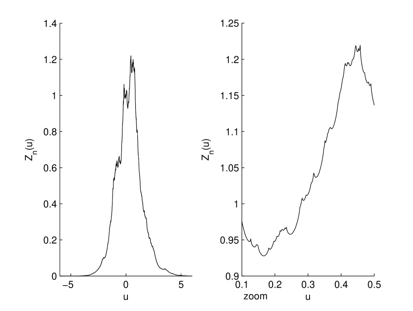
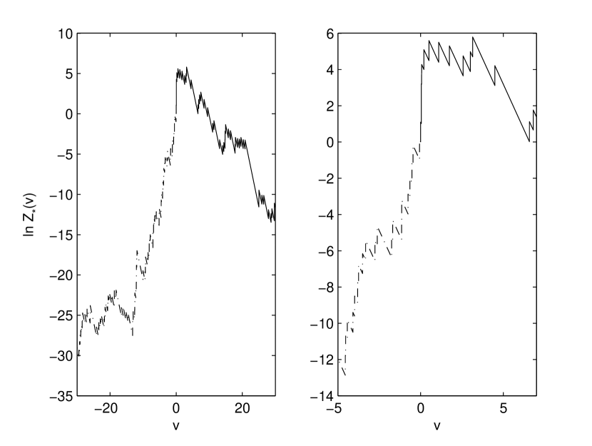
A realization of the normalized likelihood ratio $Z_{n}\left(u\right)$, $u\in\left[-5,5\right]$, and its zoom $Z_{n}\left(u\right)$, $u\in\left[0.1,0.5\right]$, under the hypothesis $\mathscr{H}_{1}$ are given in Figure 1.

 Here Figure 1  

To find the thresholds of the GLRT and of the WT, we need to find the point of maximum and the maximal value of this function. In the case of the chosen intensity function, the maximum is attained at one of the cusps of the likelihood ratio (that is, on one of the events of one of the observed Poisson processes).

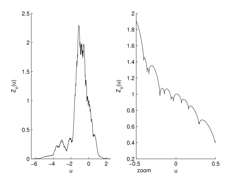
It is interesting to note that if the intensity function has the same singularity but with a different sign: $\lambda\left(\vartheta,t\right)=0.5+\left|t-\vartheta\right|^{0.4}$, then it is much more difficult to find the maximum (see Figure 2).

 Here Figure 2.  

The thresholds of the GLRT, of the WT and of the BT1 are presented in Table 1.

$\varepsilon$	0.01	0.05	0.10	0.2	0.4	0.5
$\ln h_{\varepsilon}$	2.959	1.641	1.081	0.559	0.159	0.068
$g_{\varepsilon}$	3.041	1.996	1.521	0.950	0.333	0.166
$k_{\varepsilon}$	2.864	2.0776	1.720	1.365	1.005	0.885

Table 1: Thresholds of GLRT, WT and BT1

For example, the thresholds of the GLRT are obtained by simulating $M=10^{5}$ trajectories of $Z^{i}(u)$, $u\in\left[0,20\right]$, $i=1,\ldots,M$ (when $u>20$ the value of $Z^{i}(u)$ is negligible), calculating for each of them the quantity $\sup_{u}Z^{i}(u)$, and taking the ($1-\varepsilon$)M-th greatest between them.

For the computation of the power function we calculate the frequency of accepting the alternative hypothesis. For example, for the GLRT we use

$$\beta\left(\hat{\psi}_{n},u\right)\approx\frac{1}{N}\sum_{i=1}^{N}{\mathbb{1}}_{\left\{\sup\limits_{v>0}Z_{n,i}(v)>h_{\varepsilon}\right\}}.$$

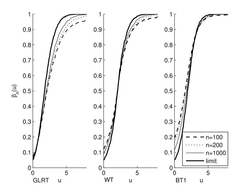
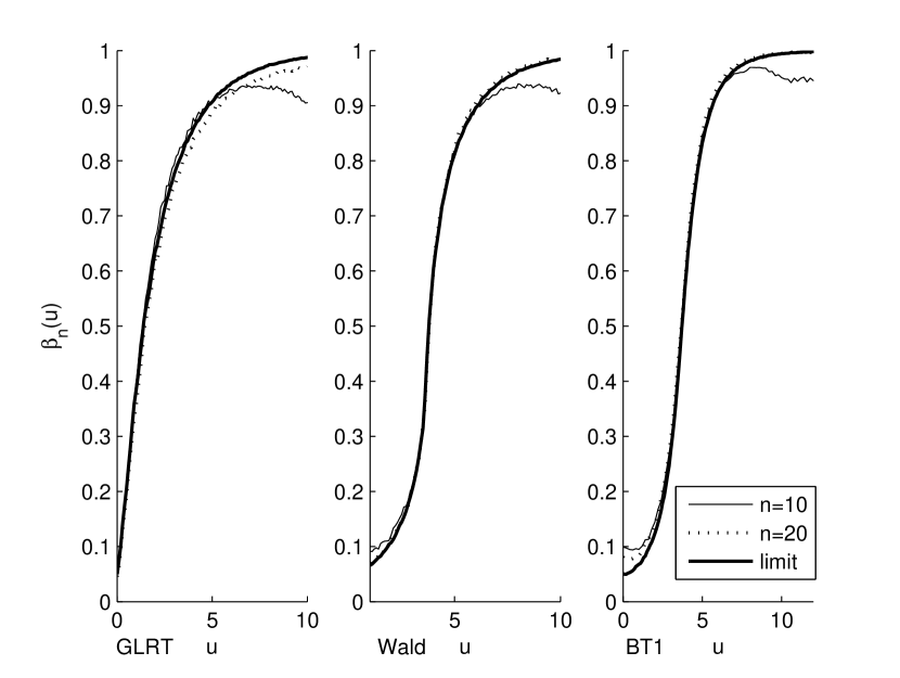
We can see in Figure 3 that, like in the regular case, for the small values of $u$ the power function of the WT converge more slowly than that of the GLRT, but still more quickly than that of the BT1. When $u$ is large, the power function of the BT1 converge more quickly than that of the WT, and the power function of the GLRT converge the most slowly.

 Here Figure 3.  

Since analytic expressions for the power functions of these three tests are not yet available, we compare them with the help of numerical simulations. It is equally interesting to compare them to the Neyman-Pearson Test (N-PT) constructed in the following problem of testing of two simple hypotheses.

Let us fix an alternative $\vartheta_{u_{*}}=\vartheta_{1}+u_{*}\varphi_{n}>\vartheta_{1}$ and consider the hypothesis testing problem

$$\mathscr{H}_{1}\quad :\qquad u=0,$$

$$\mathscr{H}_{2}\quad :\qquad u=u_{*}.$$

The Neyman-Pearson test is

$$\psi_{n}^{*}\left(X^{n}\right)={\mathbb{1}}_{\left\{Z_{n}(u_{*})>d_{\varepsilon}\right\}},$$

where the threshold $d_{\varepsilon}$ is the solution of the equation

$$\mathop{\mathbf{\kern 0.0ptP}}\nolimits\left(Z\left(u_{*}\right)>d_{\varepsilon}\right)=\varepsilon.$$

Recall that $Z_{n}\left(u_{*}\right)\Longrightarrow Z(u_{*})$ and

$$Z\left(u_{*}\right)=\exp\left\{W^{H}\left(u_{*}\right)-\frac{u_{*}^{2H}}{2}\right\}.$$

Hence

$$\mathop{\mathbf{\kern 0.0ptP}}\nolimits\left(Z\left(u_{*}\right)>d_{\varepsilon}\right)=\mathop{\mathbf{\kern 0.0ptP}}\nolimits\left\{W^{H}\left(u_{*}\right)-\frac{u_{*}^{2H}}{2}>\ln d_{\varepsilon}\right\}=\mathop{\mathbf{\kern 0.0ptP}}\nolimits\left(\zeta>\frac{\ln d_{\varepsilon}+\frac{u_{*}^{2H}}{2}}{u_{*}^{H}}\right)$$

and

$$d_{\varepsilon}=e^{z_{\varepsilon}u_{*}^{H}-\frac{u_{*}^{2H}}{2}},$$

where $\zeta\sim\mathcal{N}\left(0,1\right)$ and $\mathop{\mathbf{\kern 0.0ptP}}\nolimits\left(\zeta>z_{\varepsilon}\right)=\varepsilon$.

Of course, it is impossible to use this N-PT in our initial problem, since $u_{*}$ (the value of $u$ under alternative) is unknown. However, as this test is the most powerful in the class $\mathcal{K}_{\varepsilon}$, its power (as function of $u_{*}$) shows an upper bound for power functions of all the tests, and the distances between it and the power functions of the studied tests provide useful information.

To study the likelihood ratio function under the alternative we write

$$Z_{n}(u_{*})=\frac{L\left(\vartheta_{1}+u_{*}\varphi_{n},X^{n}\right)}{L\left(\vartheta_{1},X^{n}\right)}=\left(\frac{L\left(\vartheta_{1}+u_{*}\varphi_{n}-u_{*}\varphi_{n},X^{n}\right)}{L\left(\vartheta_{1}+u_{*}\varphi_{n},X^{n}\right)}\right)^{-1}.$$

So, for the power of the N-PT, we obtain

$$\beta(\psi_{n}^{*},u_{*}) =\mathop{\mathbf{\kern 0.0ptP}}\nolimits_{\vartheta_{1}+u_{*}\varphi_{n}}\left(Z_{n}\left(u_{*}\right)>d_{\varepsilon}\right)$$

$$\longrightarrow\mathop{\mathbf{\kern 0.0ptP}}\nolimits\left(Z\left(-u_{*}\right)^{-1}>d_{\varepsilon}\right)=\mathop{\mathbf{\kern 0.0ptP}}\nolimits\left(\exp\left\{-W^{H}\left(-u_{*}\right)+\frac{u_{*}^{2H}}{2}\right\}>d_{\varepsilon}\right)$$

$$=\mathop{\mathbf{\kern 0.0ptP}}\nolimits\left(\zeta>\frac{\ln d_{\varepsilon}-\frac{u_{*}^{2H}}{2}}{u_{*}^{H}}\right)=\mathop{\mathbf{\kern 0.0ptP}}\nolimits\left(\zeta>z_{\varepsilon}-u_{*}^{H}\right).$$

 Here Figure 4.  

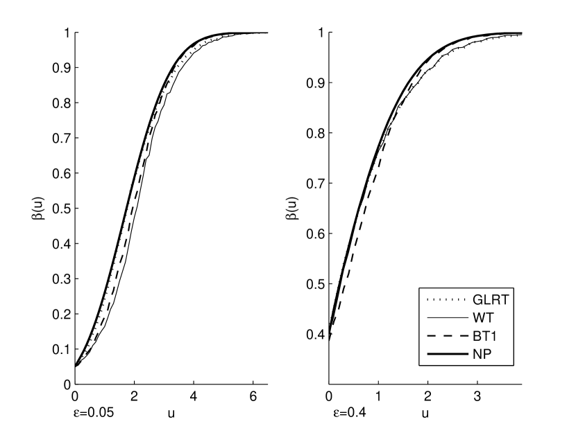
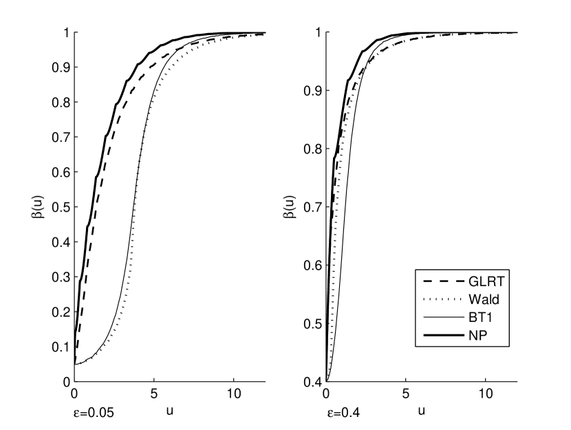
We can see that the limit power function of the GLRT is the closest one to the limit power function of the N-PT. When $u$ is small, the limit power function of the BT1 is lower than that of the GLRT. It becomes closer to that of the N-PT when $u$ increases. At the same time, the limit power function of the WT become the lowest one. Let as also mention that the limit power function of the BT1 arrives faster to $1$ than the others (see Figure 4).

4 Discontinuous intensity

Here we consider a similar hypothesis testing problem in the case of inhomogeneous Poisson processes with discontinuous intensity function. Suppose that the intensity function $\lambda\left(\vartheta,t\right)$, $0\leq t\leq\tau$, of the observed Poisson processes satisfies the following condition.

S. The intensity function $\lambda(\vartheta,t)=\lambda(t-\vartheta)$, where the unknown parameter $\vartheta\in\Theta=\left[\vartheta_{1},b\right)\subset\left(0,\tau\right)$, the function $\lambda(s)$, $s\in\left[-b,\tau-\vartheta_{1}\right]$, is continuously differentiable everywhere except at the point $t_{*}\in\left(-\vartheta_{1},\tau-b\right)$ and this function has a jump at the point $t_{*}$ (and so, the intensity function $\lambda(\vartheta,t)$ has a jump at the point $t=t_{*}+\vartheta\in\left(0,\tau\right)$).

We have to test the hypotheses

$$\mathscr{H}_{1}\quad :\qquad\vartheta=\vartheta_{1},$$

$$\mathscr{H}_{2}\quad :\qquad\vartheta>\vartheta_{1}.$$

We study the same tests as before (GLRT, WT, BT1 and BT2), and our goal is to chose the thresholds so, that these tests belong to the class $\mathcal{K}_{\varepsilon}$. Let us denote $\lambda(t_{*}+)=\lambda_{+}$, $\lambda(t_{*}-)=\lambda_{-}$ and $\rho=\frac{\lambda_{-}}{\lambda_{+}}$. To compare the power functions of the tests, we consider local alternatives which in this problem are given by $\vartheta=\vartheta_{1}+u\varphi_{n}$, $\varphi_{n}=\frac{1}{n\lambda_{+}}$. The initial problem is thus reduced to the following one

$$\mathscr{H}_{1}\quad :\qquad u=0,$$

$$\mathscr{H}_{2}\quad :\qquad u>0.$$

Recall that the normalized likelihood ratio

$$Z_{n}\left(u\right)=\frac{L\left(\vartheta_{1}+u\varphi_{n},X^{n}\right)}{L\left(\vartheta_{1},X^{n}\right)},\qquad u\in\mathbb{U}_{n}^{+}=\bigl{[}0,n\lambda_{+}\left(b-\vartheta_{1}\right)\bigr{)},$$

under the hypothesis $\mathscr{H}_{1}$ converges to the process

$$Z\left(u\right)=\exp\left\{\ln\rho\;x_{*}\left(u\right)-\left(\rho-1\right)u\right\},\qquad u\geq 0,$$

where $(x_{*}\left(u\right),\ u\geq 0)$ is a Poisson process of unit intensity (see [8]).

As we will see below, the limit likelihood ratio under the alternative $\vartheta_{1}+u_{*}\varphi_{n}$, $u_{*}>0$, is

$$Z\left(u,u_{*}\right)=\exp\left\{\ln\rho\;x_{*}\left(u,u_{*}\right)-\left(\rho-1\right)u\right\},\quad u\geq 0,$$

where $(x_{*}\left(u,u_{*}\right),\ u\geq 0)$ is a Poisson process with “switching” intensity function

$$\mu\left(u,u_{*}\right)=\rho\,{\mathbb{1}}_{\left\{u<u_{*}\right\}}+{\mathbb{1}}_{\left\{u\geq u_{*}\right\}},\quad u\geq 0.$$

Note that the limit likelihood ratio of our problem is the likelihood ratio of a similar hypothesis testing problem ($u=0$ against $u>0$) in the case of observations of a Poisson process $(Y\left(t\right),\ t\geq 0)$ with “switching” intensity function $\mu\left(t,u\right)=\rho\,{\mathbb{1}}_{\left\{t<u\right\}}+{\mathbb{1}}_{\left\{t\geq u\right\}}$, $t\geq 0$.

4.1 Weak convergence

The considered tests (GLRT, WT, BT1 and BT2) are functionals of the likelihood function $L\left(\cdot,X^{n}\right)$. As it was shown above, all these tests can be written as functionals of the normalized likelihood ratio $Z_{n}\left(\cdot\right)$. Therefore, as in regular and cusp-type cases, we have to prove the weak convergence of the measures induced by the normalized likelihood ratio under hypothesis (to find the thresholds) and under alternative (to describe the power functions).

Let $\mathscr{D}_{0}$ be the space of functions $z(\cdot)$ on $\mathbb{R}_{+}=\left[0,+\infty\right)$ which do not have discontinuities of the second kind and which are such that $\lim\limits_{v\rightarrow\infty}z(v)=0$. We suppose that the functions $z(\cdot)\in\mathscr{D}_{0}$ are càdlàg, that is, the left limit $z(t-)=\lim\limits_{s\nearrow t}z(s)$ exists and the right limit $z(t+)=\lim\limits_{s\searrow t}z(s)$ exists and equals to $z(t)$. Introduce the distance between two function $z_{1}\left(\cdot\right)$ and $z_{2}\left(\cdot\right)$ as

$$d(z_{1},z_{2})=\inf_{\nu}\Bigl{[}\,\sup_{u\in\mathbb{R}_{+}}\left|z_{1}(u)-z_{2}\bigl{(}\nu(u)\bigr{)}\right|+\sup_{u\in\mathbb{R}_{+}}\left|u-\nu(u)\right|\,\Bigr{]},$$

where the $\inf$ is taken over all monotone continuous one-to-one mappings $\nu:\mathbb{R}_{+}\longrightarrow\mathbb{R}_{+}$. Let us also denote

$$\Delta_{h}(z)=\sup_{u\in\mathbb{R}_{+}}\sup_{\delta}\biggl{\{}\min\Bigl{[}\bigl{|}z(u^{{}^{\prime}})-z(u)\bigr{|},\bigl{|}z(u^{{}^{\prime\prime}})-z(u)\bigr{|}\Bigr{]}\biggr{\}}+\sup_{|u|>1/h}\bigl{|}z(u)\bigr{|},$$

where the second $\sup$ is taken over the intervals $\delta=\left[u^{{}^{\prime}},u^{{}^{\prime\prime}}\right)\,\subseteq\left[u-h,u+h\right)$ such that $u\in\delta$.

Suppose that we have a sequence $\left(Y_{n}\right)_{n\geq 1}$ of stochastic processes $\bigl{(}$with $Y_{n}=(Y_{n}(u),\ u\in\left[0,+\infty\right))\bigr{)}$ and a process $Y_{0}=(Y_{0}(u),\ u\in\left[0,+\infty\right))$ such that the realizations of these processes belong to the space $\mathscr{D}_{0}$. Denote ${\bf Q}_{n}^{(\vartheta)}$ and ${\bf Q}^{(\vartheta)}$ the distributions (which we suppose depending on a parameter $\vartheta\in\Theta$) induced on the measurable space $(\mathscr{D}_{0},\mathcal{B})$ by these processes. Here $\mathcal{B}$ is the Borel $\sigma$-algebra of the metric space $\mathscr{D}_{0}$.

Theorem 1.

If, as $n\rightarrow\infty$, the finite dimensional distributions of the process $Y_{n}$ converge to the finite dimensional distributions of the process $Y_{0}$ uniformly in $\vartheta\in\Theta$ and for any $\delta>0$ we have

$$\lim_{h\rightarrow 0}\,\mathop{\overline{\lim}}\limits_{n\rightarrow\infty}\,\sup_{\vartheta\in\Theta}\,{\bf Q}_{n}^{(\vartheta)}\{\Delta_{h}(Y_{n})>\delta\}=0,$$ (8)

then ${\bf Q}_{n}^{(\vartheta)}\Longrightarrow{\bf Q}^{(\vartheta)}$ uniformly in $\vartheta\in\Theta$ as $n\rightarrow\infty$.

For the proof see [6], Theorem 9.5.2.

Recall that such a weak convergence of the likelihood ratio process $Z_{n}\left(\cdot\right)$ for the discussed model of inhomogeneous Poisson process was already established in [8, Sections 4.4 and 5.4.3] (see as well [9, Chapter 5] for similar results). The proof given there corresponds to the weak convergence in the space $\left(\mathscr{D}_{0},\mathcal{B}\right)$ of $Z_{n}\left(\cdot\right)$ under hypothesis $\mathscr{H}_{1}$. The limit process under the alternative $\vartheta_{1}+u_{*}\varphi_{n}$ is different and we study it below in order to describe the power functions.

Let now ${\bf Q}$ be the measure induced on the measurable space $\left(\mathscr{D}_{0},\mathcal{B}\right)$ by the stochastic processes $(Z\left(u,u_{*}\right),\ u\geq 0)$, and ${\bf Q}_{n}^{(\vartheta)}$ be the measure induced (under the true value $\vartheta$) on the same space by the processes $(Z_{n}\left(u\right),\ u\geq 0)$.

Proposition 5.

Let the condition S be fulfilled. Then, under the alternative $\vartheta_{u_{*}}=\vartheta_{1}+u_{*}\varphi_{n}$, we have the convergence

$${\bf Q}_{n}^{(\vartheta_{u_{*}})}\Longrightarrow{\bf Q}.$$ (9)

The proof is based on several lemmas, where we verify the convergence of the finite-dimensional distributions and the condition (8). As in [8], we follow the main steps of the proof of Ibragimov and Khasminskii [7] of a similar convergence in the case of i.i.d. observations.

Lemma 1.

Let the condition S be fulfilled. Then, under the alternative $\vartheta_{u_{*}}$, the finite-dimensional distributions of the process $(Z_{n}(u),\ u\geq 0)$ converge to those of the process $(Z(u,u_{*}),\ u\geq 0)$.

Proof.

The characteristic function of $\ln Z_{n}\left(u\right)$ is (see [8]):

$$\mathop{\mathbf{\kern 0.0ptE}}\nolimits_{\vartheta_{u_{*}}}\exp\left\{i\mu\ln Z_{n}(u)\right\}$$

$$\qquad=\exp\biggl{[}n\int_{0}^{\tau}\Bigl{(}\exp\Bigl{(}i\mu\ln\frac{\lambda(t-\vartheta_{1}-u\varphi_{n})}{\lambda(t-\vartheta_{1})}\Bigr{)}-1\Bigr{)}\lambda(t-\vartheta_{1}-u_{*}\varphi_{n})\,\mathrm{d}t-$$

$$\qquad\qquad-in\mu\int_{0}^{\tau}\bigl{(}\lambda(t-\vartheta_{1}-u\varphi_{n})-\lambda(t-\vartheta_{1})\bigr{)}\,\mathrm{d}t\biggr{]}$$

$$\qquad=\exp\biggl{(}n\int_{0}^{\tau}A_{n}(u,u_{*},t)\,\mathrm{d}t-in\mu\int_{0}^{\tau}B_{n}(u,u_{*},t)\,\mathrm{d}t\biggr{)}$$

where we denoted

$$A_{n}(u,u_{*},t) =\left[\exp\left(i\mu\ln\frac{\lambda_{u}}{\lambda_{0}}\right)-1-i\mu\ln\frac{\lambda_{u}}{\lambda_{0}}\right]\lambda_{u_{*}},$$

$$B_{n}(u,u_{*},t) =\lambda_{u}-\lambda_{0}-\lambda_{0}\ln\frac{\lambda_{u}}{\lambda_{0}}+\left(\lambda_{0}-\lambda_{u_{*}}\right)\ln\frac{\lambda_{u}}{\lambda_{0}}$$

and $\lambda_{v}=\lambda\left(t-\vartheta_{1}-v\varphi_{n}\right)$ for $v\geq 0$.

We consider two cases: $u\leq u_{*}$ and $u>u_{*}$. Let $u\leq u_{*}$ and $0\leq t\leq t_{*}+\vartheta_{1}$. Then the functions $\lambda_{0},\lambda_{u}$ and $\lambda_{u_{*}}$ are continuously differentiable and, using Taylor expansion, we obtain the estimates

$$\int_{0}^{t_{*}+\vartheta_{1}}\left|A_{n}\left(u,u_{*},t\right)\right|{\rm d}t\leq\frac{Cu^{2}}{n^{2}}\ \>\ \text{and}\ \>\ \int_{0}^{t_{*}+\vartheta_{1}}\left|B_{n}\left(u,u_{*},t\right)\right|{\rm d}t\leq\frac{C\left(u^{2}+uu_{*}\right)}{n^{2}}.$$

Similar estimates hold on the interval $t\in\left[t_{*}+\vartheta_{1}+u_{*}\varphi_{n},\tau\right]$. We have as well the estimates

$$\int_{t_{*}+\vartheta_{1}+u\varphi_{n}}^{t_{*}+\vartheta_{1}+u_{*}\varphi_{n}}\left|A_{n}\left(u,u_{*},t\right)\right|{\rm d}t\leq\frac{Cu^{2}\left(u_{*}-u\right)}{n^{3}}$$

and

$$\int_{t_{*}+\vartheta_{1}+u\varphi_{n}}^{t_{*}+\vartheta_{1}+u_{*}\varphi_{n}}\left|B_{n}\left(u,u_{*},t\right)\right|{\rm d}t\leq\frac{Cu^{2}\left(u_{*}-u\right)}{n^{3}}+\frac{Cu\left(u_{*}-u\right)}{n^{2}}.$$

So, the main contribution comes from the integrals

$$n\int_{t_{*}+\vartheta_{1}}^{t_{*}+\vartheta_{1}+u\varphi_{n}} \left[\exp\left(i\mu\ln\frac{\lambda_{u}}{\lambda_{0}}\right)-1\right]\lambda_{u_{*}}{\rm d}t-i\mu n\int_{t_{*}+\vartheta_{1}}^{t_{*}+\vartheta_{1}+u\varphi_{n}}\left[\lambda_{u}-\lambda_{0}\right]{\rm d}t$$

$$=u\left[\exp\left(i\mu\ln\frac{\lambda_{-}}{\lambda+}\right)-1\right]\frac{\lambda_{-}}{\lambda_{+}}-iu\mu\left[\frac{\lambda_{-}}{\lambda_{+}}-1\right]+o\left(1\right)$$

$$\longrightarrow u\left[\exp\left(i\mu\ln\rho\right)-1\right]\rho-iu\mu\left[\rho-1\right],$$

and we obtain, for $u\leq u_{*}$,

$$\mathop{\mathbf{\kern 0.0ptE}}\nolimits_{\vartheta_{u_{*}}}\exp\left\{i\mu\ln Z_{n}(u)\right\} \longrightarrow\exp\biggl{\{}u\Bigl{(}\bigl{(}\exp\left\{i\mu\ln\rho\right\}-1\bigr{)}\rho-i\mu\left(\rho-1\right)\Bigr{)}\biggr{\}}$$

$$=\mathop{\mathbf{\kern 0.0ptE}}\nolimits\exp\left\{i\mu\ln Z(u,u_{*})\right\}.$$

Now we consider the case $u\geq u_{*}$. As before, we obtain the convergence,

$$n\left(\int_{0}^{t_{*}+\vartheta_{1}}+\int_{t_{*}+\vartheta_{1}+u\varphi_{n}}^{\tau}\right)\bigl{(}\left|A_{n}(u,u_{*},t)\right|+\left|B_{n}(u,u_{*},t)\right|\bigr{)}dt\longrightarrow 0.$$

For the intervals $\left(t_{*}+\vartheta_{1},t_{*}+\vartheta_{1}+u_{*}\varphi_{n}\right)$ and $\bigl{(}t_{*}+\vartheta_{1}+u_{*}\varphi_{n},t_{*}+\vartheta_{1}+u\varphi_{n}\bigr{)}$, we can write

$$n\int_{t_{*}+\vartheta_{1}}^{t_{*}+\vartheta_{1}+u_{*}\varphi_{n}} \bigl{(}A_{n}(u,u_{*},t)-i\mu B_{n}\left(u,u_{*},t\right)\bigr{)}\mathrm{d}t$$

$$\longrightarrow\frac{u_{*}}{\lambda_{+}}\Bigl{(}\exp\Bigl{(}i\mu\ln\frac{\lambda_{-}}{\lambda_{+}}\Bigr{)}-1\Bigr{)}\lambda_{-}-i\mu\bigl{(}\lambda_{-}-\lambda_{+}\bigr{)}\biggr{)}$$

$$=u_{*}\Bigl{(}\bigl{(}\exp\left\{i\mu\ln\rho\right\}-1\bigr{)}\rho-i\mu\left(\rho-1\right)\Bigr{)}$$

and

$$n\int_{t_{*}+\vartheta_{1}+u_{*}\varphi_{n}}^{t_{*}+\vartheta_{1}+u\varphi_{n}} \bigl{(}A_{n}(u,u_{*},t)-i\mu B_{n}\left(u,u_{*},t\right)\bigr{)}\mathrm{d}t$$

$$\longrightarrow\frac{u-u_{*}}{\lambda_{+}}\biggl{(}\Bigl{(}\exp\Bigl{(}i\mu\ln\frac{\lambda_{-}}{\lambda_{+}}\Bigr{)}-1\Bigr{)}\lambda_{+}-i\mu\bigl{(}\lambda_{-}-\lambda_{+}\bigr{)}\biggr{)}.$$

So, for $u>u_{*}$, we get

$$\mathop{\mathbf{\kern 0.0ptE}}\nolimits_{\vartheta_{u_{*}}}\exp\left\{i\mu\ln Z_{n}(u)\right\} \longrightarrow\exp\biggl{\{}u_{*}\Bigl{(}\bigl{(}\exp\left\{i\mu\ln\rho\right\}-1\bigr{)}\rho-i\mu\left(\rho-1\right)\Bigr{)}$$

$$\qquad\qquad+(u-u_{*})\Bigl{(}\exp\left\{i\mu\ln\rho\right\}-1-i\mu\left(\rho-1\right)\Bigr{)}\biggr{\}}$$

$$=\mathop{\mathbf{\kern 0.0ptE}}\nolimits\exp\left\{i\mu\ln Z(u,u_{*})\right\}.$$

Therefore the one-dimensional distributions of the stochastic process $Z_{n}\left(\cdot\right)$ converge to those of $Z\left(\cdot,u_{*}\right)$.

The convergence of arbitrary finite-dimensional distributions of $Z_{n}\left(\cdot\right)$ to those of $Z\left(\cdot,u_{*}\right)$ can be proved in a similar manner. For example, in the case of two-dimensional distributions we can write (for $u_{1}<u_{2}<u_{*}$)

$$\mathop{\mathbf{\kern 0.0ptE}}\nolimits_{\vartheta_{u_{*}}} \exp\bigl{\{}i\mu_{1}\ln Z_{n}(u_{1})+i\mu_{2}\ln Z_{n}(u_{2})\bigr{\}}$$

$$\longrightarrow\exp\biggl{\{}(u_{2}-u_{1})\Bigl{[}\bigl{(}\exp\left\{i\mu_{2}\ln\rho\right\}-1\bigr{)}\rho-i\mu_{2}(\rho-1)\Bigr{]}$$

$$\qquad\qquad+u_{1}\Bigl{[}\Bigl{(}\exp\bigl{\{}i\,(\mu_{1}+\mu_{2})\ln\rho\bigr{\}}-1\Bigr{)}\rho-i\,(\mu_{1}+\mu_{2})\,(\rho-1)\Bigr{]}\biggr{\}}$$

$$=\mathop{\mathbf{\kern 0.0ptE}}\nolimits\exp\bigl{\{}i\mu_{1}\ln Z(u_{1},u_{*})+i\mu_{2}\ln Z(u_{2},u_{*})\bigr{\}}.$$

So, the lemma is proved. ∎

Further, we can write

$$Z_{n}(u)=Z_{n}(u_{*})\;\widetilde{Z}_{n}(u),$$

where

$$\widetilde{Z}_{n}(u)=\frac{\mathrm{d}\mathop{\mathbf{\kern 0.0ptP}}\nolimits_{\vartheta_{1}+u\varphi_{n}}\hfill}{\mathrm{d}\mathop{\mathbf{\kern 0.0ptP}}\nolimits_{\vartheta_{1}+u_{*}\varphi_{n}}\hfill}\qquad\text{and}\qquad Z_{n}(u_{*})=\frac{\mathrm{d}\mathop{\mathbf{\kern 0.0ptP}}\nolimits_{\vartheta_{1}+u_{*}\varphi_{n}}\hfill}{\mathrm{d}\mathop{\mathbf{\kern 0.0ptP}}\nolimits_{\vartheta_{1}}\hfill}.$$

Note that $Z_{n}\left(u_{*}\right)$ does not depend of $u$ and we have the convergence (under the alternative $\vartheta_{u_{*}}=\vartheta_{1}+u\varphi_{n}$)

$$Z_{n}\left(u_{*}\right)\Longrightarrow Z_{*}\left(u_{*}\right)=\exp\left\{\ln\rho\;x_{\rho}\left(u_{*}\right)-u_{*}\left(\rho-1\right)\right\},$$ (10)

where $(x_{\rho}\left(u\right),\ u\geq 0)$ is a Poisson process of intensity $\rho$. Therefore, to prove (9), it is sufficient to study the convergence of the measures induced by the stochastic process $(\widetilde{Z}_{n}(u),\ u\geq 0)$.

Lemma 2.

Let the conditions S be fulfilled. Then there exists a constant $C>0$, such that

$$\mathop{\mathbf{\kern 0.0ptE}}\nolimits_{\vartheta_{1}+u_{*}\varphi_{n}}\bigl{|}\widetilde{Z}_{n}^{1/2}(u_{1})-\widetilde{Z}_{n}^{1/2}(u_{2})\bigr{|}^{2}\leq C\left|u_{1}-u_{2}\right|$$ (11)

for all $u_{*},u_{1},u_{2}\in\mathbb{U}_{n}^{+}$.

Proof.

According to [9, Lemma 1.1.5], we have (for $v_{1}>v_{2}>0$)

$$\mathop{\mathbf{\kern 0.0ptE}}\nolimits_{\vartheta_{1}+u_{*}\varphi_{n}}\bigl{|}\widetilde{Z}_{n}^{1/2}(u_{1})-\widetilde{Z}_{n}^{1/2}(u_{2})\bigr{|}^{2}$$

$$\ \,\leq\int_{0}^{n\tau}\left(\frac{\lambda^{1/2}(t-\vartheta_{1}-u_{1}\varphi_{n})}{\lambda^{1/2}(t-\vartheta_{1}-u_{*}\varphi_{n})}-\frac{\lambda^{1/2}(t-\vartheta_{1}-u_{2}\varphi_{n})}{\lambda^{1/2}(t-\vartheta_{1}-u_{*}\varphi_{n})}\,\right)^{2}\lambda(t-\vartheta_{1}-u_{*}\varphi_{n})\,\mathrm{d}t$$

$$\ \,=n\int_{0}^{\tau}\bigl{(}\lambda^{1/2}(t-\vartheta_{1}-u_{1}\varphi_{n})-\lambda^{1/2}(t-\vartheta_{1}-u_{2}\varphi_{n})\,\bigr{)}^{2}\,\mathrm{d}t$$

$$\ \,=n\left(\int_{0}^{t_{*}+u_{2}\varphi_{n}}+\int_{t_{*}+u_{2}\varphi_{n}}^{t_{*}+u_{1}\varphi_{n}}+\int_{t_{*}+u_{1}\varphi_{n}}^{\tau}\right)\bigl{(}\lambda_{u_{1}}^{1/2}-\lambda_{u_{2}}^{1/2}\,\bigr{)}^{2}\,\mathrm{d}t$$

$$\ \,=n(I_{1}+I_{2}+I_{3})$$

with obvious notations.

As the functions $\lambda_{u_{1}}$ and $\lambda_{u_{2}}$ are continuously differentiable on the intervals $\left[0,t_{*}+u_{2}\varphi_{n}\right]$ and $\left[t_{*}+u_{1}\varphi_{n},\tau\right]$, we can write

$$\lambda^{\frac{1}{2}}\left(\vartheta_{1}+u_{1}\varphi_{n},t\right)-\lambda^{\frac{1}{2}}\left(\vartheta_{1}+u_{2}\varphi_{n},t\right)=\frac{\left(u_{1}-u_{2}\right)\varphi_{n}}{2}\,\frac{\dot{\lambda}\left(\vartheta_{v},t\right)}{\lambda^{\frac{1}{2}}\left(\vartheta_{v},t\right)}\,,$$

where $v$ is some intermediate point between $u_{1}$ and $u_{2}$. Therefore

$$n\left(I_{1}+I_{3}\right) \leq n\varphi_{n}^{2}\frac{(u_{1}-u_{2})^{2}}{4}\left(\int_{0}^{t_{*}+u_{2}\varphi_{n}}+\int_{t_{*}+u_{1}\varphi_{n}}^{\tau}\right)\frac{\dot{\lambda}\left(\vartheta_{v},t\right)^{2}}{\lambda\left(\vartheta_{v},t\right)}\,\mathrm{d}t$$

$$\leq\frac{C}{n\lambda_{+}^{2}}\left|u_{1}-u_{2}\right|^{2}\leq{C}\left|u_{1}-u_{2}\right|$$

where we took into account the inequality $\left|u_{1}-u_{2}\right|\leq Cn$.

Since the function $\lambda$ is bounded, we have the estimate

$$nI_{2}\leq n\frac{\left|u_{1}-u_{2}\right|}{n\lambda_{+}}C=\frac{C}{\lambda_{+}}\left|u_{1}-u_{2}\right|,$$

and so the inequality (11) holds with some constant $C>0$. ∎

Lemma 3.

Let the condition S be fulfilled. Then there exists a constant $k^{*}>0$ such that

$$\mathop{\mathbf{\kern 0.0ptE}}\nolimits_{\vartheta_{1}+u_{*}\varphi_{n}}\widetilde{Z}_{n}^{1/2}(u)\leq\exp\bigl{\{}-k^{*}\left|u-u_{*}\right|\bigr{\}}$$ (12)

for all $u^{*},u\in\mathbb{U}_{n}^{+}$.

Proof.

According to [9, Lemma 1.1.5], we have

$$\mathop{\mathbf{\kern 0.0ptE}}\nolimits_{\vartheta_{1}+u_{*}\varphi_{n}}\widetilde{Z}_{n}^{1/2}(u)$$

$$\qquad=\exp\Bigl{\{}-\frac{n}{2}\int_{0}^{\tau}\Bigl{(}\frac{\lambda^{1/2}(t-\vartheta_{1}-u\varphi_{n})}{\lambda^{1/2}(t-\vartheta_{1}-u_{*}\varphi_{n})}-1\,\Bigr{)}^{2}\,\lambda(t-\vartheta_{1}-u_{*}\varphi_{n})\,\mathrm{d}t\Bigr{\}}$$

$$\qquad=\exp\Biggl{\{}-\frac{n}{2}\,\int_{0}^{\tau}\Bigl{(}\lambda^{1/2}\bigl{(}t-\vartheta_{1}-u\varphi_{n}\bigr{)}-\lambda^{1/2}(t-\vartheta_{1}-u_{*}\varphi_{n})\,\Bigr{)}^{2}\,\mathrm{d}t\Biggr{\}}$$

$$\qquad=\exp\left\{-\frac{n}{2}\,F_{n}(u,u_{*})\right\}$$

with an obvious notation.

Let us consider separately the cases $u\in D=\left\{v:\;\left|v-u_{*}\right|<\delta n\lambda_{+}\right\}$ and $u\in D^{c}=\left\{v:\;\left|v-u_{*}\right|\geq\delta n\lambda_{+}\right\}$. Here $\delta$ is some positive constant which will be chosen later. For simplicity we suppose that $u>u_{*}$.

For the values $u\in D$ we have

$$nF_{n}(u,u_{*}) \geq n\int_{t_{*}+\vartheta_{1}+u_{*}\varphi_{n}}^{t_{*}+\vartheta_{1}+u\varphi_{n}}\left[\lambda^{1/2}\bigl{(}t-\vartheta_{1}-u\varphi_{n}\bigr{)}-\lambda^{1/2}(t-\vartheta_{1}-u_{*}\varphi_{n})\right]^{2}\,\mathrm{d}t$$

$$\geq\frac{\left|u-u_{*}\right|}{\lambda_{+}}\inf_{t_{*}+u_{*}\varphi_{n}\leq s\leq t_{*}+u\varphi_{n}}\left[\lambda^{1/2}\bigl{(}s-u\varphi_{n}\bigr{)}-\lambda^{1/2}(s-u_{*}\varphi_{n})\right]^{2}$$

$$\geq\frac{\left|u-u_{*}\right|}{2\lambda_{+}}\left(\sqrt{\lambda_{-}}-\sqrt{\lambda_{+}}\right)^{2}=\frac{\left|u-u_{*}\right|}{2}\left(\sqrt{\rho}-1\right)^{2}$$

for sufficiently small $\delta$.

Further, note that for any $\nu>0$ we have

$$g\left(\nu\right)=\inf_{\left|s-s_{0}\right|>\nu}\int_{0}^{\tau}\left[\sqrt{\lambda\left(t-\vartheta_{1}-s\right)}-\sqrt{\lambda\left(t-\vartheta_{1}-s_{0}\right)}\right]^{2}{\rm d}t>0.$$

Indeed, if $g\left(\nu\right)=0$ then for some $s_{*}$ we have $\lambda\left(t-\vartheta_{1}-s_{*}\right)=\lambda\left(t-\vartheta_{1}-s_{0}\right)$ for all $t\in\left[0,\tau\right]$, but this equality for discontinuous $\lambda\left(\cdot\right)$ and all $t$ is impossible. Hence, for the values $u\in D^{c}$ we have

$$nF_{n}\left(u,u_{*}\right)\geq ng\left(\delta\right)\geq\frac{g\left(\delta\right)\left|u-u_{*}\right|}{C}$$

where we took into account the inequality $\left|u-u_{*}\right|\leq Cn$.

So, the inequality (12) is proved. ∎

The presented estimates (11), (12) and Lemma 1 allow us to finish the proof following the same lines as it was done in [8], Section 5.4.3.

4.2 GLRT

The GLRT is based on the statistic

$$Q_{n}\left(X^{n}\right)=\sup_{\vartheta\geq\vartheta_{1}}L\left(\vartheta,\vartheta_{1},X^{n}\right)=\max\left[L\left(\hat{\vartheta}_{n}+,\vartheta_{1},X^{n}\right),\,L\left(\hat{\vartheta}_{n}-,\vartheta_{1},X^{n}\right)\right]$$

(where $\hat{\vartheta}_{n}$ is the MLE) and is of the form

$$\hat{\psi}_{n}\left(X^{n}\right)={\mathbb{1}}_{\left\{Q_{n}\left(X^{n}\right)>h_{\varepsilon}\right\}}.$$

The threshold $h_{\varepsilon}$ is defined with the help of the convergence (under hypothesis $\mathscr{H}_{1}$)

$$Q_{n}\left(X^{n}\right)=\sup_{u\in\mathbb{U}_{n}^{+}}Z_{n}\left(u\right)\Longrightarrow\sup_{u>0}Z\left(u\right)=\hat{Z}.$$

Hence $h_{\varepsilon}=h_{\varepsilon}\left(\rho\right)$ is solution of the equation

$$\mathop{\mathbf{\kern 0.0ptP}}\nolimits\left\{\hat{Z}>h_{\varepsilon}\right\}=\varepsilon.$$

Let us fix an alternative $\vartheta_{u_{*}}=\vartheta_{1}+u_{*}\varphi_{n}$, $u_{*}>0$. Then for the power function we have

$$\beta\left(\hat{\psi}_{n},u_{*}\right)=\mathop{\mathbf{\kern 0.0ptE}}\nolimits_{\vartheta_{u_{*}}}\hat{\psi}_{n}\left(X^{n}\right) =\mathop{\mathbf{\kern 0.0ptP}}\nolimits_{\vartheta_{u_{*}}}\left\{\sup_{u>0}Z_{n}\left(u\right)>h_{\varepsilon}\right\}$$

$$\longrightarrow\mathop{\mathbf{\kern 0.0ptP}}\nolimits\left\{\sup_{u>0}Z\left(u,u_{*}\right)>h_{\varepsilon}\right\}.$$

Putting $Y\left(u\right)=\ln Z\left(u,u_{*}\right)=\ln\rho\,x_{*}\left(u,u_{*}\right)-\left(\rho-1\right)u$, we can write

$$\sup_{u>0}Y(u)=\max\left(\sup_{0<u<u_{*}}Y\left(u\right),\>Y\left(u_{*}\right)+\sup_{u\geq u_{*}}\left[Y\left(u\right)-Y\left(u_{*}\right)\right]\right).$$

Note that the Poisson process $\tilde{x}\left(v\right)=x_{*}\left(u_{*}+v,u_{*}\right)-x_{*}\left(u_{*},u_{*}\right)$, $v\geq 0$, is independent from $(x_{*}\left(u,u_{*}\right),\ 0\leq u\leq u_{*})$. Hence we can write the following representation of the limit power function:

$$\beta\left(\hat{\psi}_{n},u_{*}\right)\longrightarrow\mathop{\mathbf{\kern 0.0ptP}}\nolimits\left\{\max\left(\sup_{0<u<u_{*}}Z_{*}\left(u\right),\>Z_{*}\left(u_{*}\right)\,\tilde{Z}\right)>h_{\varepsilon}\right\},$$

where the random variable $\tilde{Z}=\sup\limits_{v\geq 0}\exp\left\{{\ln\rho\,\tilde{x}_{*}\left(v\right)}-\left(\rho-1\right)v\right\}$ is independent from $(Z_{*}\left(u\right),\ 0\leq u\leq u_{*})$, and the process $Z_{*}\left(\cdot\right)$ is defined as in (10). Let us note that this expression is useful for numerical simulation of the power function. It simplifies the calculations since the simulated values of $\tilde{Z}$ can be used many times for different values of $u_{*}$.

4.3 Wald test

The Wald test is based on the MLE $\hat{\vartheta}_{n}$. We already know that

$$\varphi_{n}^{-1}\left(\hat{\vartheta}_{n}-\vartheta_{1}\right)\Longrightarrow\hat{u},$$

where $\hat{u}$ is defined by the equation

$$\max\left[Z\left(\hat{u}+\right),Z\left(\hat{u}-\right)\right]=\sup_{u>0}Z\left(u\right).$$

The Wald test is

$$\psi_{n}^{\circ}\left(X^{n}\right)={\mathbb{1}}_{\left\{\varphi_{n}^{-1}\left(\hat{\vartheta}_{n}-\vartheta_{1}\right)>g_{\varepsilon}\right\}},$$

where the threshold $g_{\varepsilon}=g_{\varepsilon}\left(\rho\right)$ is solution of the equation

$$\mathop{\mathbf{\kern 0.0ptP}}\nolimits\left\{\hat{u}>g_{\varepsilon}\right\}=\varepsilon.$$

For the power function we have (below $\vartheta_{u_{*}}=\vartheta_{1}+u_{*}\varphi_{n}$)

$$\beta\left(\psi_{n}^{\circ},u_{*}\right) =\mathop{\mathbf{\kern 0.0ptE}}\nolimits_{\vartheta_{u_{*}}}\psi_{n}^{\circ}\left(X^{n}\right)=\mathop{\mathbf{\kern 0.0ptP}}\nolimits_{\vartheta_{u_{*}}}\left\{\varphi_{n}^{-1}\left(\hat{\vartheta}_{n}-\vartheta_{1}\right)>h_{\varepsilon}\right\}$$

$$=\mathop{\mathbf{\kern 0.0ptP}}\nolimits_{\vartheta_{u_{*}}}\left\{\sup_{\varphi_{n}^{-1}\left(\theta-\vartheta_{1}\right)>h_{\varepsilon}}L\left(\theta,X^{n}\right)>\sup_{\varphi_{n}^{-1}\left(\theta-\vartheta_{1}\right)\leq h_{\varepsilon}}L\left(\theta,X^{n}\right)\right\}$$

$$=\mathop{\mathbf{\kern 0.0ptP}}\nolimits_{\vartheta_{u_{*}}}\left\{\sup_{\varphi_{n}^{-1}\left(\theta-\vartheta_{1}\right)>h_{\varepsilon}}\frac{L\left(\theta,X^{n}\right)}{L\left(\vartheta_{1},X^{n}\right)}>\sup_{\varphi_{n}^{-1}\left(\theta-\vartheta_{1}\right)\leq h_{\varepsilon}}\frac{L\left(\theta,X^{n}\right)}{L\left(\vartheta_{1},X^{n}\right)}\right\}$$

$$=\mathop{\mathbf{\kern 0.0ptP}}\nolimits_{\vartheta_{u_{*}}}\left\{\sup_{u>h_{\varepsilon}}Z_{n}\left(u\right)>\sup_{u\leq h_{\varepsilon}}Z_{n}\left(u\right)\right\}$$

$$\longrightarrow\mathop{\mathbf{\kern 0.0ptP}}\nolimits\left\{\sup_{u>h_{\varepsilon}}Z\left(u,u_{*}\right)>\sup_{u\leq h_{\varepsilon}}Z\left(u,u_{*}\right)\right\}=\mathop{\mathbf{\kern 0.0ptP}}\nolimits\left\{\hat{u}^{*}>h_{\varepsilon}\right\},$$

where the random variable $\hat{u}^{*}$ is defined by the equation

$$\max\left[Z\left(\hat{u}^{*}+,u\right),Z\left(\hat{u}^{*}-,u\right)\right]=\sup_{u\geq 0}Z\left(u,u_{*}\right).$$

Let us note, that we can also give another representation of the power function using the limit (under the alternative $\vartheta_{u_{*}}$) of the normalized likelihood ratio $L(\vartheta_{u_{*}}+u\varphi_{n},\vartheta_{u_{*}},X^{n})$, $u\geq-u_{*}$. This limit is the stochastic process $(Z^{\star}\left(u\right),\ u\geq-u_{*})$ defined by

$$Z^{\star}\left(u\right)=\begin{cases}\exp\bigl{\{}\ln\rho\;x_{*}\left(u\right)-\left(\rho-1\right)u\bigr{\}}&\text{if }u\geq 0,\vphantom{\Big{(}}\\ \exp\bigl{\{}-\ln\rho\;x_{\rho}\bigl{(}(-u)-\bigr{)}-\left(\rho-1\right)u\bigr{\}}&\text{if }-u_{*}\leq u\leq 0\vphantom{\Big{(}},\end{cases}$$

where $(x_{*}\left(u\right),\ u\geq 0)$ and $(x_{\rho}\left(u\right),\ u\geq 0)$ are Poisson processes of unit intensity and of intensity $\rho$ respectively. Note that in [8] this limit was established for a fixed value $\vartheta$ but, taking into account Section 4.1, it clearly holds for “moving” value $\vartheta_{u_{*}}$. Note also that the positive real axis part $(Z^{\star}\left(u\right),\ u\geq 0)$ of the process $Z^{\star}(\cdot)$ is nothing but the process $Z\left(\cdot\right)$.

Now, we have

$$\beta\left(\psi_{n}^{\circ},u_{*}\right)=\mathop{\mathbf{\kern 0.0ptE}}\nolimits_{\vartheta_{u_{*}}}\psi_{n}^{\circ}\left(X^{n}\right) =\mathop{\mathbf{\kern 0.0ptP}}\nolimits_{\vartheta_{u_{*}}}\left\{\varphi_{n}^{-1}\left(\hat{\vartheta}_{n}-\vartheta_{u_{*}}\right)+u_{*}>h_{\varepsilon}\right\}$$

$$\longrightarrow\mathop{\mathbf{\kern 0.0ptP}}\nolimits\left\{\hat{u}_{*}>h_{\varepsilon}-u_{*}\right\}$$

where $\hat{u}_{*}$ is defined by the equation

$$\max\left[Z^{\star}\left(\hat{u}_{*}+\right),Z^{\star}\left(\hat{u}_{*}-\right)\right]=\sup_{u\geq-u_{*}}Z^{\star}\left(u\right).$$

4.4 Bayes tests

Suppose that the parameter $\vartheta$ is a random variable with known probability density $p\left(\theta\right)$, $\vartheta_{1}\leq\theta<b$. This function is supposed to be continuous and positive.

We consider two Bayes tests. The first one is based on the Bayes estimator, while the second one is based on the averaged likelihood ratio.

The first test, which we call BT1, is similar to WT, but is based on the Bayes estimator (BE) $\tilde{\vartheta}_{n}$ rather than on the MLE:

$$\tilde{\psi}_{n}\left(X^{n}\right)={\mathbb{1}}_{\left\{\varphi_{n}^{-1}\left(\tilde{\vartheta}_{n}-\vartheta_{1}\right)>k_{\varepsilon}\right\}},\qquad\tilde{\vartheta}_{n}=\frac{\int_{\vartheta_{1}}^{b}\theta p\left(\theta\right)L\left(\theta,\vartheta_{1},X^{n}\right){\rm d}\theta}{\int_{\vartheta_{1}}^{b}\theta L\left(\theta,\vartheta_{1},X^{n}\right){\rm d}\theta}.$$

The properties of the likelihood ratio established in Lemmas 1–3 allow us to justify the limit

$$\mathop{\mathbf{\kern 0.0ptE}}\nolimits_{\vartheta_{1}}\tilde{\psi}_{n}\left(X^{n}\right)\longrightarrow\mathop{\mathbf{\kern 0.0ptP}}\nolimits\left\{\tilde{u}>k_{\varepsilon}\right\},\qquad\tilde{u}=\frac{\int_{0}^{\infty}vZ\left(v\right){\rm d}v}{\int_{0}^{\infty}Z\left(v\right){\rm d}v}.$$

The proof follows from the general results concerning the Bayes estimators described in [7] (see as well [8]).

For the power function, using the convergence (under the alternative $\vartheta_{u_{*}}$) of the process $Z_{n}\left(\cdot\right)$ to the process $Z\left(\cdot,u_{*}\right)$, we obtain

$$\beta\left(\tilde{\psi}_{n},u_{*}\right)=\mathop{\mathbf{\kern 0.0ptP}}\nolimits_{\vartheta_{u_{*}}}\left\{\varphi_{n}^{-1}\left(\tilde{\vartheta}_{n}-\vartheta_{1}\right)>k_{\varepsilon}\right\}\longrightarrow\mathop{\mathbf{\kern 0.0ptP}}\nolimits\left\{\frac{\int_{0}^{\infty}vZ\left(v,u_{*}\right){\rm d}v}{\int_{0}^{\infty}Z\left(v,u_{*}\right){\rm d}v}>k_{\varepsilon}\right\}.$$

Let us note, that we can also give another representation of the limit power function using the process $Z^{\star}\left(\cdot\right)$. We have the convergence (under the alternative $\vartheta_{u_{*}}$)

$$\varphi_{n}^{-1}\left(\tilde{\vartheta}_{n}-\vartheta_{1}\right)=\varphi_{n}^{-1}\left(\tilde{\vartheta}_{n}-\vartheta_{u_{*}}\right)+u_{*}\Longrightarrow\frac{\int_{-u_{*}}^{\infty}vZ^{\star}\left(v\right){\rm d}v}{\int_{-u_{*}}^{\infty}Z^{\star}\left(v\right){\rm d}v}+u_{*}.$$

Hence

$$\beta\left(\tilde{\psi}_{n},u_{*}\right)\longrightarrow\mathop{\mathbf{\kern 0.0ptP}}\nolimits\left\{\frac{\int_{-u_{*}}^{\infty}vZ^{\star}\left(v\right){\rm d}v}{\int_{-u_{*}}^{\infty}Z^{\star}\left(v\right){\rm d}v}>k_{\varepsilon}-u_{*}\right\}.$$

The second test, which we call BT2, is the test which minimizes the mean error of the second kind. We have

$$\varphi_{n}^{-1}\tilde{L}\left(X^{n}\right)=\varphi_{n}^{-1}\int_{\vartheta_{1}}^{b}p\left(\theta\right)\frac{L\left(\theta,X^{n}\right)}{L\left(\vartheta_{1},X^{n}\right)}\,{\rm d}\theta\Longrightarrow p\left(\vartheta_{1}\right)\int_{0}^{\infty}Z\left(v\right)\;{\rm d}v.$$

Hence the test

$$\tilde{\psi}_{n}^{\star}\left(X^{n}\right)={\mathbb{1}}_{\left\{R_{n}>m_{\varepsilon}\right\}},\qquad R_{n}=\frac{\tilde{L}\left(X^{n}\right)}{\varphi_{n}\;p\left(\vartheta_{1}\right)}\,,$$

with threshold $m_{\varepsilon}$ satisfying the equation

$$\mathop{\mathbf{\kern 0.0ptP}}\nolimits\left\{\int_{0}^{\infty}Z\left(v\right){\rm d}v>m_{\varepsilon}\right\}=\varepsilon$$

belongs to the class $\mathcal{K}_{\varepsilon}$ and minimizes the mean error of the second kind.

4.5 Simulations

We consider $n$ independent realizations $X_{j}=(X_{j}(t),\ t\in\left[0,4\right])$, $j=1,\ldots,n$, of a Poisson process of intensity function

$$\lambda(t,\vartheta)=\lambda(t-\vartheta)=3-2\cos^{2}(t-\vartheta){\mathbb{1}}_{\left\{t\geq\vartheta\right\}},\qquad 0\leq t\leq 4.$$

We take $\vartheta_{1}=3$ and $b=4$, and therefore $\lambda_{+}=1$, $\lambda_{-}=3$ and $\rho=\frac{\lambda_{-}}{\lambda_{+}}=3$. The log-likelihood ratio is

$$\ln Z_{n}(u) =\sum_{j=1}^{n}\int_{3}^{3+u/n}\ln\frac{3}{3-2\cos^{2}(t-3)}\,{\rm d}X_{j}(t)$$

$$\qquad+\sum_{j=1}^{n}\int_{3+u/n}^{4}\ln\frac{3-2\cos^{2}(t-3-u/n)}{3-2\cos^{2}(t-3)}\,{\rm d}X_{j}(t)$$

$$\qquad-u-\frac{n}{2}\sin\bigl{(}2\bigr{)}+\frac{n}{2}\sin\bigl{(}2(1-u/n)\bigr{)}.$$

Recall that in this case the limit (under $\mathscr{H}_{1}$) of the likelihood ratio is

$$Z\left(u\right)=\exp\left\{\ln 3\;x_{*}\left(u\right)-2u\right\},$$

where $(x_{*}\left(u\right),\ u\geq 0)$ is a Poisson process of unit intensity. A realization of this limit likelihood ratio $\bigl{(}$or, more precisely, of the logarithm of its two-sided version $Z^{\star}\left(\cdot\right)\bigr{)}$ and its zoom are given in Figure 5.

 Here Figure 5.  

Using this limit we obtain the threshold $h_{\varepsilon}$ of the GLRT as solution of the equation

$$\mathop{\mathbf{\kern 0.0ptP}}\nolimits\left\{\sup_{u>0}Z(u)>h_{\varepsilon}\right\}=\varepsilon.$$

It is convenient for simulations to transform the limit process as follows:

$$\exp\left[\ln 3\left(x_{*}\left(u\right)-\frac{2}{\ln 3}u\right)\right]=\exp\left\{\ln 3\left[\Pi\left(\frac{2}{\ln 3}u\right)-\frac{2}{\ln 3}u\right]\right\}$$

where $\Pi\left(\cdot\right)$ is a Poisson process of intensity $\gamma=\frac{\ln 3}{2}<1$. Hence, the threshold $h_{\varepsilon}$ is determined by the equation

$$\mathop{\mathbf{\kern 0.0ptP}}\nolimits\left\{\sup_{t>0}\left[\Pi\left(t\right)-t\right]>\frac{\ln h_{\varepsilon}}{\ln 3}\right\}=\varepsilon.$$

The distribution of $\sup\limits_{t>0}\left[\Pi\left(t\right)-t\right]$ is given by the well-known formula

$$\mathop{\mathbf{\kern 0.0ptP}}\nolimits\left\{\sup_{t>0}\left[\Pi\left(t\right)-t\right]\geq x\right\}=\sum_{m>x}\frac{(m-x)^{m}}{m!}(\gamma e^{-\gamma})^{m}e^{\gamma x}(1-\gamma)$$

obtained by Pyke in [15].

Note that there is equally an analytic expression for the distribution of the random variable $\hat{t}=\mathop{\rm argmax}\limits_{t\geq 0}\left[\Pi\left(t\right)-t\right]$. This expression was obtained by Pflug in [14] and is given by

$$\mathop{\mathbf{\kern 0.0ptP}}\nolimits\left\{\hat{t}<z\right\}=\mathop{\mathbf{\kern 0.0ptP}}\nolimits\left\{\sum_{k=1}^{\nu}\eta_{k}<z\right\},$$

where $\left\{\eta_{k}\right\}_{k\in\mathbb{N}^{*}}$ is an i.i.d. sequence with common distribution

$$\mathop{\mathbf{\kern 0.0ptP}}\nolimits\left\{\eta_{k}\leq x\right\}=\frac{1}{\gamma}\left[1-(1-\gamma)e^{-\gamma x}\sum_{j=0}^{[x]-1}\frac{(\gamma x)^{j}}{j\,!}-e^{-\gamma x}\frac{(\gamma x)^{[x]}}{[x]\,!}\right],$$

$\nu$ is a random variable independent of $\eta_{k}$, $k\in\mathbb{N}^{*}$, and distributed according to geometric law

$$\mathop{\mathbf{\kern 0.0ptP}}\nolimits\left\{\nu=i\right\}=(1-\gamma)\gamma^{i},\quad i\in\mathbb{N},$$

and we use the convention $\sum_{k=1}^{0}\eta_{k}=0$. Now, for the threshold $g_{\varepsilon}$ of the WT we can write

$$\mathop{\mathbf{\kern 0.0ptP}}\nolimits\left\{\hat{u}>g_{\varepsilon}\right\}=\mathop{\mathbf{\kern 0.0ptP}}\nolimits\left\{\mathop{\rm argmax}\limits_{t\geq 0}\left[\Pi\left(t\right)-t\right]>\frac{\ln 3}{2}g_{\varepsilon}\right\}=\varepsilon.$$

However, the numerical solution of this equation is not easy, and it is simpler to obtain the threshold $g_{\varepsilon}$ by Monte Carlo simulations.

The thresholds are presented in Table 2.

$\varepsilon$	0.01	0.05	0.10	0.20	0.40	0.50
$\ln h_{\varepsilon}$	4.242	2.607	1.922	1.120	0.573	0.191
$g_{\varepsilon}$	5.990	3.556	2.078	1.045	0.329	0.099
$k_{\varepsilon}$	6.669	3.937	2.983	2.132	1.402	1.196

Table 2: Thresholds of GLRT, WT and BT1

 Here Figure 6.  

It is interesting to compare the studied tests with the Neyman-Pearson test (N-PT) corresponding to a fixed value $u_{*}$ of $u$. Of course, it is impossible to use this N-PT in our initial problem, since $u_{*}$ (the value of $u$ under alternative) is unknown. Nevertheless, its power (as function of $u_{*}$) shows an upper bound for power functions of all the tests, and the distances between it and the power functions of studied tests provide an important information. Let us fix some value $u_{*}>0$ and introduce the N-PT

$$\psi_{n}^{*}\left(X^{n}\right)={\mathbb{1}}_{\left\{Z_{n}(u_{*})>d_{\varepsilon}\right\}}+q_{\varepsilon}{\mathbb{1}}_{\left\{Z_{n}(u_{*})=d_{\varepsilon}\right\}},$$

where $d_{\varepsilon}$ and $q_{\varepsilon}$ are solutions of the equation

$$\mathop{\mathbf{\kern 0.0ptP}}\nolimits\left(Z\left(u_{*}\right)>d_{\varepsilon}\right)+q_{\varepsilon}\mathop{\mathbf{\kern 0.0ptP}}\nolimits\left(Z\left(u_{*}\right)=d_{\varepsilon}\right)=\varepsilon.$$

Denoting $D_{\varepsilon}=\left(\ln d_{\varepsilon}+(\rho-1)u_{*}\right)/\ln\rho$, we can rewrite this equation as

$$\mathop{\mathbf{\kern 0.0ptP}}\nolimits\left(x_{*}(u_{*})>D_{\varepsilon}\right)+q_{\varepsilon}\mathop{\mathbf{\kern 0.0ptP}}\nolimits\left(x_{*}(u_{*})=D_{\varepsilon}\right)=\varepsilon.$$

Here $x_{*}\left(u_{*}\right)$ is a Poisson random variable with parameter $u_{*}$, and so the quantities $D_{\varepsilon}$ and $q_{\varepsilon}$ can be computed numerically.

A similar calculation yields the limit power of the N-PT:

$$\beta\left(\psi_{n}^{*},u_{*}\right)\longrightarrow\mathop{\mathbf{\kern 0.0ptP}}\nolimits\left(x_{*}(u_{*},u_{*})>D_{\varepsilon}\right)+q_{\varepsilon}\mathop{\mathbf{\kern 0.0ptP}}\nolimits\left(x_{*}(u_{*},u_{*})=D_{\varepsilon}\right).$$

where $x_{*}\left(u_{*},u_{*}\right)$ is a Poisson random variable with parameter $\rho u_{*}$.

 Here Figure 7.  

The results of simulations are presented in Figure 7 for two cases: $\varepsilon=0.05$ and $\varepsilon=0.4$. In both cases the limit power function of the GLRT is the closest one to the limit power of the N-PT, and the limit power function of the BT1 arrives faster to $1$ than the others.

5 Acknowledgements

This study was partially supported by Russian Science Foundation (research project No. 14-49-00079). The authors thank the Referee for helpful comments.

Figure 1: A realization of $Z_{n}(\cdot)$ with $\lambda\left(\vartheta,t\right)=2-\left|t-1.5\right|^{0.4}$ and $n=1000$

Figure 2: A realization of $Z_{n}(\cdot)$ with $\lambda\left(\vartheta,t\right)=0.5+\left|t-1.5\right|^{0.4}$ and $n=1000$

Figure 3: Power functions of GLRT, WT and BT1 in cusp case with $\lambda\left(\vartheta,t\right)=2-\left|t-\vartheta\right|^{0.4}$

Figure 4: Comparison of limit power functions in cusp case with $\lambda\left(\vartheta,t\right)=2-\left|t-\vartheta\right|^{0.4}$

Figure 5: A realization of $\ln Z^{\star}(\cdot)$

Figure 6: Power functions of GLRT, WT and BT1 in discontinuous case with $\rho=3$

Figure 7: Comparison of limit power functions in discontinuous case with $\rho=3$

References

- [1] Dachian S., Estimation of cusp location by Poisson observations. Stat. Inference Stoch. Process., 2003, 6, 1, 1–14.
- [2] Dachian S. and Kutoyants Yu. A., Hypotheses testing : Poisson versus stress-release, J. Statist. Plan. Inference, 2009, 139, 1668–1684.
- [3] Dachian S., Kutoyants Yu. A. and L. Yang., On hypothises testing for Poisson processes. Regular case. submitted, 2014.
- [4] Daley, Vere-Jones, D., An Introduction to the Theory of Point Processes, v. 1, 2nd edit., Springer, N.Y. 2003.
- [5] Fierro, R. and Tapia, A., Testing homogeneity for Poisson processes. Rev. Colombiana Estadíst., 2011, 34, 421–432.
- [6] Gikhman, I.I. and Skorohod, A.V., Introduction to the Theory of Random Processes. Saunders, Philadelphia, 1969.
- [7] Ibragimov, I.A. and Hasminskii, R.Z., Statistical Estimation. Asymptotic Theory, Springer, N. Y., 1981.
- [8] Kutoyants, Yu.A., Parameter Estimation for Stochastic Processes, Armenian Academy of Sciences, Yerevan, 1980 (in Russian), translation of revised version, Heldermann, Berlin, 1984.
- [9] Kutoyants, Yu. A., Statistical Inference for Spatial Poisson Processes, Lect. Notes Statist. 134, Springer, N. Y., 1998.
- [10] Kutoyants, Yu. A., Introduction to Statistics of Poisson Processes, to appear, 2014.
- [11] Le Cam, L., Asymptotic Methods in Statistical Decision Theory. Springer, N. Y., 1986.
- [12] Léger, C. and Wolfson, D. B., Hypothesis testing for a non-homogeneous Poisson process. Stoch. Models, 1987, 3, 439-455.
- [13] Lehmann, E. and Romano, J., Testing Statistical Hypotheses, Springer, Heidelberg, 2005.
- [14] Pflug, G. C., On an argmax-distribution connected to the Poisson process, Proceedings of the Fifth Prague Conference on Asymtotic Statistics, P.Mandl and M. Huskova eds, 1993, 123–130.
- [15] Pyke, R., The supremum and infimum of the Poisson process, Ann. Math. Statist., 1959, 30, 568–576.