Estimation of exponential-polynomial distribution by holonomic gradient descent

Abstract

We study holonomic gradient decent for maximum likelihood estimation of exponential-polynomial distribution, whose density is the exponential function of a polynomial in the random variable. We first consider the case that the support of the distribution is the set of positive reals. We show that the maximum likelihood estimate (MLE) can be easily computed by the holonomic gradient descent, even though the normalizing constant of this family does not have a closed-form expression and discuss determination of the degree of the polynomial based on the score test statistic. Then we present extensions to the whole real line and to the bivariate distribution on the positive orthant.

Keywords and phrases:  algebraic statistics, bivariate distribution, score test.

1 Introduction

Exponential distribution and the truncated normal distribution have been frequently used for positive continuous random variables (e.g., Chapter 19 and Section 13.10 of [7], [14]). Generalizing these two cases, in this paper we consider fitting a density function which is the exponential function of a polynomial in the random variable. For simplicity we first study the case of a positive random variable. For $x>0$, consider the following density

$$f(x;\theta_{1},\dots,\theta_{d})=\frac{1}{A(\theta_{1},\dots,\theta_{d})}\exp(\theta_{1}x+\dots+\theta_{d}x^{d}),\qquad\theta_{d}<0,$$ (1)

where

$$A(\theta_{1},\dots,\theta_{d})=\int_{0}^{\infty}\exp(\theta_{1}x+\dots+\theta_{d}x^{d})\mbox{$\mathrm{d}$}x$$ (2)

is the normalizing constant of this density. In the following we write $A_{d}(\bm{\theta})=A(\theta_{1},\dots,\theta_{d})$. We call (1) the exponential-polynomial distribution of order $d$. Although it is a natural generalization of the exponential ($d=1$) and the truncated normal distribution ($d=2$), it has been rarely used in statistics. One reason is that $A_{d}(\bm{\theta})$ can not be written in a closed form. Another reason may be that the tail of the distribution is light because of the term $\theta_{d}x^{d}$, $\theta_{d}<0$. However by having this term, we can allow arbitrary values of $\theta_{1},\dots,\theta_{d-1}$ and have a flexible family of distributions.

Concerning the treatment of the normalizing constant, recently in [11] we proposed a new method, called the holonomic gradient decent (HGD), for evaluating the normalizing constant of the exponential family and for computing MLE. As in the subsequent works ([5], [13]), we show that HGD works well also for the case of exponential-polynomial distribution.

When we fit (1) to a given sample, the natural question we face is the determination of the order $d$ of the model. The exponential-polynomial model has a special structure that the model of order $d-1$ with $\theta_{d}=0$ and $\theta_{d-1}<0$ is the boundary of the model of order $d$ with $\theta_{d}<0$. In regular hypothesis testing problems or model selection problems, a submodel is assumed to be a smooth manifold of a smaller dimension in the interior of a larger model. Hence we need to adapt model selection procedures to this non-regular case. We propose selection of $d$ by a score test.

The organization of this paper is as follows. In Sections 2–4 we study exponential-polynomial distribution over the set of positive reals. In Section 2 we derive a differential equation satisfied by $A_{d}(\bm{\theta})$ and use the differential equation to compute MLE. In Section 3 we discuss how to determine the order $d$ of the model by a score test. In Section 4 we present results of some numerical experiments. In Section 5 we extend the exponential-polynomial distribution to the whole real line and in Section 6 we study a bivariate exponential-polynomial distribution. We end the paper with some discussions on further extension of the model in Section 7.

2 Maximum likelihood estimation via holonomic gradient descent

Given a sample $\bm{x}=(x_{1},\dots,x_{n})$ of size $n$, $(1/n)$ times the log-likelihood function is written as

$$\bar{l}(\bm{\theta};\bm{x})=\theta_{1}\bar{x}+\theta_{2}\bar{x^{2}}+\dots+\theta_{d}\bar{x^{d}}-\psi(\bm{\theta}),\qquad\psi(\bm{\theta})=\log A_{d}(\bm{\theta}),$$ (3)

where $\bar{x^{m}}=\sum_{i=1}^{n}x_{i}^{m}/n$, $m=1,\dots,d$. Let $\partial_{m}=\frac{\partial}{\partial\theta_{m}}$ denote the differentiation with respect to $\theta_{m}$. In maximizing $\bar{l}$ with respect to $\bm{\theta}$, we want to compute its gradient

$$\nabla\bar{l}=\begin{bmatrix}\partial_{1}\bar{l}\\ \vdots\\ \partial_{d}\bar{l}\end{bmatrix}=\begin{bmatrix}\bar{x}\\ \vdots\\ \bar{x^{d}}\end{bmatrix}-\begin{bmatrix}\partial_{1}\psi\\ \vdots\\ \partial_{d}\psi\end{bmatrix},\quad\partial_{m}\psi(\bm{\theta})=\frac{\partial_{m}A_{d}(\bm{\theta})}{A_{d}(\bm{\theta})}$$

and its Hessian matrix

$$H(\bar{l})(\bm{\theta})=-H(\psi)(\bm{\theta})=-\begin{bmatrix}\partial_{1}^{2}\psi&\cdots&\partial_{1}\partial_{d}\psi\\ \vdots&\cdots&\vdots\\ \partial_{d}\partial_{1}\psi&\cdots&\partial_{d}^{2}\psi\end{bmatrix},\quad\partial_{l}\partial_{m}\psi(\bm{\theta})=\frac{\partial_{l}\partial_{m}A_{d}(\bm{\theta})}{A_{d}(\bm{\theta})}-\frac{\partial_{l}A_{d}(\bm{\theta})}{A_{d}(\bm{\theta})}\frac{\partial_{m}A_{d}(\bm{\theta})}{A_{d}(\bm{\theta})}.$$

Note that $I(\bm{\theta})=H(\psi)(\bm{\theta})$ is the Fisher information matrix for $\bm{\theta}$.

In (2) we can interchange the integration and the differentiation by elements of $\bm{\theta}$ as many time as needed. Hence derivatives of $A_{d}(\bm{\theta})$ can be evaluated by numerical integration. However it is cumbersome to perform numerical integration for the derivatives at every $\bm{\theta}$. The holonomic gradient decent allows us to compute $A_{d}(\bm{\theta})$ and its derivatives at any point by numerically solving a differential equation from those at an initial point $\bm{\theta}=\bm{\theta}^{0}$. The fact that $A_{d}(\bm{\theta})$ is a holonomic function (cf. Section 1 and Appendix of [11], Chapter 6 of [6], [15]) guarantees the existence of a differential equation with polynomial coefficients satisfied by $A_{d}(\bm{\theta})$. Also, for our problem there is a convenient initial point (see (9) below), where $A_{d}(\bm{\theta})$ and its derivatives have a closed-form expression. Hence by using the holonomic gradient descent, we do not need any numerical integration for our problem.

Differentiating (2) by $\theta_{1}$ we have

$$\partial_{1}A_{d}(\bm{\theta})=\int_{0}^{\infty}x\exp(\theta_{1}x+\dots+\theta_{d}x^{d})\mbox{$\mathrm{d}$}x.$$

Repeating this $i$ times we have

$$\partial_{1}^{i}A_{d}(\bm{\theta})=\int_{0}^{\infty}x^{i}\exp(\theta_{1}x+\dots+\theta_{d}x^{d})\mbox{$\mathrm{d}$}x.$$ (4)

However the right-hand side is also equal to $\partial_{i}A(\bm{\theta})$. Hence the following relation holds.

$$\partial_{i}A_{d}(\bm{\theta})=\partial_{1}^{i}A_{d}(\bm{\theta}).$$ (5)

In general, for any higher-order mixed derivative $\partial_{1}^{j_{1}}\dots\partial_{d}^{j_{d}}A(\bm{\theta})$ we have the relation

$$\partial_{1}^{j_{1}}\dots\partial_{d}^{j_{d}}A_{d}(\bm{\theta})=\partial_{1}^{j_{1}+2j_{2}+\dots+dj_{d}}A_{d}(\bm{\theta}).$$

Hence all mixed derivatives reduce to the derivatives of $A_{d}(\bm{\theta})$ with respect to $\theta_{1}$. It follows that for numerical purposes we only need to keep in memory the derivatives of $A_{d}(\bm{\theta})$ with respect to $\theta_{1}$.

Now as a relation among the derivatives of $A_{d}(\bm{\theta})$ with respect to $\theta_{1}$, we have the following theorem.

Theorem 2.1.

$A_{d}(\bm{\theta})$ satisfies the following differential equation

$$(\theta_{1}+2\theta_{2}\partial_{1}+3\theta_{3}\partial_{1}^{2}+\dots+d\theta_{d}\partial_{1}^{d-1})A_{d}(\bm{\theta})=-1.$$ (6)

Proof.

$$-1 =\big{[}\exp(\theta_{1}x+\dots+\theta_{d}x^{d})\big{]}_{0}^{\infty}$$

$$=\int_{0}^{\infty}\partial_{x}\exp(\theta_{1}x+\dots+\theta_{d}x^{d})\;\mbox{$\mathrm{d}$}x$$

$$=\int_{0}^{\infty}(\theta_{1}+2\theta_{2}x+3\theta_{3}x^{2}+\dots+d\theta_{d}x^{d-1})\exp(\theta_{1}x+\dots+\theta_{d}x^{d})\mbox{$\mathrm{d}$}x$$

$$=(\theta_{1}+2\theta_{2}\partial_{1}+3\theta_{3}\partial_{1}^{2}+\dots+d\theta_{d}\partial_{1}^{d-1})A_{d}(\bm{\theta}).\hskip 56.9055pt\text{(by \eqref{eq:partial1i})}$$

∎

By (6), $\partial_{1}^{d-1}A_{d}(\bm{\theta})$ is written in terms of lower-order derivatives as

$$\partial_{1}^{d-1}A_{d}(\bm{\theta})={-\frac{1}{d\theta_{d}}\left\{1+\Big{(}\theta_{1}+2\theta_{2}\partial_{1}+3\theta_{3}\partial_{1}^{2}+\dots+(d-1)\theta_{d-1}\partial_{1}^{d-2}\Big{)}A_{d}(\bm{\theta})\right\}.}$$ (7)

Recursively differentiating this by $\theta_{1}$ we see that all higher-order derivatives $\partial_{1}^{m}A_{d}(\bm{\theta})$, $m\geq d-1$, can be written in terms of the elements of a vector

$$F(\bm{\theta})=[A_{d}(\bm{\theta}),\partial_{1}A_{d}(\bm{\theta}),\dots,\partial_{1}^{d-2}A_{d}(\bm{\theta})]^{\mathsf{T}},$$

where ^T denotes the transpose of a vector or a matrix. If $F(\bm{\theta})$ can be evaluated at any point $\bm{\theta}$, then by (5) we can evaluate the gradient of $A_{d}$ and hence can compute MLE of the exponential-polynomial distribution.

The directional derivative of $F(\bm{\theta})$ in the direction $\bm{h}=(h_{1},\dots,h_{d})$ is written as

$$\frac{\partial}{\partial s}F(\bm{\theta}+s\bm{h})=\sum_{j=1}^{d}h_{j}\partial_{j}F(\bm{\theta}+s\bm{h})=\sum_{j=1}^{d}h_{j}\partial_{1}^{j}F(\bm{\theta}+s\bm{h})=\sum_{j=1}^{d}h_{j}\begin{bmatrix}\partial_{1}^{j}A_{d}(\bm{\theta}+s\bm{h})\\ \partial_{1}^{j+1}A_{d}(\bm{\theta}+s\bm{h})\\ \vdots\\ \partial_{1}^{j+d-2}A_{d}(\bm{\theta}+s\bm{h})\end{bmatrix}.$$ (8)

If we differentiate (7) recursively, we obtain $(d-1)\times(d-1)$ matrices (called the Pfaffian matrices) $R_{j}$, $j=1,\dots,d$, with rational function elements such that the vector on the right-hand side of (8) is written as

$$\begin{bmatrix}\partial_{1}^{j}A_{d}(\bm{\theta}+s\bm{h})\\ \partial_{1}^{j+1}A_{d}(\bm{\theta}+s\bm{h})\\ \vdots\\ \partial_{1}^{j+d-2}A_{d}(\bm{\theta}+s\bm{h})\end{bmatrix}=R_{j}(\bm{\theta}+s\bm{h})F(\bm{\theta}+s\bm{h}).$$

Then the equation

$$\frac{\partial}{\partial s}F(\bm{\theta}+s\bm{h})=\sum_{j=1}^{d}h_{j}R_{j}(\bm{\theta}+s\bm{h})F(\bm{\theta}+s\bm{h})$$

can be solved by standard ODE solvers, such as the Runge-Kutta method, when an appropriate initial point $\bm{\theta}_{0}$ and $F(\bm{\theta}_{0})$ are given. This is the procedure of HGD introduced in [11].

As a convenient initial point consider $\bm{\theta}^{0}=(0,0,\dots,0,-c)$, $c>0$. Then

$$\partial_{1}^{m}A_{d}(\bm{\theta}^{0})=\int_{0}^{\infty}x^{m}\exp(-cx^{d})\mbox{$\mathrm{d}$}x=\frac{1}{d}c^{-(1+m)/d}\Gamma\big{(}\frac{1+m}{d}\big{)},\qquad m\geq 0,$$ (9)

which do not need numerical integration.

Remark 2.2.

Nobuki Takayama pointed out that $A_{d}$ satisfies an incomplete $A$-hypergeometric system introduced in [12]. In particular Theorem 2.2 of [12] gives a basic result on incomplete $A$-hypergeometric systems for a class of integrals including our $A_{d}$. See also Section 6.12 of [6].

In summary, we have shown that the evaluation of $A_{d}(\bm{\theta})$ and the maximization of the likelihood function can be performed by using only a standard solver for an ordinary differential equation. As we see in Section 4 this method works quite well in practice.

3 Determination of the degree of the model

When we fit the exponential-polynomial distribution in (1) to a given sample, we need to determine the order $d$ of the model. Suppose that we are fitting the model with order $d-1$ and wondering whether a model of order $d$ fits better. One difficulty with (7) is that it becomes unstable as $\theta_{d}\rightarrow 0$, i.e., the differential equation (6) has a singularity at $\theta_{d}=0$. Hence if the data really come from the model of order $d-1$, the estimation of the model of order $d$ by our method tends to be unstable.

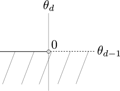
Figure 1: Model of order $d-1$ within the model of order $d$

We can understand this problem by considering the parameter spaces of order $d-1$ and $d$. Let $\Omega_{d}=\{(\theta_{1},\dots,\theta_{d})\mid\theta_{d}<0\}\subset{\mathbb{R}}^{d}$ denote the parameter space of the model of order $d$. $\Omega_{d}$ is an open subset of ${\mathbb{R}}^{d}$. Now $\Omega_{d-1}=\{(\theta_{1},\dots,\theta_{d-1},0)\mid\theta_{d-1}<0\}$ considered as a subset of ${\mathbb{R}}^{d}$ is on the boundary of $\Omega_{d}$. See Figure 1. In $(\theta_{d-1},\theta_{d})$-plane, $\Omega_{d}$ is the lower half open plane and $\Omega_{d-1}$ the left half open $\theta_{d-1}$-axis $\{(\theta_{d-1},0)\mid\theta_{d-1}<0\}$. Since $A_{d}(\theta_{1},\dots,\theta_{d-1},0)$ is finite for $\theta_{d-1}<0$, MLE may not exist in the open set $\Omega_{d}$ with positive probability. For each $d$, consider $\Omega_{1},\dots,\Omega_{d}$ as subsets of ${\mathbb{R}}^{d}$ and let $\bar{\Omega}_{d}=\Omega_{1}\cup\cdots\cup\Omega_{d}$. Since $A_{d}(\bm{\theta})<\infty$ if and only if the last non-zero element of $\bm{\theta}$ is negative, we have $\bar{\Omega}_{d}=\{\bm{\theta}\mid A(\bm{\theta})<\infty\}$. $\psi_{d}(\bm{\theta})={\log}A_{d}(\bm{\theta})$ is strictly convex on $\bar{\Omega}_{d}$ and approaches $+\infty$ as $\bm{\theta}$ approaches the open boundary of $\bar{\Omega}_{d}$, such as the right half open $\theta_{d-1}$-axis $\{(\theta_{d-1},0)\mid\theta_{d-1}>0\}$ in Figure 1. Hence MLE always exists in $\bar{\Omega}_{d}$ but may not fall on $\Omega_{d}$.

We now consider the hypothesis testing problem:

$$H_{0}:\bm{\theta}\in\Omega_{d-1}\ \ \text{v.s.}\ \ H_{1}:\bm{\theta}\in\Omega_{d}.$$ (10)

If $H_{0}$ is true let $\bm{\theta}^{*}\in\Omega_{d-1}$ denote the true parameter vector and let $\hat{\bm{\theta}}_{d-1}=(\hat{\theta}_{1},\dots,\hat{\theta}_{d-1},0)$, $\hat{\theta}_{d-1}\leq 0$, denote the MLE under $H_{0}$. $\hat{\bm{\theta}}_{d-1}$ may belong to $\Omega_{k},k<d-1$. However as $n\rightarrow\infty$, $\hat{\bm{\theta}}_{d-1}$ converges to $\bm{\theta}^{*}$ in probability.

The MLE $\hat{\bm{\theta}}_{d-1}$ under $H_{0}$ satisfies

$$\partial_{j}\bar{l}(\hat{\bm{\theta}}_{d-1};\bm{x})=0,\qquad j=1,\dots,d-1.$$

Note that $\bar{l}(\hat{\bm{\theta}}_{d-1}+s\bm{h};\bm{x})$ is strictly concave in $s\geq 0$ for any $\bm{h}=(h_{1},\dots,h_{d})$, $h_{d}<0$, i.e., on any half line emanating from $\hat{\bm{\theta}}_{d-1}$ into $\Omega_{d}$. Hence on this half line, $\bar{l}(\hat{\bm{\theta}}_{d-1}{+s\bm{h}};\bm{x})$ is maximized at $s=0$ if and only if

$$\ 0\geq\frac{\partial}{\partial s}\bar{l}(\hat{\bm{\theta}}_{d-1}+s\bm{h};\bm{x})|_{s=0}=\sum_{j=1}^{d}h_{j}\partial_{j}\bar{l}(\hat{\bm{\theta}}_{d-1};\bm{x})=h_{d}\partial_{d}\bar{l}(\hat{\bm{\theta}}_{d-1};\bm{x})\\ \Leftrightarrow\ \partial_{d}\bar{l}(\hat{\bm{\theta}}_{d-1};\bm{x})\geq 0.$$

Note that the right-hand side does not depend on $\bm{h}$. Hence MLE does not exist on $\Omega_{d}$ if and only if $\partial_{d}\bar{l}(\hat{\bm{\theta}}_{d-1};\bm{x})\geq 0$. In this case $\hat{\bm{\theta}}_{d-1}$ is the MLE over $\bar{\Omega}_{d}$.

Let the $d\times d$ Fisher information matrix $I(\bm{\theta})=H(\psi)(\bm{\theta})$ be partitioned as

$$I(\bm{\theta})=\begin{bmatrix}I_{d-1,d-1}(\bm{\theta})&I_{d-1,d}(\bm{\theta})\\ I_{d,d-1}(\bm{\theta})&I_{dd}(\bm{\theta})\end{bmatrix},$$

where $I_{dd}$ is a scalar. $I(\bm{\theta})$ is non-singular, since the score functions $\partial_{m}\bar{l}(\bm{\theta};\bm{x})=\bar{x^{m}}-\partial_{m}\psi(\bm{\theta})$, $m=1,\dots,d$, are moments and linearly independent for any $\bm{\theta}$. Note that we put a comma between two subscripts when the subscripts are more complicated. Define

$$I_{dd\cdot 1,\dots,d-1}(\bm{\theta})=I_{dd}(\bm{\theta})-I_{d,d-1}(\bm{\theta})I_{d-1,d-1}(\bm{\theta})^{-1}I_{d-1,d}(\bm{\theta}).$$

In the standard case, where $\Omega_{d-1}$ is in the interior of $\Omega_{d}$, the two-sided test based on

$$\frac{n(\partial_{d}\bar{l}(\hat{\bm{\theta}}_{d-1};\bm{x}))^{2}}{I_{dd\cdot 1,\dots,d-1}(\hat{\bm{\theta}}_{d-1})}$$

is the score test for (10) (e.g., Section 7.7 of [10]). In our case $\Omega_{d-1}$ is the boundary of $\Omega_{d}$ and we reject $H_{0}$ if $\partial_{d}\bar{l}(\hat{\bm{\theta}}_{d-1};\bm{x})$ is negative and its absolute value is too large. However, from the form of the log-likelihood function in (3), the asymptotic null distribution $\partial_{d}\bar{l}(\hat{\bm{\theta}}_{d-1};\bm{x})$ is the same as in the standard case, i.e.,

$$\sqrt{n}\partial_{d}\bar{l}(\hat{\bm{\theta}}_{d-1};\bm{x})\stackrel{{\scriptstyle d}}{{\rightarrow}}\mbox{$\mathrm{N}$}(0,I_{dd\cdot 1,\dots,d-1}(\bm{\theta}^{*}))\qquad(n\rightarrow\infty).$$

Since $\hat{\bm{\theta}}_{d-1}$ converges to $\bm{\theta}^{*}$, we propose the following score test statistic

$$T_{d-1}=\frac{\sqrt{n}\partial_{d}\bar{l}(\hat{\bm{\theta}}_{d-1};\bm{x})}{\sqrt{I_{dd\cdot 1,\dots,d-1}(\hat{\bm{\theta}}_{d-1})}}.$$ (11)

Let $z_{\alpha}$ denote the upper $\alpha$ quantile of $\mbox{$\mathrm{N}$}(0,1)$. Given a significance level $\alpha<1/2$, we can reject $H_{0}$ if $T_{d-1}\leq-z_{\alpha}$, in view of the convergence in distribution

$$T_{d-1}\stackrel{{\scriptstyle d}}{{\rightarrow}}\mbox{$\mathrm{N}$}(0,1)\qquad(n\rightarrow\infty).$$ (12)

4 Numerical experiments for the case of positive real line

We present results of some numerical experiments to show that MLE by HGD works well. We also check the asymptotic approximation in (12).

4.1 Performance of MLE by the holonomic gradient descent

The asymptotic distribution of MLE $\hat{\bm{\theta}}_{d}$ is

$$\sqrt{n}(\hat{\bm{\theta}}_{d}-\bm{\theta}^{*})\stackrel{{\scriptstyle d}}{{\rightarrow}}\mbox{$\mathrm{N}$}_{d}(0,I(\bm{\theta}^{*})^{-1})\qquad(n\rightarrow\infty),$$

where $I(\bm{\theta}^{*})$ is the Fisher information matrix at the true parameter $\bm{\theta}^{*}$. We assume that $\bm{\theta}^{*}$ is an element of $\Omega_{d}$ (hence not an element of $\bar{\Omega}_{d}\setminus\Omega_{d}$). Write

$$p_{i}=\frac{\sqrt{n}(\hat{\theta}_{i}-\theta_{i}^{*})}{\sqrt{I^{-1}_{ii}(\bm{\theta}^{*})}},\qquad i=1,2,\dots,d,$$ (13)

where $I^{-1}_{ii}(\bm{\theta}^{*})$ denotes the $(i,i)$-component of $I(\bm{\theta}^{*})^{-1}$. Then

$$p_{i}\stackrel{{\scriptstyle d}}{{\rightarrow}}\mbox{$\mathrm{N}$}(0,1)\qquad(n\rightarrow\infty).$$ (14)

Thus in our experiments we fix the true parameter $\bm{\theta}^{*}$, apply our method to simulated samples many times and we check the convergence of the empirical distribution of $p_{i}$ to $\mbox{$\mathrm{N}$}(0,1)$.

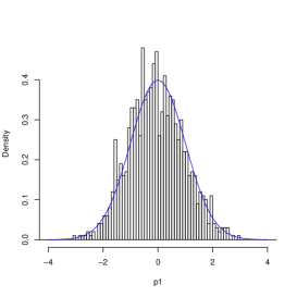
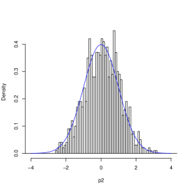
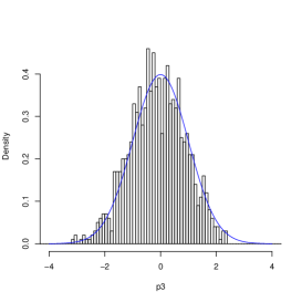
Figure 2: Histogram of $p_{i}$, $i=1,2,3$ (from left to right) and density of $\mathrm{N}$(0,1) for $d=3$

We present simulation results for $d=3$ in (1). We set $\bm{\theta}^{*}=(-1,3,-2)$. In the experiment we used $n=1000$ and iterated computing MLE $1000$ times (i.e. the replication size is 1000). Computation of MLE quickly converged in each iteration. The histogram of $p_{i}$ is given in Figure 2. The curved lines in these figures are the density function of $\mbox{$\mathrm{N}$}(0,1)$. By comparing the histogram and the curved line we see that MLE by HGD works well.

4.2 Asymptotic approximation for score tests

We check the asymptotic approximation in (12) in the case of $d=3,4$. For $d=3$ we set $\bm{\theta}^{*}=(3,-2,0)$. The histograms of $T_{2}$ and $T_{3}$ are shown in Figure 3 (left to right). Again the asymptotic approximation works as expected.

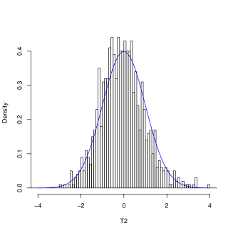
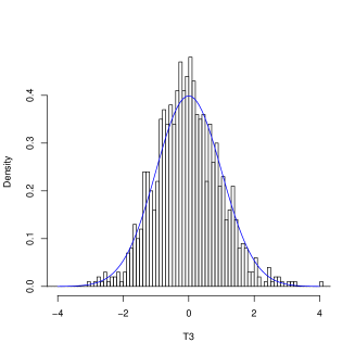
Figure 3: Histogram of $T_{d-1}$ and the density of $\mbox{$\mathrm{N}$}(0,1)$ for $d=3,4$

5 Exponential-polynomial distribution on the whole real line

In this section we extend the result of previous sections to the following density for the whole real line ${\mathbb{R}}^{1}$. Consider the density function

$$f(x;\theta_{1},\dots,\theta_{2d})=\frac{1}{A(\theta_{1},\dots,\theta_{2d})}\exp(\theta_{1}x+\dots+\theta_{2d}x^{2d}),\qquad\theta_{2d}<0,$$ (15)

where

$$A(\theta_{1},\dots,\theta_{2d})=\int_{-\infty}^{\infty}\exp(\theta_{1}x+\dots+\theta_{2d}x^{2d})\mbox{$\mathrm{d}$}x$$ (16)

is the normalizing constant of this density. In following we write $A_{2d}(\bm{\theta})=A(\theta_{1},\dots,\theta_{2d})$.

5.1 Maximum likelihood estimation for the whole line

The holonomic gradient decent is almost the same as in the previous sections. We have

$$\partial_{1}^{i}A_{2d}(\bm{\theta})=\int_{{-\infty}}^{\infty}x^{i}\exp(\theta_{1}x+\dots+\theta_{2d}x^{2d})\mbox{$\mathrm{d}$}x,\quad i=1,2,\dots.$$

Also $\partial_{i}A_{2d}(\bm{\theta})=\partial_{1}^{i}A_{2d}(\bm{\theta}).$ In general $\partial_{1}^{j_{1}}\dots\partial_{d}^{j_{d}}A_{2d}(\bm{\theta})=\partial_{1}^{j_{1}+2j_{2}+\dots+dj_{d}}A_{2d}(\bm{\theta}).$ Hence all mixed derivatives reduce to the derivatives of $A_{2d}(\bm{\theta})$ with respect to $\theta_{1}$. It follows that for numerical purposes we only need to keep in memory the derivatives of $A_{2d}(\bm{\theta})$ with respect to $\theta_{1}$.

Now as a relation among the derivatives of $A_{2d}(\bm{\theta})$ with respect to $\theta_{1}$ we have the following theorem.

Theorem 5.1.

$A_{2d}(\bm{\theta})$ satisfies the following differential equation

$$(\theta_{1}+2\theta_{2}\partial_{1}+3\theta_{3}\partial_{1}^{2}+\dots+2d\theta_{{2d}}\partial_{1}^{2d-1})A_{2d}(\bm{\theta})=0.$$ (17)

Proof is omitted since it almost the same as the proof of Theorem 2.1, by noting

$$0=\big{[}\exp(\theta_{1}x+\dots+\theta_{2d}x^{2d})\big{]}_{-\infty}^{\infty}.$$

By (17), $\partial_{1}^{2d-1}A_{2d}(\bm{\theta})$ is written in terms of lower-order derivatives as

$$\partial_{1}^{2d-1}A_{2d}(\bm{\theta})=-\frac{1}{2d\theta_{2d}}(\theta_{1}+2\theta_{2}\partial_{1}+3\theta_{3}\partial_{1}^{2}+\dots+(2d-1)\theta_{2d-1}\partial_{1}^{2d-2})A_{2d}(\bm{\theta}).$$

Recursively differentiating this by $\theta_{1}$ all higher-order derivatives $\partial_{1}^{m}A_{2d}(\bm{\theta})$, $m\geq 2d-1$, can be easily written in terms of $A_{2d}(\bm{\theta}),\partial_{1}A_{2d}(\bm{\theta}),\dots,\partial_{1}^{2d-2}A_{2d}(\bm{\theta})$.

As a convenient initial point consider $\bm{\theta}^{0}=(0,0,\dots,0,-c)$, $c>0$. Then

$$\partial_{1}^{m}A_{2d}(\bm{\theta}^{0})=\int_{-\infty}^{\infty}x^{m}\exp(-cx^{2d})\mbox{$\mathrm{d}$}x=\begin{cases}\frac{1}{d}c^{-(1+m)/2d}\Gamma\big{(}\frac{1+m}{2d}\big{)}&\qquad m=0,2,4,\dots\\ 0&\qquad m=1,3,5,\dots\end{cases}$$

which do not need numerical integration.

5.2 Determination of the degree for the case of the whole line

For determining the order of the model we consider the testing problem

$$H_{0}:\bm{\theta}\in\Omega_{2d-2}\ \ \text{v.s.}\ \ H_{1}:\bm{\theta}\in\Omega_{2d}.$$

The parameter space is illustrated in Figure 4, where $\Omega_{2d-2}$ corresponds to the origin.

Figure 4: Model of order $2d-2$ within the model of order $2d$

Here we need to do more careful analysis than in Section 3. The difficulty in this case is that $A_{2d}(\bm{\theta})$ in (16) is infinite for $\theta_{2d-1}\neq 0,\theta_{2d}=0$:

$$A(\theta_{1},\dots,\theta_{2d},\theta_{2d-1},0)=\infty,\qquad\forall\theta_{2d-1}\neq 0.$$

Hence we can not take the partial derivative of $A_{2d}(\bm{\theta})$ with respect to $\theta_{2d-1}$ at $(\theta_{1},\dots,\theta_{2d-2},0,0)$. However $\partial_{2d-1}A(\theta_{1},\dots,\theta_{2d})$ and $\partial_{2d}A(\theta_{1},\dots,\theta_{2d})$ exist, as long as $\theta_{2d}<0$. Also if $\theta_{2d-2}<0$, as $(\theta_{2d-1},\theta_{2d})\rightarrow(0,0)$ in such a way that $|\theta_{2d-1}/\theta_{2d}|$ is bounded, by the dominated convergence theorem we have

$$\lim_{(\theta_{2d-1},\theta_{2d})\rightarrow(0,0)\atop|\theta_{2d-1}/\theta_{2d}|\,:\,\text{bounded}}\partial_{2d-1}A(\theta_{1},\dots,\theta_{2d}) =\int_{-\infty}^{\infty}x^{2d-1}\exp(\theta_{1}x+\dots+\theta_{2d-2}x^{2d-2})\mbox{$\mathrm{d}$}x$$

$$=A(\bm{\theta}_{2d-2})E_{\bm{\theta}_{2d-2}}(X^{2d-1}),$$

and

$$\lim_{(\theta_{2d-1},\theta_{2d})\rightarrow(0,0)\atop|\theta_{2d-1}/\theta_{2d}|\,:\,\text{bounded}}\partial_{2d}A(\theta_{1},\dots,\theta_{2d})=A(\bm{\theta}_{2d-2})E_{\bm{\theta}_{2d-2}}(X^{2d}),$$

where $\bm{\theta}_{2d-2}=(\theta_{1},\dots,\theta_{2d-2},0,0)$, $\theta_{2d-2}<0$ and $E_{\bm{\theta}_{2d-2}}$ denotes the expected value under $\bm{\theta}_{2d-2}$. Let $\hat{\bm{\theta}}_{2d-2}$ denote MLE under $H_{0}$.

We now redefine the $(2d)\times(2d)$ Fisher information matrix $I(\bm{\theta})$ at $\bm{\theta}_{2d-2}$ as

$$\tilde{I}(\bm{\theta}_{2d-2})=\begin{bmatrix}\tilde{I}_{2d-2,2d-2}(\bm{\theta}_{2d-2})&\tilde{I}_{2d-2,2d}(\bm{\theta}_{2d-2})\\ \tilde{I}_{2d,2d-2}(\bm{\theta}_{2d-2})&\tilde{I}_{2d,2d}(\bm{\theta}_{2d-2})\end{bmatrix}=\lim_{(\theta_{2d-1},\theta_{2d})\rightarrow(0,0)\atop|\theta_{2d-1}/\theta_{2d}|\,:\,\text{bounded}}\begin{bmatrix}I_{2d-2,2d-2}(\bm{\theta})&I_{2d-2,2d}(\bm{\theta})\\ I_{2d,2d-2}(\bm{\theta})&I_{2d,2d}(\bm{\theta})\end{bmatrix},$$

where $I_{2d,2d}$ is a $2\times 2$ matrix. Since the elements of $\tilde{I}(\bm{\theta}_{2d-2})$ are defined by the moments and any polynomial function of $X$ is not degenerate, $\tilde{I}(\bm{\theta}_{2d-2})$ is non-singular. Define

$$\tilde{I}_{2d,2d\cdot 1,\dots,2d-2}(\bm{\theta})=\tilde{I}_{2d,2d}(\bm{\theta})-\tilde{I}_{2d,2d-2}(\bm{\theta})\tilde{I}_{2d-2,2d-2}(\bm{\theta})^{-1}\tilde{I}_{2d-2,2d}(\bm{\theta}).$$

For testing $H_{0}$ we again propose to use a score statistic

$$T_{2d-2}=n[\partial_{2d-1}\bar{l}(\hat{\bm{\theta}}_{2d-2};\bm{x}),\partial_{2d}\bar{l}(\hat{\bm{\theta}}_{2d-2};\bm{x})]\ \tilde{I}_{2d,2d\cdot 1,\dots,2d-2}(\hat{\bm{\theta}}_{2d-2})^{-1}\ \begin{bmatrix}\partial_{2d-1}\bar{l}(\hat{\bm{\theta}}_{2d-2};\bm{x})\\ \partial_{2d}\bar{l}(\hat{\bm{\theta}}_{2d-2};\bm{x})\end{bmatrix}.$$ (18)

We reject $H_{0}$ if

$$T_{2d-2}\geq\chi^{2}_{2}(\alpha),$$ (19)

where $\chi^{2}_{2}(\alpha)$ is the upper $\alpha$-quantile of the $\chi^{2}$ distribution with two degrees of freedom. Numerical performance of this test is confirmed in the next subsection.

5.3 Numerical experiments for the whole line

For checking the asymptotic distribution of the MLE, we compare the empirical distribution of $p_{i}$ in (13) with $\mbox{$\mathrm{N}$}(0,1)$ for $2d=4$ and $\mbox{\boldmath$\theta$}^{\ast}=(1,4,-2,-3)$. For checking (19) we compare the empirical distribution of $T_{2d-2}$ of (18) with the $\chi^{2}$ distribution with 2 degrees of freedom. For $2d-2=2$ we choose $\mbox{\boldmath$\theta$}^{\ast}=(2,-1,0,0)$.

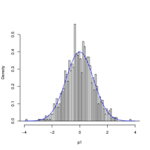
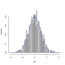
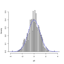
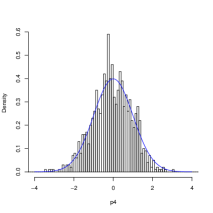
Figure 5: Histogram $p_{i}$ and the density of $\mbox{$\mathrm{N}$}(0,1)$ for $2d=4$

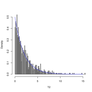
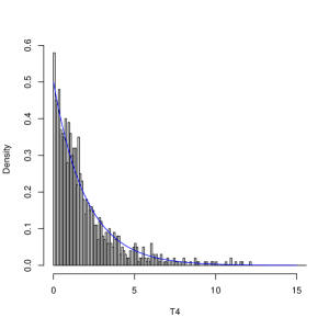
Figure 6: Histogram of $T_{2d-2}$ of (18) and the density of $\chi^{2}(2)$ for $2d=4,6$.

Figure 5 shows for $2d=4$ the histogram of $p_{i}$ and the density of $\mathrm{N(0,1)}$. We see that they agree with each other. Figure 6 shows for $2d=4,6$ the histogram of $T_{2d-2}$ of (18) and the density of the chi-square distribution with $2$ d.f. We again see a good agreement.

6 Bivariate exponential-polynomial distribution on the positive orthant

In this section we develop holonomic gradient descent for bivariate exponential-polynomial distribution on the positive orthant. The differential equations needed for HGD are more difficult to derive than in the univariate case. Also the problem of singularity of the system of differential equations arises in the bivariate case.

Let

$$h(\mbox{\boldmath$\theta$},x,y) =\exp\left(\sum\limits_{0\leq i+j\leq d}\theta_{ij}x^{i}y^{j}\right)$$

$$=\exp(\theta_{10}x+\theta_{01}y+\theta_{20}x^{2}+\theta_{11}xy+\theta_{02}y^{2}+\cdots+\theta_{d0}x^{d}+\cdots+\theta_{0d}y^{d})$$

and consider the density function

$$f(x,y;\bm{\theta})=\frac{{1}}{A(\mbox{\boldmath$\theta$})}h(\mbox{\boldmath$\theta$},x,y),$$

where

$$A(\mbox{\boldmath$\theta$})=\int_{0}^{\infty}\int_{0}^{\infty}h(\mbox{\boldmath$\theta$},x,y)\mbox{$\mathrm{d}$}x\mbox{$\mathrm{d}$}y$$

is the normalizing constant. We call this distribution a bivariate exponential-polynomial distribution of degree $d$. Here the parameter vector $\theta$ belongs to the parameter space

$$\mbox{\boldmath$\Theta$}=\{\mbox{\boldmath$\theta$}\mid A(\mbox{\boldmath$\theta$})<\infty\}.$$ (20)

We consider the structure of $\Theta$ below in Section 6.3. We note that if $\mbox{\boldmath$\theta$}\in\mbox{\boldmath$\Theta$}$, then $h(\mbox{\boldmath$\theta$},x,y)$ satisfies

$$h(\mbox{\boldmath$\theta$},x,y) \rightarrow 0\qquad(x\rightarrow\infty),$$ (21)

$$h(\mbox{\boldmath$\theta$},x,y) \rightarrow 0\qquad(y\rightarrow\infty).$$

Given the sample $\mbox{\boldmath$z$}=\{(x_{i},y_{i})\}_{i=1}^{n}$, $(1/n)$ times the log-likelihood function is written as

$$\bar{l}(\mbox{\boldmath$\theta$},\mbox{\boldmath$z$}) =\sum\limits_{1\leq s+t\leq d}\theta_{st}\overline{x^{s}y^{t}}-\log A(\mbox{\boldmath$\theta$})$$ (22)

$$=\theta_{10}\overline{x}+\theta_{01}\overline{y}+\cdots+\theta_{st}\overline{x^{s}y^{t}}+\cdots+\theta_{d0}\overline{x^{d}}+\cdots+\theta_{0d}\overline{y^{d}}-\log A(\mbox{\boldmath$\theta$}),$$

where $\overline{x^{s}y^{t}}=(1/n)\sum_{i=1}^{n}x_{i}^{s}y_{i}^{t}$. From (22) the gradient vectors is given as

$$\nabla\bar{l}(\mbox{\boldmath$\theta$},\mbox{\boldmath$z$})=\begin{bmatrix}\overline{x}\\ \overline{y}\\ \vdots\\ \overline{x^{s}y^{t}}\\ \vdots\\ \overline{x^{d}}\\ \overline{x^{d-1}y}\\ \vdots\\ \overline{y^{d}}\end{bmatrix}-\frac{1}{A(\mbox{\boldmath$\theta$})}\begin{bmatrix}\partial_{10}A(\mbox{\boldmath$\theta$})\\ \partial_{01}A(\mbox{\boldmath$\theta$})\\ \vdots\\ \partial_{st}A(\mbox{\boldmath$\theta$})\\ \vdots\\ \partial_{d0}A(\mbox{\boldmath$\theta$})\\ \partial_{d-1,1}A(\mbox{\boldmath$\theta$})\\ \vdots\\ \partial_{0d}A(\mbox{\boldmath$\theta$})\end{bmatrix},$$ (23)

where $\partial_{ij}=\partial/\partial\theta_{ij}$. As in the univariate case we would like to avoid numerical integration for $\partial_{ij}A(\mbox{\boldmath$\theta$})$, $0\leq i+j\leq d$, in every step of iteration for obtaining MLE.

6.1 Maximum likelihood estimation for the bivariate case

We first derive differential equations satisfied by $A(\mbox{\boldmath$\theta$})$. Since there are terms like $xy$, we need to obtain different types of differential equations, which were not needed in the univariate case.

Let

$$A_{x}(\mbox{\boldmath$\theta$}) =\int_{0}^{\infty}h(\mbox{\boldmath$\theta$},x,0)\mbox{$\mathrm{d}$}x=\int_{0}^{\infty}\exp(\theta_{10}x+\theta_{20}x^{2}+\cdots+\theta_{d0}x^{d})\mbox{$\mathrm{d}$}x,$$ (24)

$$A_{y}(\mbox{\boldmath$\theta$}) =\int_{0}^{\infty}h(\mbox{\boldmath$\theta$},0,y)\mbox{$\mathrm{d}$}y=\int_{0}^{\infty}\exp(\theta_{01}y+\theta_{02}y^{2}+\cdots+\theta_{0d}y^{d})\mbox{$\mathrm{d}$}y.$$ (25)

The values of (24), (25) and their derivatives with respect to $\theta_{ij}$ can be obtained easily from our results for the univariate case. Hence in the following derivation we treat them as known or already evaluated.

We differentiate $A(\mbox{\boldmath$\theta$})$ by $\theta_{01}$ or $\theta_{10}$. Then

$$\partial_{10}A(\mbox{\boldmath$\theta$})=\int_{0}^{\infty}\int_{0}^{\infty}xh(\mbox{\boldmath$\theta$},x,y)\mbox{$\mathrm{d}$}x\mbox{$\mathrm{d}$}y,\quad\partial_{01}A(\mbox{\boldmath$\theta$})=\int_{0}^{\infty}\int_{0}^{\infty}yh(\mbox{\boldmath$\theta$},x,y)\mbox{$\mathrm{d}$}x\mbox{$\mathrm{d}$}y$$

and we have

$$\partial_{10}^{s}\partial_{01}^{t}A(\mbox{\boldmath$\theta$})=\int_{0}^{\infty}\int_{0}^{\infty}x^{s}y^{t}h(\mbox{\boldmath$\theta$},x,y)\mbox{$\mathrm{d}$}x\mbox{$\mathrm{d}$}y.$$ (26)

On the other hand,

$$\partial_{st}A(\mbox{\boldmath$\theta$})=\int_{0}^{\infty}\int_{0}^{\infty}x^{s}y^{t}h(\mbox{\boldmath$\theta$},x,y)\mbox{$\mathrm{d}$}x\mbox{$\mathrm{d}$}y.$$ (27)

From (26), (27) we have

$$(\partial_{st}-\partial_{10}^{s}\partial_{01}^{t})A(\mbox{\boldmath$\theta$})=0.$$

Furthermore corresponding to Theorem 2.1, we have the following theorem.

Theorem 6.1.

$A(\mbox{\boldmath$\theta$})$ satisfies the following differential equations.

$$\left(\sum\limits_{1\leq i+j\leq d,1\leq i}i\theta_{ij}\partial_{10}^{i-1}\partial_{01}^{j}\right)A(\mbox{\boldmath$\theta$}) =-A_{y}(\mbox{\boldmath$\theta$}),$$ (28)

$$\left(\sum\limits_{1\leq i+j\leq d,1\leq j}j\theta_{ij}\partial_{10}^{i}\partial_{01}^{j-1}\right)A(\mbox{\boldmath$\theta$}) =-A_{x}(\mbox{\boldmath$\theta$}).$$ (29)

Proof.

By symmetry we only show (28). We have

$$\int_{0}^{\infty}\int_{0}^{\infty}\partial_{x}h(\mbox{\boldmath$\theta$},x,y)\mbox{$\mathrm{d}$}x\mbox{$\mathrm{d}$}y =\int_{0}^{\infty}\left\{\int_{0}^{\infty}\partial_{x}h(\mbox{\boldmath$\theta$},x,y)\mbox{$\mathrm{d}$}x\right\}\mbox{$\mathrm{d}$}y$$

$$=\int_{0}^{\infty}\left[h(\mbox{\boldmath$\theta$},x,y)\right]_{x=0}^{x=\infty}\mbox{$\mathrm{d}$}y=-\int_{0}^{\infty}h(\bm{\theta},0,y)\mathrm{d}y\qquad(\text{by }\eqref{eq:proposal_x})$$

$$=-A_{y}(\mbox{\boldmath$\theta$}).$$ (30)

On the other hand,

$$\int_{0}^{\infty}\int_{0}^{\infty}\partial_{x}h(\mbox{\boldmath$\theta$},x,y)\mbox{$\mathrm{d}$}x\mbox{$\mathrm{d}$}y =\int_{0}^{\infty}\int_{0}^{\infty}\partial_{x}\exp\big{(}\sum\limits_{0\leq i+j\leq d}\theta_{ij}x^{i}y^{j}\big{)}\mbox{$\mathrm{d}$}x\mbox{$\mathrm{d}$}y$$

$$=\int_{0}^{\infty}\int_{0}^{\infty}\left(\sum\limits_{1\leq i+j\leq d,1\leq i}i\theta_{ij}x^{i-1}y^{j}\right)\exp(\sum\limits_{0\leq i+j\leq d}\theta_{ij}x^{i}y^{j})\mbox{$\mathrm{d}$}x\mbox{$\mathrm{d}$}y$$

$$=\left(\sum\limits_{1\leq i+j\leq d,1\leq i}i\theta_{ij}\partial_{10}^{i-1}\partial_{01}^{j}\right)\int_{0}^{\infty}\int_{0}^{\infty}h(\mbox{\boldmath$\theta$},x,y)\mbox{$\mathrm{d}$}x\mbox{$\mathrm{d}$}y\qquad(\text{by }\eqref{eq:diff-eq-3-1-2})$$

$$=\left(\sum\limits_{1\leq i+j\leq d,1\leq i}i\theta_{ij}\partial_{10}^{i-1}\partial_{01}^{j}\right)A(\mbox{\boldmath$\theta$}).$$ (31)

(28) follows from (30) and (31). ∎

In the univariate case, the important fact was that higher-order derivatives of $A_{d}(\mbox{\boldmath$\theta$})$ are written as rational function combinations of lower-order derivatives of $A_{d}(\mbox{\boldmath$\theta$})$. In (28), (29), the highest order of derivatives in $A_{d}(\mbox{\boldmath$\theta$})$ is $d-1$ and there are $d$ derivatives of order $d-1$:

$$\partial_{10}^{d-1},\partial_{10}^{d-2}\partial_{01},\cdots,\partial_{10}\partial_{01}^{d-2},\partial_{01}^{d-1}.$$

If we want to evaluate these $d$ derivatives of order $d-1$ by solving a system of equations, then we do not have enough equations for $d\geq 3$, because there are only two equations in Theorem 6.1. We need to have more differential equations.

To obtain more equations, we operate the following set

$$O_{q}=\{\partial_{10}^{q},\partial_{10}^{q-1}\partial_{01},\partial_{10}^{q-2}\partial_{01}^{2},\cdots,\partial_{01}^{q}\}$$

of $q+1$ differential operators of the same order $q$ to (28) and (29). In order to determine $q$, we count the number of differential equations obtained after operating $O_{q}$.

The highest order of derivatives after operating $O_{q}$ to (28), (29) is $q+d-1$ and there are the following $q+d$ derivatives

$$\partial_{10}^{q+d-1},\partial_{10}^{q+d-2}\partial_{01},\cdots,\partial_{10}\partial_{01}^{q+d-2},\partial_{01}^{q+d-1}.$$

On the other hand there are $2(q+1)$ differential equations after operating $O_{q}$ to (28), (29). Hence we have the right number of equations if we take $q+d=2(q+1)$ or

$$q=d-2.$$

In view of

$$\partial_{10}A_{y}(\mbox{\boldmath$\theta$})=0,\qquad\partial_{01}A_{x}(\mbox{\boldmath$\theta$})=0,$$

when we operate

$$O_{d-2}=\{\partial_{10}^{d-2},\partial_{10}^{d-3}\partial_{01},\partial_{10}^{d-4}\partial_{01}^{2},\cdots,\partial_{01}^{d-2}\}$$

to (28), (29), we have the following system of differential equations.

$$\begin{bmatrix}\partial_{10}^{d-2}&0\\ \partial_{10}^{d-3}\partial_{01}&\vdots\\ \vdots&\vdots\\ \partial_{10}\partial_{01}^{d-3}&\vdots\\ \partial_{01}^{d-2}&0\\ 0&\partial_{10}^{d-2}\\ \vdots&\partial_{10}^{d-3}\partial_{0\,1}\\ \vdots&\vdots\\ \vdots&\partial_{10}\partial_{01}^{d-3}\\ 0&\partial_{01}^{d-2}\end{bmatrix}\begin{bmatrix}\left(\sum\limits_{1\leq i+j\leq d,1\leq i}i\theta_{ij}\partial_{10}^{i-1}\partial_{01}^{j}\right)A(\mbox{\boldmath$\theta$})\\ \left(\sum\limits_{1\leq i+j\leq d,1\leq j}j\theta_{ij}\partial_{10}^{i}\partial_{01}^{j-1}\right)A(\mbox{\boldmath$\theta$})\\ \end{bmatrix} =\begin{bmatrix}\partial_{10}^{d-2}&0\\ \partial_{10}^{d-3}\partial_{01}&\vdots\\ \vdots&\vdots\\ \partial_{10}\partial_{01}^{d-3}&\vdots\\ \partial_{01}^{d-2}&0\\ 0&\partial_{10}^{d-2}\\ \vdots&\partial_{10}^{d-3}\partial_{01}\\ \vdots&\vdots\\ \vdots&\partial_{10}\partial_{01}^{d-3}\\ 0&\partial_{01}^{d-2}\end{bmatrix}\begin{bmatrix}-A_{y}(\mbox{\boldmath$\theta$})\\ -A_{x}(\mbox{\boldmath$\theta$})\end{bmatrix}=-\begin{bmatrix}0\\ \vdots\\ 0\\ \partial_{01}^{d-2}A_{y}(\mbox{\boldmath$\theta$})\\ \partial_{10}^{d-2}A_{x}(\mbox{\boldmath$\theta$})\\ 0\\ \vdots\\ 0\end{bmatrix}$$ (32)

We transform (32) to a system of differential equations to solve for the derivatives of the highest order

$$\partial_{10}^{2d-3},\partial_{10}^{2d-4}\partial_{01},\cdots,\partial_{10}\partial_{01}^{2d-4},\partial_{01}^{2d-3}.$$

For any pair of non-negative integers $(s,t)$ satisfying $s+t=d-2$ let

$$\begin{split}\phi(s,t)&=s\partial_{10}^{s-1}\partial_{01}^{t}+\theta_{10}\partial_{10}^{s}\partial_{01}^{t}+\sum\limits_{2\leq i+j\leq d-1,1\leq i}i\theta_{ij}\partial_{10}^{s+i-1}\partial_{01}^{j+t},\\ \psi(s,t)&=t\partial_{10}^{s}\partial_{01}^{t-1}+\theta_{01}\partial_{10}^{s}\partial_{01}^{t}+\sum\limits_{2\leq i+j\leq d-1,1\leq j}j\theta_{ij}\partial_{10}^{s+i}\partial_{01}^{t+j-1}.\end{split}$$ (33)

Then (32) is transformed to

$$\begin{cases}\sum\limits_{i+j=d,1\leq i}i\theta_{ij}\partial_{10}^{s+i-1}\partial_{01}^{t+j}A(\mbox{\boldmath$\theta$})=-\partial_{10}^{s}\partial_{01}^{t}A_{y}(\mbox{\boldmath$\theta$})-\phi(s,t)A(\mbox{\boldmath$\theta$}),&\\ \sum\limits_{i+j=d,1\leq j}j\theta_{ij}\partial_{10}^{s+i}\partial_{01}^{t+j-1}A(\mbox{\boldmath$\theta$})=-\partial_{10}^{s}\partial_{01}^{t}A_{x}(\mbox{\boldmath$\theta$})-\psi(s,t)A(\mbox{\boldmath$\theta$}).&\end{cases}\$$ (34)

In matrix form (34) is expressed as

$$P(\mbox{\boldmath$\theta$})\begin{bmatrix}\partial_{10}^{2d-3}A(\mbox{\boldmath$\theta$})\\ \partial_{10}^{2d-4}\partial_{01}A(\mbox{\boldmath$\theta$})\\ \vdots\\ \partial_{10}\partial_{01}^{2d-4}A(\mbox{\boldmath$\theta$})\\ \partial_{01}^{2d-3}A(\mbox{\boldmath$\theta$})\end{bmatrix}=Q(\mbox{\boldmath$\theta$}),$$

where

$$\begin{matrix}P(\mbox{\boldmath$\theta$})=\begin{bmatrix}d\theta_{d0}&\cdots&\cdots&2\theta_{2,d-2}&\theta_{1,d-1}\\ &d\theta_{d0}&\cdots&\cdots&2\theta_{2,d-2}&\theta_{1,d-1}\\ &&&\cdots&\cdots\\ &&&d\theta_{d0}&\cdots&\cdots&2\theta_{2,d-2}&\theta_{1,d-1}\\ \theta_{d-1,1}&2\theta_{d-2,2}&\cdots&\cdots&d\theta_{0d}\\ &\theta_{d-1,1}&2\theta_{d-2,2}&\cdots&\cdots&d\theta_{0d}\\ &&&\cdots&\cdots\\ &&&\theta_{d-1,1}&2\theta_{d-2,2}&\cdots&\cdots&d\theta_{0d}\\ \end{bmatrix}\begin{aligned} &\left.\begin{matrix}\\ \\ \\ \\ \end{matrix}\right\}\text{$(d-1)$ rows}\\ &\left.\begin{matrix}\\ \\ \\ \\ \end{matrix}\right\}\text{$(d-1)$ rows}\\ \end{aligned}\end{matrix},$$ (35)

$$Q(\mbox{\boldmath$\theta$})=-\begin{bmatrix}\phi(d-2,0)A(\mbox{\boldmath$\theta$})\\ \phi(d-3,1)A(\mbox{\boldmath$\theta$})\\ \vdots\\ \phi(1,d-3)A(\mbox{\boldmath$\theta$})\\ \partial_{01}^{d-2}A_{y}(\mbox{\boldmath$\theta$})+\phi(0,d-2)A(\mbox{\boldmath$\theta$})\\ \partial_{10}^{d-2}A_{x}(\mbox{\boldmath$\theta$})+\psi(d-2,0)A(\mbox{\boldmath$\theta$})\\ \psi(d-3,1)A(\mbox{\boldmath$\theta$})\\ \vdots\\ \psi(1,d-3)A(\mbox{\boldmath$\theta$})\\ \psi(0,d-2)A(\mbox{\boldmath$\theta$})\\ \end{bmatrix}.$$ (36)

In $P(\mbox{\boldmath$\theta$})$ empty elements in the matrix are zeros. We give further consideration of $P(\mbox{\boldmath$\theta$})$ in the next section.

If $\det P(\mbox{\boldmath$\theta$})\neq 0$,

$$\begin{bmatrix}\partial_{10}^{2d-3}A(\mbox{\boldmath$\theta$})\\ \partial_{10}^{2d-4}\partial_{01}A(\mbox{\boldmath$\theta$})\\ \vdots\\ \partial_{10}\partial_{01}^{2d-4}A(\mbox{\boldmath$\theta$})\\ \partial_{01}^{2d-3}A(\mbox{\boldmath$\theta$})\end{bmatrix}=P^{-1}(\mbox{\boldmath$\theta$})Q(\mbox{\boldmath$\theta$}).$$ (37)

Hence from (33), (36), (37) we see that $\partial_{10}^{2d-3}A(\mbox{\boldmath$\theta$}),\partial_{10}^{2d-4}\partial_{01}A(\mbox{\boldmath$\theta$}),\cdots,\partial_{10}\partial_{01}^{2d-4}A(\mbox{\boldmath$\theta$}),\partial_{01}^{2d-3}A(\mbox{\boldmath$\theta$}),$ are written as rational function combinations of elements of the vector

$$F(\mbox{\boldmath$\theta$})=[A(\mbox{\boldmath$\theta$}),\partial_{10}A(\mbox{\boldmath$\theta$}),\partial_{01}A(\mbox{\boldmath$\theta$}),\cdots,\partial_{10}^{2d-4}A(\mbox{\boldmath$\theta$}),\partial_{10}^{2d-5}\partial_{01}A(\mbox{\boldmath$\theta$}),\cdots,\partial_{10}\partial_{01}^{2d-5}A(\mbox{\boldmath$\theta$}),\partial_{01}^{2d-4}A(\mbox{\boldmath$\theta$})]^{\mathsf{T}}.$$ (38)

If we can evaluate $F(\mbox{\boldmath$\theta$})$ at any $\theta$, then by (23) we can obtain the maximum likelihood estimate of the bivariate exponential-polynomial distribution. As in the univariate case, if the initial values of $F(\mbox{\boldmath$\theta$}_{0})$ can be evaluated at $\mbox{\boldmath$\theta$}_{0}$, then the value of $F(\mbox{\boldmath$\theta$})$ at any other point $\theta$ can be obtained by solving the differential equation.

In the univariate case, the origin $\theta_{d}=0$ was the only singular point of the differential equation (6). In the bivariate case the set $\{\bm{\theta}|\det P(\bm{\theta})=0\}$ is the set of singularities of (32). This singularity causes difficulty for HGD and in the next section we investigate $\det P(\bm{\theta})$.

Remark 6.2.

As in Remark 2.2, $A(\bm{\theta})$ satisfies an incomplete $A$-hypergeometric system.

6.2 Evaluation of the determinant of the Pfaffian system

We prove that $\det P(\mbox{\boldmath$\theta$})$ in (35) is given by the discriminant of a polynomial equation. We use the basic results on determinantal expression for resultants and discriminants (cf. Chapter 12 of [4], Section 3.3 of [1]). Let two polynomials $f(x)$, $g(x)$ be denoted as

$$f(x) =a_{m}x^{m}+a_{m-1}x^{m-1}+\cdots+a_{0}=a_{m}\prod_{i=1}^{m}(x-\alpha_{i}),$$ (39)

$$g(x) =b_{n}x^{n}+b_{m-1}x^{m-1}+\cdots+b_{0}=b_{n}\prod_{i=1}^{n}(x-\beta_{i}).$$

The resultant $R(f,g)$ is defined as

$$R(f,g)=a_{m}^{n}b_{n}^{m}\prod_{i=1}^{m}\prod_{j=1}^{n}(\alpha_{i}-\beta_{j}).$$

Then the determinantal expression of $R(f,g)$ is given as follows ((1.12) of Chapter 12 of [4], Lemma 3.3.4 of [1]).

$$\begin{matrix}R(f,g)=\det\begin{bmatrix}a_{m}&a_{m-1}&\cdots&\cdots&\cdots&a_{0}\\ &a_{n}&a_{m-1}&\cdots&\cdots&\cdots&a_{0}\\ &&&&\cdots&\cdots&\cdots\\ &&&a_{m}&a_{m-1}&\cdots&\cdots&\cdots&a_{0}\\ b_{n}&b_{n-1}&\cdots&b_{0}\\ &b_{n}&b_{n-1}&\cdots&b_{0}\\ &&&&\cdots\\ &&&&&\cdots\\ &&&&&&\cdots\\ &&&&&b_{n}&b_{n-1}&\cdots&b_{0}\end{bmatrix}\begin{aligned} &\left.\begin{matrix}\\ \\ \\ \\ \end{matrix}\right\}\text{$n$ rows}\\ &\left.\begin{matrix}\\ \\ \\ \\ \\ \\ \end{matrix}\right\}\text{$m$ rows}\\ \end{aligned}\end{matrix}$$

We also consider the discriminant. For $f(x)$ in (39) the discriminant for the equation $f(x)=0$ is given by

$$D=(-1)^{m(m-1)/2}a_{m}^{2(m-1)}\prod_{1\leq i<j\leq m}(\alpha_{i}-\alpha_{j})^{2}.$$

Let

$$p(x;\mbox{\boldmath$\theta$})=\theta_{d0}x^{d}+\theta_{d-1,1}x^{d-1}+\theta_{d-2,2}x^{d-2}+\cdots+\theta_{1,d-1}x+\theta_{0d}.$$ (40)

This polynomial will also appear in the next section in the investigation of the parameter space $\Theta$ in (20). The discriminant $D(\mbox{\boldmath$\theta$})$ of the polynomial equation $p(x,\mbox{\boldmath$\theta$})=0$ is given as ((1.29) of Chapter 12 of [4], Definition 3.3.3 of [1])

$$D(\mbox{\boldmath$\theta$})=\frac{1}{\theta_{d0}}R(p,p^{\prime}),$$ (41)

where

$$\begin{matrix}R(p,p^{\prime})=\det\begin{bmatrix}\theta_{d0}&\theta_{d-1,1}&\cdots&\cdots&\cdots&\theta_{0d}\\ &\theta_{d0}&\theta_{d-1,1}&\cdots&\cdots&\cdots&\theta_{0d}\\ &&&&\cdots&\cdots&\cdots\\ &&&\theta_{d0}&\theta_{d-1,1}&\cdots&\cdots&\cdots&\theta_{0d}\\ d\theta_{d0}&\cdots&\cdots&2\theta_{2,d-2}&\theta_{1,d-1}\\ &d\theta_{d0}&\cdots&\cdots&2\theta_{2,d-2}&\theta_{1,d-1}\\ &&&\cdots&\cdots\\ &&&&\cdots&\cdots\\ &&&&d\theta_{d0}&\cdots&\cdots&2\theta_{2,d-2}&\theta_{1,d-1}\end{bmatrix}\begin{aligned} &\left.\begin{matrix}\\ \\ \\ \\ \end{matrix}\right\}\text{$(d-1)$ rows}\\ &\left.\begin{matrix}\\ \\ \\ \\ \\ \end{matrix}\right\}\text{$d$ rows}\\ \end{aligned}\end{matrix}.$$

Using (41) we give the following theorem on the relation of $\det P(\mbox{\boldmath$\theta$})$ in (35) and the discriminant $D(\mbox{\boldmath$\theta$})$ of polynomial equation $p(x;\bm{\theta})=0$ in (40).

Theorem 6.3.

$$\det P(\mbox{\boldmath$\theta$})=d^{d-2}D(\mbox{\boldmath$\theta$}).$$ (42)

Proof.

Define a $(2d-1)\times(2d-1)$ matrix $S$ as

$$S=\begin{bmatrix}\theta_{d0}&0&-\theta_{d-2,2}&-2\theta_{d-3,3}&\cdots&-(d-1)\theta_{0d}&0&\cdots&0\\ {\bm{0}}&&&&P(\mbox{\boldmath$\theta$})\end{bmatrix},$$

where ${\bm{0}}$ is a column vector of zeros of size $2d-2$. Expanding the determinant with respect to the fist column we have

$$\det S=\theta_{d0}\det P(\mbox{\boldmath$\theta$}).$$ (43)

On the other hand we add the $i$-row to the $(i+d)$-th rows $(1\leq i\leq d-1)$ and then add the $(d+1)$-st row multiplied by $d-1$ to the first row. Then we obtain

$$\det S=d^{d-2}\det\begin{bmatrix}d\theta_{d0}&\cdots&\cdots&2\theta_{2,d-2}&\theta_{1,d-1}\\ &d\theta_{d0}&\cdots&\cdots&2\theta_{2,d-2}&\theta_{1,d-1}\\ &&&\cdots&\cdots\\ &&&&\cdots&\cdots\\ &&&&d\theta_{d0}&\cdots&\cdots&2\theta_{2,d-2}&\theta_{1,d-1}\\ \theta_{d0}&\theta_{d-1,1}&\cdots&\cdots&\cdots&\theta_{0d}\\ &\theta_{d0}&\theta_{d-1,1}&\cdots&\cdots&\cdots&\theta_{0d}\\ &&&&\cdots&\cdots&\cdots\\ &&&\theta_{d0}&\theta_{d-1,1}&\cdots&\cdots&\cdots&\theta_{0d}\end{bmatrix}.$$

By interchanging rows

$$\det S =d^{d-2}(-1)^{d(d-1)}R(p,p^{\prime})$$

$$=\theta_{d0}d^{d-2}\det D(\mbox{\boldmath$\theta$}).\qquad(\text{by}\ \eqref{eq:det-matrix})$$ (44)

From (43), (6.2) we have

$$\det P(\mbox{\boldmath$\theta$})=d^{d-2}D(\mbox{\boldmath$\theta$}).$$

∎

One of the reviewers asked the question of invariance of the singularities under transformations of parameters. The class of holonomic functions are closed under rational transformations of arguments. Hence if the parameters $\theta_{ij}$ are transformed by a rational transformation, the singularity of the Pfaffian system remains to be the singularity, although the transformation itself may add its own (removable) singularity.

6.3 Structure of the parameter space for the bivariate case

In this section we investigate the parameter space $\Theta$. By the transformation

$$x=r\cos\omega,\quad y=r\sin\omega,$$

define

$$H(\bm{\theta},\omega)=\int_{0}^{\infty}\tilde{h}(\mbox{\boldmath$\theta$},r,\omega)\mbox{$\mathrm{d}$}r,\quad\tilde{h}(\mbox{\boldmath$\theta$},r,\omega)=rh(\mbox{\boldmath$\theta$},r\cos\omega,r\sin\omega).$$

Since $\tilde{h}$ is non-negative, by Fubini’s theorem $A(\mbox{\boldmath$\theta$})$ is written as

$$A(\mbox{\boldmath$\theta$})=\int_{0}^{\pi/2}H(\bm{\theta},\omega)\mbox{$\mathrm{d}$}\omega.$$

Note that $\log h(\bm{\theta},r\cos\omega,r\sin\omega)$ is a polynomial in $r$ for each $\omega\in[0,\pi/2]$ . Since the limit of $\log h(\bm{\theta},r\cos\omega,r\sin\omega)$ as $r\rightarrow\infty$ is $+\infty$ of $-\infty$, depending on the sign of the leading coefficient (i.e. the highest non-zero coefficient for a power) of $r$, we have

$$H(\bm{\theta},\omega)<\infty\ \ \Leftrightarrow\ \ h(\mbox{\boldmath$\theta$},r\cos\omega,r\sin\omega)\rightarrow 0\quad(r\rightarrow\infty).$$

Write $a=1/\tan\omega$. The coefficient of the highest degree term in $y$ of $\log h(\bm{\theta},ay,y)$ is $p(a;\mbox{\boldmath$\theta$})$, where $p(x;\mbox{\boldmath$\theta$})$ is given in (40). If $p(a;\mbox{\boldmath$\theta$})<0$ for all $a\geq 0$, then $\theta_{0d}$ and the leading coefficient of $p(a;\mbox{\boldmath$\theta$})$ are negative. By interchanging the roles of $x$ and $y$ we also assume that the leading coefficient of $p(a;\mbox{\boldmath$\theta$})$ is $\theta_{d0}$. Note that $p(a;\mbox{\boldmath$\theta$})<0$ for all $a\geq 0$ implies $\sup_{a\geq 0}p(a;\mbox{\boldmath$\theta$})<0$. Define

$$\mbox{\boldmath$\Theta$}^{\prime}=\{\mbox{\boldmath$\theta$}\mid p(a;\mbox{\boldmath$\theta$})<0,\forall a\geq 0,\ \theta_{0d}<0,\theta_{d0}<0\}.$$ (45)

Then we have $\mbox{\boldmath$\Theta$}^{\prime}\subset\mbox{\boldmath$\Theta$}$. Note that for $\bm{\theta}\in\mbox{\boldmath$\Theta$}\setminus\mbox{\boldmath$\Theta$}^{\prime}$ there exists $a>0$ such that $p(a;\bm{\theta})=0$, i.e., the term of order $d$ in $y$ vanishes on the ray $\{(ay,y),y\geq 0\}$. In this sense $\bm{\theta}\in\mbox{\boldmath$\Theta$}\setminus\mbox{\boldmath$\Theta$}^{\prime}$ may be considered as a model of order $d-1$. We call $\mbox{\boldmath$\Theta$}^{\prime}$ in (45) the parameter space of a proper order-$d$ model.

Remark 6.4.

One of the reviewers gave very interesting examples concerning the continuity of $H(\bm{\theta},\omega)$ and the relation between the convergence (finiteness) of $A(\bm{\theta})$ and the convergence of $H(\bm{\theta},\omega)$ for each $\omega\in[0,\pi/2]$.

• Let $h(\bm{\theta},x,y)=\exp(x^{2}-y^{2}-x)$. Then $H(\bm{\theta},\omega)=\infty$ for $\omega<\pi/4$, but $H(\bm{\theta},\pi/4)<\infty$.

• Let $h(\bm{\theta},x,y)=\exp(-(y-x^{2})^{2})$. Then $H(\bm{\theta},\omega)<\infty$ for each $\omega\in[0,\pi/2]$ but $A(\bm{\theta})=\infty$.

• Let $h(\bm{\theta},x,y)=\exp(-(x-y)^{2}(x^{2}+y^{2})^{2})$. Then $H(\bm{\theta},\pi/4)=\infty$ but $A(\bm{\theta})<\infty.$

These examples illustrate the difficulty in characterizing the boundary of $\Theta$.

The above consideration gives insight into the structure of $\Theta$, but it is still difficult to decide whether $\mbox{\boldmath$\theta$}\in\mbox{\boldmath$\Theta$}^{\prime}$ for a given $\theta$. We propose the following easier method for determination. Now clearly we have

$$p(x;\mbox{\boldmath$\theta$})<0\quad(\forall x\geq 0)\ \Leftrightarrow\ p(x;\mbox{\boldmath$\theta$})\text{ does not have a positive root.}$$

Following the argument in [2], we now move $\theta$ from an initial point in $\mbox{\boldmath$\Theta$}^{\prime}$, keeping $\theta_{d0}<0,\theta_{0d}<0$, and consider when $p(x;\mbox{\boldmath$\theta$})$ is no longer negative for some $x>0$, i.e., when $p(x;\mbox{\boldmath$\theta$})=0$ has a positive root. There are two cases.

1. A real root moves from the negative real line to the positive real line.

2. A complex root moves to the positive real line.

The first case corresponds to $\theta_{0d}>0$, but this does not happen by our assumption. Complex roots for a polynomial with real coefficients appear in conjugate pairs and in the second case we have a multiple root on the positive real line. Hence under the assumption $\theta_{d0}<0,\theta_{0d}<0$, a positive root appears if and only if the discriminant $D(\mbox{\boldmath$\theta$})$ of $p(x;\mbox{\boldmath$\theta$})=0$ becomes $0$ and the root becomes positive. Note that $D(\bm{\theta})=0$ may also happen because of negative or complex multiple roots.

Based on this observation consider the complement of the hypersurface $\{\bm{\theta}\mid D(\bm{\theta})=0\}$ in $\{\mbox{\boldmath$\theta$}\mid\theta_{d0}<0,\theta_{0d}<0\}$:

$$\mbox{\boldmath$\Theta$}^{\prime\prime}=\{\mbox{\boldmath$\theta$}\mid\theta_{d0}<0,\theta_{0d}<0\}\setminus\{\bm{\theta}\mid D(\mbox{\boldmath$\theta$})=0\}$$

$\mbox{\boldmath$\Theta$}^{\prime\prime}$ consists of disjoint open connected components (“chambers”), which we denote by $\mbox{\boldmath$\Theta$}^{\prime\prime}_{i},i\in I$. Then $\mbox{\boldmath$\Theta$}^{\prime\prime}$ is partitioned as

$$\mbox{\boldmath$\Theta$}^{\prime\prime}=\bigcup_{i\in I}\mbox{\boldmath$\Theta$}^{\prime\prime}_{i}.$$

Note that the number of positive roots of $p(x;\bm{\theta})$ is constant in each chamber $\mbox{\boldmath$\Theta$}_{i}^{\prime\prime}$. Hence if $\mbox{\boldmath$\Theta$}^{\prime\prime}_{i}\cap\mbox{\boldmath$\Theta$}^{\prime}\neq\emptyset$, then $\mbox{\boldmath$\Theta$}^{\prime\prime}_{i}\subset\mbox{\boldmath$\Theta$}^{\prime}$, namely each $\mbox{\boldmath$\Theta$}^{\prime\prime}_{i}$ is either a subset of $\mbox{\boldmath$\Theta$}^{\prime}$ or disjoint from $\mbox{\boldmath$\Theta$}^{\prime}$. Define

$$I^{*}=\{i\in I\mid\mbox{\boldmath$\Theta$}^{\prime\prime}_{i}\cap\mbox{\boldmath$\Theta$}^{\prime}\neq\emptyset\}=\{i\in I\mid\mbox{\boldmath$\Theta$}^{\prime\prime}_{i}\subset\mbox{\boldmath$\Theta$}^{\prime}\}.$$

Since the hypersurface $\{\bm{\theta}\mid D(\bm{\theta})=0\}$ has measure zero, we have the following theorem concerning $\mbox{\boldmath$\Theta$}^{\prime}$ in (45).

Theorem 6.5.

Except for a set of measure zero

$$\mbox{\boldmath$\Theta$}^{\prime}=\bigcup_{i\in I^{*}}\mbox{\boldmath$\Theta$}^{\prime\prime}_{i}.$$ (46)

Although it is difficult to completely characterize the boundaries of $\mbox{\boldmath$\Theta$}^{\prime\prime}_{i}$’s for general $d$, if the boundary between ${\mbox{\boldmath$\Theta$}_{i}^{\prime\prime}},i\in I^{*},$ and ${\mbox{\boldmath$\Theta$}_{j}^{\prime\prime}},j\in I^{*},$ corresponds to negative or complex multiple roots, then the boundary also belongs to $\mbox{\boldmath$\Theta$}^{\prime}$.

We illustrate the partition (46) for the case of $d=3$. For any $c_{1},c_{2}>0$, we have $p(x;\bm{\theta})<0,\forall x>0$ if and only if $c_{1}p(c_{2}x;\bm{\theta})<0,\forall x>0$. This implies that we can assume $\theta_{03}=\theta_{30}=-1$ without loss of generality in considering the partition (46). In this case the discriminant is written as

$$D(\bm{\theta})=\theta_{12}^{2}\theta_{21}^{2}+4\theta_{12}^{3}+4\theta_{21}^{3}+18\theta_{12}\theta_{21}-27.$$

On the $(\theta_{12},\theta_{21})$-plane, $D(\bm{\theta})=0$ consists of two curves as illustrated in Figure 7. In Figure 7, chamber $A$ corresponds to two positive roots and one negative root, chamber $B$ corresponds to two complex roots and one negative root, and chamber $C$ corresponds to three negative roots. Hence the partition in (46) is $B\cup C$. The boundary between $B$ and $C$ also belongs to $\mbox{\boldmath$\Theta$}^{\prime}$.

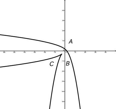
Figure 7: Partition of Theorem 6.5 for $d=3$

For maximum likelihood estimation we need to take an initial point in each chamber $\mbox{\boldmath$\Theta$}^{\prime\prime}_{i}$, $i\in I^{*}$, of Theorem 6.5 and perform the numerical integration only for those initial points. Note that any two points in the same chamber can be connected by a path on which $\det P(\mbox{\boldmath$\theta$})\neq 0$ and the integration of (37) does not depend on the choice of a path. It is difficult to give a simple initial point $\mbox{\boldmath$\Theta$}_{i}^{\prime\prime}$ for all $i\in I^{*}$. For some $i\in I^{*}$, the following simple initial point $\mbox{\boldmath$\theta$}_{0}$ is available. For $c_{1}>0,c_{2}>0$ define $\mbox{\boldmath$\theta$}_{0}$ by

$$\theta_{d0}=-c_{1},\ \theta_{0d}=-c_{2},\quad\theta_{ij}=0\ \ \text{for $(i,j)\neq(0,d),(d,0)$}.$$

Then

$$p(x;\mbox{\boldmath$\theta$}_{0})=-c_{1}x^{d}-c_{2}=0,\quad p^{\prime}(x;\mbox{\boldmath$\theta$}_{0})=-dc_{1}x^{d-1}=0$$

do not have a common root and $R(p,p^{\prime})\neq 0$. Hence $D(\mbox{\boldmath$\theta$}_{0})\neq 0$ and $\det P(\mbox{\boldmath$\theta$})\neq 0$ by (42). Furthermore clearly $p(x;\mbox{\boldmath$\theta$}_{0})$ is negative for $x>0$. Hence $\mbox{\boldmath$\theta$}_{0}\in\mbox{\boldmath$\Theta$}_{i}^{\prime\prime}$, $i\in I^{*}$. For this $\mbox{\boldmath$\theta$}_{0}$ the normalizing constant and its derivatives are easily evaluated as

$$\partial_{ij}A(\mbox{\boldmath$\theta$}_{0}) =\int_{0}^{\infty}\int_{0}^{\infty}x^{i}y^{j}\exp(-c_{1}x^{d}-c_{2}y^{d})\mbox{$\mathrm{d}$}x\mbox{$\mathrm{d}$}y$$

$$=\int_{0}^{\infty}x^{i}\exp(-c_{1}x^{d})\mbox{$\mathrm{d}$}x\int_{0}^{\infty}y^{j}\exp(-c_{2}y^{d})\mbox{$\mathrm{d}$}y$$

$$=\frac{1}{d}c_{1}^{-(i+1)/d}\Gamma\left(\frac{i+1}{d}\right)\frac{1}{d}c_{2}^{-(j+1)/d}\Gamma\left(\frac{j+1}{d}\right).$$

Although we do not show numerical results for the bivariate case, for $d=2$ the computation of the normalizing constant and MLE is fast and the asymptotic distribution of MLE has been checked. For $d=3$, the computation of the normalizing constant is fast, but the computation of MLE is somewhat heavy at current implementation in MATLAB. This seems to be due to high dimensionality (9 parameters) of the model for $d=3$.

7 Some discussions

In this paper we discussed the maximum likelihood estimation of the exponential-polynomial distribution. Here we discuss some possible extensions of the distribution and topics for further research.

In the exponential-polynomial distribution we have a polynomial as the exponent of the exponential function. We can add another polynomial to the exponential-polynomial distribution, if this polynomial is non-negative over the sample space. Recall that the problem concerning non-negative polynomials was also essential for understanding the structure of the parameter space for the bivariate exponential-polynomial distribution in Section 6.3. Let

$$p(x;\bm{\eta})=\eta_{0}+\eta_{1}x+\dots+\eta_{h}x^{h}$$

be a polynomial in $x$. Consider the following density on the positive real line:

$$f(x;\bm{\eta},\bm{\theta}) =\frac{1}{\tilde{A}(\bm{\eta},\bm{\theta})}p(x;\bm{\eta})\exp(\theta_{1}x+\dots+\theta_{d}x^{d}),$$

$$\tilde{A}(\bm{\eta},\bm{\theta}) =\int_{0}^{\infty}p(x;\bm{\eta})\exp(\theta_{1}x+\dots+\theta_{d}x^{d})\mbox{$\mathrm{d}$}x.$$

The normalizing constant $\tilde{A}(\bm{\eta},\bm{\theta})$ can be evaluated as

$$\tilde{A}(\bm{\eta},\bm{\theta})=\sum_{i=0}^{h}\eta_{i}\int_{0}^{\infty}x^{i}\exp(\theta_{1}x+\dots+\theta_{d}x^{d})\\ =\sum_{i=0}^{h}\eta_{i}\partial_{1}^{i}A_{d}(\bm{\theta}),$$

where $A_{d}(\bm{\theta})$ is given in (2). Hence from the view point of holonomic gradient descent this generalization can be easily handled. However, in the estimation of this density we need to guarantee that $p(x;\hat{\bm{\eta}})$ is a non-negative polynomial for $x\geq 0$. This problem was considered in Fushiki et al. ([3]). They showed that the maximum likelihood estimation under the restriction of non-negativity of $p(x;\hat{\bm{\eta}})$ can be performed with the technique of semidefinite programming. We can also use the parameterization of non-negative polynomials given in Proposition 3.3 of [9]. See also Section 9, Chapter V of [8].

For the univariate case we derived score tests for determining the order $d$ of the model. The difficulty in model selection is the fact that the model of order $d-1$ is on the boundary of the model of order $d$. In this paper we did not discuss the problem of model selection for the bivariate case, because the boundary is much more difficult compared to the univariate case, as discussed in Section 6.3. Also in the bivariate case, as the model of order $d$ we included all monomials $x^{d},x^{d-1}y,\dots,y^{d}$ of order $d$. However we may omit some monomials among these $d+1$ monomials. The structure of the boundary of the model seems to depend on the choice of monomials of order $d$. Model selection procedures for the bivariate case is left to a future study.

It is of interest to generalize our results for bivariate case to higher dimensions. As remarked in Remarks 2.2 and 6.2 we can use general theory of $A$-hypergeometric systems to obtain results for the exponential-polynomial distribution in general dimension. In the bivariate case the singularity of the Pfaffian system is described in terms of the discriminant $D(\mbox{\boldmath$\theta$})$ in Theorem 6.3. It is of interest to generalize this result to higher dimensions.

Acknowledgment   The authors are very grateful to Satoshi Kuriki, Nobuki Takayama, Tamio Koyama and two reviewers for very useful suggestions.

References

- [1] H. Cohen. A Course in Computational Algebraic Number Theory, volume 138 of Graduate Texts in Mathematics. Springer-Verlag, Berlin, 1993.
- [2] N. Fukuma and T. Mori. On positivity of linear combinations of polynomials. IEEJ Transactions on Electronics, Information and Systems, 113(10):798–803, 1993. (In Japanese).
- [3] T. Fushiki, S. Horiuchi, and T. Tsuchiya. A maximum likelihood approach to density estimation with semidefinite programming. Neural Comput., 18(11):2777–2812, 2006.
- [4] I. M. Gelfand, M. M. Kapranov, and A. V. Zelevinsky. Discriminants, Resultants and Multidimensional Determinants. Modern Birkhäuser Classics. Birkhäuser Boston Inc., Boston, MA, 2008. Reprint of the 1994 edition.
- [5] H. Hashiguchi, Y. Numata, N. Takayama, and A. Takemura. Holonomic gradient method for the distribution function of the largest root of a Wishart matrix. Journal of Multivariate Analysis, 117:296–312, 2013.
- [6] T. Hibi, editor. Grobner Bases: Statistics and Software Systems. Springer, Tokyo, Japan, 2013.
- [7] N. L. Johnson, S. Kotz, and N. Balakrishnan. Continuous Univariate Distributions. Vol. 1. Wiley Series in Probability and Mathematical Statistics: Applied Probability and Statistics. John Wiley & Sons Inc., New York, second edition, 1994. A Wiley-Interscience Publication.
- [8] S. Karlin and W. J. Studden. Tchebycheff Systems: With Applications in Analysis and Statistics. Pure and Applied Mathematics, Vol. XV. John Wiley & Sons Inc., 1966.
- [9] N. Kato and S. Kuriki. Likelihood ratio tests for positivity in polynomial regressions. J. Multivariate Anal., 115:334–346, 2013.
- [10] E. L. Lehmann. Elements of Large-Sample Theory. Springer Texts in Statistics. Springer-Verlag, New York, 1999.
- [11] H. Nakayama, K. Nishiyama, M. Noro, K. Ohara, T. Sei, N. Takayama, and A. Takemura. Holonomic gradient descent and its application to the Fisher-Bingham integral. Adv. in Appl. Math., 47(3):639–658, 2011.
- [12] K. Nishiyama and N. Takayama. Incomplete -hypergeometric systems. In Harmony of Gröbner Bases and the Modern Industrial Society, pages 193–212. World Sci. Publ., Hackensack, NJ, 2012.
- [13] T. Sei, H. Shibata, A. Takemura, K. Ohara, and N. Takayama. Properties and applications of Fisher distribution on the rotation group. Journal of Multivariate Analysis, 116:440–455, 2013.
- [14] F. Xu, R. C. Mittelhammer, and L. A. Torell. Modeling nonnegativity via truncated logistic and normal distributions: An application to ranch land price analysis. Journal of Agricultural and Resource Economics, 19(1):102–114, 1994.
- [15] D. Zeilberger. A holonomic systems approach to special function identities. Journal of Computational and Applied Mathematics, 32(3):321–368, 1990.