A Methodology to Determine Tooling Interface Temperature and Traction Conditions from Measured Force and Torque in Materials Processing Simulations Based on Multimesh Error Estimation

Abstract

In this paper, we present a methodology for estimating average values for the temperature and the frictional traction over a tool-workpiece interface using measured values of force and torque applied to the tool. The approach was developed specifically for friction stir welding and friction stir processing applications, but is sufficiently general to be of use in a variety of other processes that involve sliding contact and heating at a tool-workpiece interface. The methodology works with a finite element framework that is intended to predict the evolution of the microstructural state of the workpiece material as it undergoes a complex thermomechanical history imposed by the process tooling. In our implementation, we employ a finite element formulation is Eulerian and three-dimensional; it includes coupling among the solutions for velocity, temperature and material state evolution. A critical element of the methodology is a procedure to estimate the tool interface traction and temperature from typical, measured values of force and torque. The procedure leads naturally to an intuitive basis for estimating error that is used in conjunction with multiple meshes to assure convergence. The methodology is demonstrate for a suite of three experiments that had been previously published as part of a study on the effect of weld speed on friction stir welding of Ti5111. The probe interface temperatures and torques are estimated for all three weld speeds and the multi-mesh error estimation methodology is employed to quantify the rate of convergence. Finally, comparison of computed and measured power usage is used as a further validation. Using the converged results, trends in the material flow, temperature, stress, deformation rate and material state with changing weld conditions are examined .

1 Introduction

Friction stir welding (FSW) is a solid-state joining process in which frictional heating from the spinning probe softens the workpiece, thereby allowing the probe to advance steadily along an interface, mix the material and promote a metallurgical bond. The process is characterized by pronounced interplay among the thermal and mechanical responses of the material and complex interactions between the probe and workpiece. The implications of these realities for developing and validating thermomechanical models are many. The solution methodologies should incorporate strong coupling of the equations that govern the velocity, temperature and evolution of material state. The constitutive equations for the material behaviors must be accurate over the very broad ranges of temperature and strain rate typical of FSW. The specification of the probe-workpiece boundary conditions should accommodate imprecise knowledge of the local conditions at the interface between the workpiece and probe.

Similar complexities exist across a host of materials processing technologies and present a serious challenge to building numerical models that are capable of supporting process development. In this regard, we expect that such a model will be able to accurately predict how the material heats and deforms for particular process variables, how this history alters the mechanical state, and whether or not defects are likely to occur. Reliability should be achieved through a program of model validation that builds on documented knowledge of material behavior, checks for internal consistency within a simulation, and tests against observed trends. The model must be robust in the presence of uncertainties arising from knowledge of the material properties or from uncertainties in the process conditions.

In this paper, we present a methodology for quantifying critical boundary conditions that arise in processing simulations, namely the frictional traction and interface temperature at interfaces between the tooling and the workpiece. Our approach draws on empirical measurements including welding force, torque, and total input power (derived from torque and force) to estimate average values for the probe surface temperature and the frictional traction at the probe-workpiece interface. Specifying the probe boundary conditions in terms of temperature and traction, in contrast to invoking heat flux and friction models, facilitates the direct use of process measurements to quantify conditions at the probe-workpiece interface and to develop internal consistency checks of the simulation. The process measurements can include a number of readily accessible macroscopic resultants such as net forces, torques and thermal inputs. The methodology relies on a sophisticated material model that includes thermal softening as well as strain hardening. We illustrate the robustness of our procedure by modeling experimental welding data for a titanium alloy over multiple meshes.

The paper is organized as follows. We first summarize each of the component parts of the simulation framework. Namely, we describe the modeling formulations for the flow field, the temperature distribution, and the material strength. For each of these parts, we lay out the set of governing equations, the associated boundary and/or initial conditions, and the numerical solution method. We then discuss the methodology for determining the probe temperature and traction for a particular set of process parameters from experimental data. This is followed by a summary of the experimental data for welding of a titanium alloy that we use to demonstrate the approach. Next, we present the simulations of these experiments and show how convergence on a set of boundary condition values is obtained. From the converged results we then examine details of the flow fields, temperature distributions and strength profiles. We conclude with a summary of the benefits of the approach.

2 Modeling Framework

2.1 Background

Finite element frameworks used to model materials processing take a variety of approaches in defining the reference frame for expressing the governing equations and establishing the computational domain. Lagrangian, Eulerian, and ALE (Arbitrary Lagrangian/Eulerian) systems all have seen broad application. (Consult [1] for a general overview.) The work reported employs an Eulerian approach, principally because the deformations in some regions of the workpiece are quite large and using an Eulerian reference frame circumvents mesh distortion issues in the context of very large strains. Using streamline methods in conjunction with an Eulerian framework facilitates modeling the evolution of the material state during processing [2, 3, 4]. Application of an Eulerian framework for modeling friction stir welding has been demonstrated previously by ourselves in [5, 6] as well as by others [7].

The current work is focused primarily on a robust procedure for specifying conditions at the probe-workpiece interface, but also includes the comparison of recovered surface quantities with imposed quantities to estimate discretization errors. The latter contribution falls broadly under the realm of a posteriori error estimation. Strictly speaking, the highly nonlinear models used in this work are beyond the scope of the present mathematical theory of error estimation for finite element methods, but the approach is nonetheless useful. For a general discussion of a posteriori error estimation, see [8, 9]. The method addresses what has been lacking: a systematic methodology to estimate probe interface conditions from available data with a rigorous estimation of the related uncertainty. Such a methodology is the focus of this paper. It is combined with error estimation and verification of mesh convergence to provide a framework for robust and reliable simulation of the coupled thermomechanical response of material during FSW.

2.2 Eulerian Domain and Surface Specification

The computational domain of the model is a spatially-fixed control volume. We are modeling the material flow relative to the probe, so the probe is treated as fixed in space, and the workpiece is moving through the domain at the designated weld speed. Workpiece material enters from one end (inlet), flows around and past the probe location, and exits (only) on the opposite end (outlet). The model geometry is shown in Figure 1. The surfaces are labeled for reference when describing boundary conditions. The probe itself is not included in the simulation. Rather, the interface between the workpiece and the probe interface is identified as a surface of the control volume and boundary conditions are applied to it. Note that the direction of the probe relative to the workpiece, typically referred to as the welding direction, goes from outlet toward the inlet. The probe is spinning, clockwise in the figure, which produces asymmetry on the two sides of the probe. The advancing side is on the left in the figure; on that side, the probe motion due to spin is in the welding direction. The retreating side is on the right, and the probe motion is in the reverse welding direction.

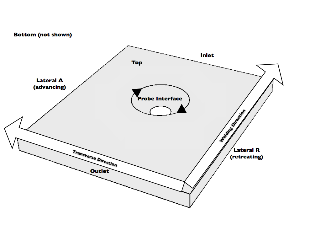
Figure 1: Surface designations for Eulerian domains used in the FSW simulations.

2.3 Governing Equations

A system of governing equations is specified to represent the thermomechanical response of the workpiece as a steady-state process. We do not model the transient response during either the probe insertion or the probe removal. The equations include balance laws for momentum, mass and energy, kinematic equations for the motion, constitutive equations for the material behavior, and boundary conditions. Altogether, the equations define spatial fields for the velocity, temperature and material strength. In the following subsections, we summarize the equations according to those used to determine each of the spatial fields and the numerical formulations for solving the respective sets of equations. The resulting systems are nonlinear and are solved numerically using a fixed point iteration procedure. The linear systems for each iterate of velocity and temperature were solved in parallel using the PETSc [10] library.

2.3.1 Equations governing the velocity field

Under the assumptions that viscous forces are much larger than inertial terms and that body forces may be neglected, balance of linear momentum reduces to

$$\operatorname{div}{\boldsymbol{\sigma}}=0\\$$ (1)

where ${\boldsymbol{\sigma}}$ is the Cauchy stress. From balance of angular momentum, the Cauchy stress is symmetric. The deviatoric Cauchy stress is determined from the deviatoric deformation rate, $\mathbf{D^{\prime}}$, through a viscoplastic constitutive law where the underlying flow is assumed to be incompressible and elastic strains are neglected. Under these assumptions

$$\boldsymbol{\sigma}^{\prime} = 2\mu\mathbf{D}^{\prime}$$

$$\operatorname{tr}{\mathbf{D}} = 0$$

The deformation rate is obtained from the velocity, $\mathbf{u}$, by

$$\mathbf{D}=\operatorname{symm}(\nabla\mathbf{u})$$ (2)

The effective viscosity, $\mu$ , is inferred from the relations for the rate-dependent flow stress of the material. We employ an empirical equation for the flow stress suggested by Kocks and Mecking [11]

$$\bar{\sigma}=\tau(s,\theta)f(\theta){\biggl{(}\frac{\bar{D}}{D_{0}}}\biggr{)}^{m(\theta)}$$ (3)

In this equation, the effective stress, $\bar{\sigma}$, is related to the effective deformation rate, $\bar{D}$, through a power-law dependence in which the deformation rate is normalized by a reference deformation rate, $D_{0}$. $\theta$ is the temperature. The exponent in the power-law relation is $m$, and is referred to as the rate-sensitivity. The effective stress and deformation rate are computed from the corresponding tensors according to $\bar{D}^{2}=\mathbf{D}^{\prime}:\mathbf{D}^{\prime}$ and $\bar{\sigma}^{2}=\boldsymbol{\sigma}^{\prime}:\boldsymbol{\sigma}^{\prime}$. There are two scaling terms for the flow stress: $\tau$ and $f$. $\tau$ is a function of the state variable for strength, $s$, and the temperature-dependent shear modulus, $G$. $f$ is a temperature-dependent term characterizing the activation energy. The specific forms of $\tau$ and $f$ are

$$\tau(s,\theta) = s\,G(\theta)$$

$$f(\theta) = \exp\biggl{(}\frac{Q}{R}\bigl{(}\frac{1}{\theta}-\frac{1}{\theta_{0}}\bigr{)}\biggr{)}$$

where $Q$ is the activation energy, $R$ is the universal gas constant, and $\theta_{0}$ is a reference temperature. Parameters $m$ and $G$ are linear functions of temperature

$$m(\theta) = m_{0}\,+m_{t}\theta$$

$$G(\theta) = G_{0}\,+G_{t}\theta$$

This model has two features that are particularly important to dealing with the wide range of strain rates and temperatures characteristic of friction stir welding simulations: the scaling of the flow stress by the temperature-dependent shear modulus and the explicit control of the rate sensitivity through the power law.

Boundary conditions are either specified velocity or traction components on each surface. The material contacting the probe is constrained to have zero velocity normal to the probe surface and a frictional traction that is applied tangentially to produce a desired torque. The weld speed is specified by specifying velocity of material entering the control volume at the inlet. Motions on the top, bottom and the two sides are also constrained to be tangential to those surfaces, respectively. Finally, the outlet has a zero traction everywhere.

2.3.2 Equations governing the temperature field

Balance of energy provides the governing equation for the temperature field, and may be written as

$$-\operatorname{div}(\kappa\nabla\theta)+\rho c_{p}\nabla\theta\cdot\mathbf{u}=\dot{\mathcal{Q}}$$ (4)

The first term quantifies heat transfer by conduction while the second quantifies advection. $\dot{\mathcal{Q}}$ is the heat generated in the body as a consequence of the viscous dissipation associated with the deformations ($\dot{\mathcal{Q}}=\boldsymbol{\sigma}^{\prime}:\mathbf{D}^{\prime}$). Material constants are the conductivity, $\kappa$, the mass density, $\rho$, and the heat capacity, $c_{p}$. All of these properties are functions of temperature.

Boundary conditions for the temperature field can be either a specified temperature or a heat flux. Several types of flux conditions are used. For convection and surface contact, the heat loss through a surface is linearly proportional to the difference in surface and ambient temperatures. For radiation, the flux is proportional, through the emissivity, to the fourth power of the difference in surface and far-field temperatures. The temperature is specified for the material entering the control volume at the inlet. The probe temperature is also specified using a value determined using the procedure detailed in Section 3. The top surface has a radiation condition, while the bottom surface has a heat flux due to contact with the anvil. The outlet has a zero (spatial) flux condition, but note that there is heat transfer across that boundary due to advection of mass exiting the control volume.

2.3.3 Equations governing the evolution of the state variable

The state variable, $s$, quantifies the strength and is a key part of the constitutive model discussed above. Again, we employ a model proposed by Kocks and Mecking [11]. Although this model was developed for face-center cubic polycrystalline materials, our experience is that it also works well for titanium, as well. The state variable is associated with a differential volume of material that may be taken as a point in the computational domain and evolves as a consequence of the deformation according to

$$\frac{Ds}{Dt}=\frac{h_{s}}{G(\theta)}(1-\frac{s}{s_{s}})^{n_{s}}\bar{D}\\$$ (5)

where

$$s_{s} = {\Biggl{(}a_{s}+b_{s}\biggl{(}\frac{{\tilde{\varphi}(\theta,\bar{D})}}{{\tilde{\varphi_{s}}}}\biggr{)}^{\frac{1}{2}}\Biggr{)}^{2}}$$ (6)

$$\tilde{\varphi}(\theta,\bar{D}) = \frac{\theta}{G(\theta)}\,ln\,\biggl{(}\frac{\mathit{D_{s}}}{\bar{D}}\biggr{)}$$ (7)

$$\tilde{\varphi}_{s} = {\tilde{\varphi}}(\theta_{r},\mathit{D_{r}})$$ (8)

Equation 5 gives the material derivative of $s$ in terms of the shear modulus, the effective deformation rate, the state saturation, $s_{s}$, and material parameters, $h_{s}$ and $n_{s}$. The state saturation is given in Equation 6 as a function of the Fisher factor, $\tilde{\varphi}$ (Equation 7). The Fisher factor is normalized by a reference value (Equation 8), namely the Fisher factor at a reference temperature and deformation rate, $\theta_{r}$ and $\mathit{D_{r}}$. The constants $a_{s}$ and $b_{s}$ are material parameters. For FSW applications, a critical feature of the evolution equation is the scaling of the state saturation with deformation rate and temperature. It is through the state saturation that bounds are imposed on the increases in flow stress from strain hardening/softening. Bounding the flow stress is central to maintaining realistic values of the computed stress and temperature over the large excursions of temperature and strain experienced in FSW.

For the state evolution, initial conditions are specified on the inlet surface. Equation 5 is integrated along streamlines of the flow field to determine how the state of material evolves as it passes through the control volume. For flows with recirculations (closed streamlines within the control volume), such as can occur on the probe surface, special treatment must be given. For points on a closed streamline, we assign the saturation value to the material state, as defined by Equation 6.

2.4 Numerical solution of the governing equations

The numerical solution of the governing equations proceeds as in [6]. For completeness, we include a brief statement of methodology used for each of the primary field variables (velocity, temperature and state variable).

The velocity field is determined from a weak form of the equilibrium equation:

$$-\int_{V}\boldsymbol{\sigma}:\nabla\,\boldsymbol{\Psi}\,{\rm dV}+\int_{S}\mathbf{t}\cdot\boldsymbol{\Psi}\,\mathit{dS}\,=\,0$$ (9)

where $\mathbf{\Psi}$ is a vector weighting function, $\mathit{V}$ is the workpiece volume, $\mathit{S}$ is its surface, and $\mathbf{t}$ is the surface traction. The viscoplastic constitutive equations for the flow stress are used to express the stress in terms of the deformation rate. The incompressibility constraint is enforced by a weighted residual as:

$$\int_{V}\,{\psi}\,\operatorname{div}\mathbf{u}\,dV\,=\,\int_{V}\,{\psi}\,{\operatorname{tr}(\mathbf{D})}\,dV\,=\,0$$ (10)

where ${\psi}$ is a scalar weighting function. This equation acts as a constraint on the motion allowed by Equation 9 and is treated by the consistent penalty method [12, 13].

To determine the temperature field, a residual is formed using the energy equation. Using the scalar weights, $\psi$, the residual may be written as:

$$\int_{V}\,[\operatorname{div}(\kappa\nabla\theta)-\rho c_{p}\mathbf{u}\,\cdot\,\nabla\theta\,+\dot{\mathcal{Q}}]\,\psi\,\mathit{dV}\,=\,0.$$ (11)

Streamline upwinding [14, 15] was used to stabilize the solution against spurious spatial oscillations.

We use the streamline integration method to solve for the material state variable at the nodal points. For steady flows, the material derivative in Equation 5 retains only the convective term

$$\frac{Ds}{Dt}=\mathbf{u}\cdot\nabla s$$ (12)

This allows the evolution equations for the state variable to be written along characteristic lines of the partial differential equation and integrated point-by-point as ordinary differential equations. To obtain the value of the state variable at a given node of the finite element mesh, we first trace the streamline passing through that node upstream to a point within the mesh where the state has already been evaluated. We use the value at that point as an initial condition for the evolution equation and then integrate forward to determine the value at the starting node. By progressing from the inlet to the outlet through the mesh, the distribution of state variable over the complete mesh may be determined efficiently [2, 3, 4].

3 Determining the Probe Boundary Conditions

To solve the governing equations, we need to specify values for the boundary conditions. For most surfaces on the workpiece, this is straightforward. However, values for the traction and temperature applied to the workpiece at the interface with the probe are problematic. Values for these quantities are particularly difficult to ascertain as this interface is not accessible to instrumentation. Here we present a methodology for estimating the local probe/workpiece interface conditions from experimentally known quantities associated with the probe, namely its translational and rotation rates and the resultant weld (probe) force and torque. Corresponding quantities can be computed from simulation data for specified tractions and temperature combinations applied to the workpiece/probe interface.

The methodology consists of adjusting the traction and temperature in a systematic way so that the simulated probe quantities come into agreement with measured values. To accomplish this, we make two simplifying assumptions regarding the distribution of frictional traction and interface temperature: both are uniform over the probe surface. Specifically, the applied traction is of constant magnitude and in the direction of rotation; it can derived directly from the measured torque. The applied temperature is uniform over the probe surface; its value can be derived indirectly from the weld force, given an accurate characterization of the dependence of the flow stress on strain rate and temperature. An iterative method is needed to identify the value of temperature for a particular mesh. The methodology delivers average interfacial frictional tractions and temperatures with resultants equal to those measured on the probe.

The simplicity of the boundary conditions enables a straight-forward check on the adequacy of the mesh to capture the true solution. The check is based on a comparison of the applied and recovered torques in the simulations. By repeating the simulations on meshes of increasing resolution, it is possible to confirm that the discretization error tends to zero and the solution converges to within an acceptable tolerance. We consider this error check to be a powerful tool in its own right and a central feature of our methodology in general. In addition, the error analysis revealed a key relationship between recovered values of torque and weld force in the FSW simulations, which we were able to exploit effectively in comparing simulation with experiments. Additional validation, independent of the values of probe traction and temperature, is provided by comparison of thermal fluxes with measured power consumption. Details are given below and in Section 4.

3.1 Resultants of Force, Torque, Heat Flux and Power

The resultant quantities of interest include the resultant forces, torques, heat fluxes and power. These are defined analytically as integrals of appropriate quantities over a particular surface or volume of interest. For a given finite element mesh, these integrals are integrated numerically using the approximate solution. The resultant force on a surface is the integral of the traction: $\int_{S}\mathbf{t}\>dS$, where $\mathbf{t}$ is the traction on surface $S$. When computed over the inlet surface, the resultant is the reaction needed to maintain equilibrium when the probe force is applied to the workpiece, and thus it corresponds to the weld force. The mechanical power on a surface due to a traction acting on material moving along the surface is computed by $\int_{S}\mathbf{t}\cdot\mathbf{u}\>dS$, where $\mathbf{u}$ is the velocity field on the surface; for the inlet surface, in particular, this is the weld power. The net heat flux crossing a surface is computed as $\int_{S}\mathbf{q}\cdot\mathbf{n}\;dS$, where $\mathbf{q}$ is the heat flux and $\mathbf{n}$ is the surface normal. If $\dot{\mathcal{Q}}$ is the heat generation density due to deformation, then the total heat generation rate over the body $V$ from mechanical dissipation is given by $\int_{V}\dot{\mathcal{Q}}\;dV$.

The torque calculation is of particular interest. The torque is the moment about the probe’s axis of rotation caused by the frictional tractions. The moment is computed as the integral over the probe surface of the vector cross product between the frictional traction $\mathbf{t}^{f}$ and its associated moment arm about the probe axis. We represent the probe axis of rotation using a point $\mathbf{p}$ on the axis and a (unit vector) direction $\mathbf{a}$. For a point $\mathbf{x}$ on the surface, the moment arm $\mathbf{r}$ is the vector connecting the axis at point $\mathbf{p}$ to the point of application: $\mathbf{r}$ = $\mathbf{x}-\mathbf{p}$. To obtain the torque about the rotation axis, we take the component of the moment aligned with $\mathbf{a}$, resulting in a scalar value for the torque. Thus, the resultant torque $T$ about the probe axis of rotation from the action of the frictional tractions on the probe surface is given by

$$T=\mathbf{a}\cdot\int_{S}\mathbf{r}\times\mathbf{t}^{f}\;dS$$ (13)

3.2 Estimation using force and torque resultants

The full procedure for determine boundary values to apply on the probe interface involves solving the finite element systems on two or more meshes. By proceeding from coarser to finer meshes, it is possible to estimate resultants on more finely resolved meshes from analysis of error associated with individual meshes. In this section, we describe the complete process beginning with the determination of the traction and temperature for a single, fixed mesh.

3.2.1 Traction and temperature for a fixed mesh

The basic procedure of the methodology is to find a traction and a temperature for the probe interface that will give resultants for probe torque and weld force that are equal to the measured values. The traction value is determined by computing the torque assuming a unit traction in Equation 13 and rescaling it to match the desired value of torque, i.e. the measurement. The temperature is found indirectly by determining the probe temperature that leads to a computed weld force that is equal to the measured weld force. This procedure involves finding the solutions for several possible probe temperatures and from these estimating the temperature that will provide the best match between measured and computed weld force. We note here that the weld force that is recovered from each solution will be adjusted based on the estimated error (described below), and that adjusted value will be used for comparison with the measured weld force. In the FSW system, when the assumed probe temperature increases, the recovered weld force decreases. By solving the FEM equations with different assumed probe temperatures and computing the associated weld forces, one can quickly narrow the range of probe temperatures that provide reasonable weld forces. Our experience is that this iteration converges quickly and only a handful of systems need to be solved. In the end, we obtain a temperature and a traction to apply on the probe interface which are consistent the measured torque and weld force.

3.2.2 Estimation of error for a fixed mesh

The procedure outlined in Section 3.2.1 provides values for probe traction and temperature for which the simulation results match target values for torque and force for a specified mesh. This process does guarantee that the solution using that mesh is otherwise accurate, however. To make that assessment the discretization error associated with the mesh must be estimated. Because we use a uniform traction condition on the probe interface, we have a natural check on the quality of our solution. After a solution is computed for a given mesh and set of boundary conditions, it is postprocessed to compute macroscopic resultants, including the torque. In this computation, the internal stresses are evaluated at the points on the boundary from the deformation rate and temperature using the constitutive equations. If the solution estimates either of these poorly at critical points, then the stress will be poorly estimated at those points as well. The consequence here is that the torque recovered from the internal stress may not match the torque applied externally via the boundary conditions. Thus, we use a comparison of the recovered torque to the applied torque to determine the magnitude of the discretization error in the deformation rate and temperature and the need for additional mesh refinement.

Additionally, for the particular models used in this paper, we found and exploited a relationship between the error in the torque and the recovered weld force. The recovered torque was too low in each case, with the finer results being closer to, but still below, the target value. Meanwhile, the recovered weld force decreased with finer mesh resolution, meaning that the estimate for weld force from any given mesh was consistently too high. This trend applied to all the cases we considered in the application presented in Section 4. The error in the recovered torque and the error in the estimate of the weld force correlate as both stem from the discretization of the workpiece. Consequently, it is possible to compute a better estimate of the weld force by adjusting the computed weld force using a factor proportional to the torque error. Equation 14 gives the formula for the weld force adjustment, where $f_{\rm adj}$ is the adjusted weld force, $E$ is the relative (proportional) error in the torque, and $f_{\rm rec}$ is the recovered resultant weld force from the simulation

$$f_{\rm adj}=(1-E)f_{\rm rec}$$ (14)

The adjustment to the computed weld force removes most of the effect of mesh size, providing a consistent value across meshes. This is what we use in our comparisons in Section 4.

3.2.3 Reduction of error by mesh refinement

The procedure for a single fixed mesh is repeated on meshes with greater resolution until the solution has converged to within a specified tolerance. The discrepancy between the torque recovered by postprocessing and the torque used to compute the applied friction traction serves as a effective measure of the convergence of the entire solution. By repeating the procedure described above on different meshes, one can check that the solution is converging by monitoring the discrepancy in torques. To make this quantitative, we need to prescribe a measure of the element size, commonly referred to using the variable $h$. Here, we use $h=\sqrt[3]{1/n}$, where $n$ is the number of nodes in the mesh. While our meshes are not perfectly regular, they are based on sections with regular subdivisions, so this is roughly proportional to the element size. In section 4, our errors in traction will be seen to have a very strong linear convergence with $h$.

3.3 Validation using power resultants

Finally, other measured resultants should be compared with the recovered values. The thermal resultants are of particular interest because we used the mechanical resultants to calibrate the probe traction and temperature. One resultant we have available for comparison is the total power used to rotate the probe. which is computed from the product of the rotation rate and the measured torque. However, we do not know the partitioning of the power between the workpiece, the tooling, and the environment. Still, the total power provides an upper bound on the amount of heat generated. For our application, the solution approaches this limit with increasing translational speed, indicating a greater fraction of the total power is transferred to the workpiece as the probe translation rate increases.

4 Application to FSW of Ti5111

We illustrate the methodology to determine probe interface boundary conditions from knowledge of the force and torque applied to the probe via the tooling on an example of friction stir welding of a titanium alloy. Process parameters include weld speed, rotation speed, probe and workpiece geometries, as well as material properties. The mechanical properties are taken from published values or from fitting of model constants to published data.

4.1 Experimental Data

The process data comes from FSW experiments described in greater detail in [16] and summarized briefly here. Three welds were performed on quarter-inch sheet made of the titanium alloy, Ti-5Al-1Sn-1Zr-0.8Mo (Ti5111). All three welds were made at the same probe rotational speed of 225 rpm, but at different weld speeds: a slow speed of 1.0 ipm (inches/minute), a medium speed of 2.5 ipm, and a fast speed of 4.0 ipm. The data include weld force profiles, from which we took nominal values of 31 kN, 36 kN and 38 kN for the slow, medium and fast weld speeds, respectively. The torque was not measured independently for all weld speeds, but a nominal value of 47 Nm was provided for all three cases. As a check, we can compute the rate of power input from the torque and rotation speed, giving approximately 1,100 W; the power contribution from the forward movement of the probe is much less, but increases with weld speed. This data set lacks detailed information on heat loss through the probe via controlled cooling and so only a partial check on the partitioning of input power is possible. Microstructures and textures for these welds are examined in [17].

Parameters for the thermal and mechanical constitutive models summarized in Section 2 were estimated from available data in the literature [18]. For the Kocks-Mecking model, the parameters were found by fitting to data from the [19] for Ti64. These data were used as a reasonable representation of the Ti5111 behavior in the absence of adequate data for Ti5111 itself. Values of the model parameters are given in Table 1. In [20], experimental thermocouple data for Ti64, indicated that stir zone temperatures exceed the beta transus. To allow for the change of phase, we use two sets of parameters for the two regimes. One set applies to the higher temperature BCC phase, the other set to the lower temperature HCP phase. The thermal properties, however, were taken as the same for both phases.

Table 1: Material parameters used in simulations.

parameter	unit	phase 1	phase 2
Flow Properties
$G_{0}$	GPa	43.4	43.4
$G_{t}$	GPa/K	-0.021	-0.021
$m_{0}$	-	0.05	-0.685
$m_{t}$	1/K	0.0	0.0007
$Q/R$	K	100.0	1000
$\theta_{0}$	K	462.0	900.0
$D_{0}$	1/s	1.0	1.0
State Evolution
$a_{s}$	-	0.17	0.304
$b_{s}$	-	-0.02	-0.185
$h_{s}$	GPa	50.0	20.0
$n_{s}$	-	1.0	1.0
$D_{s}$	1/s	$10^{7}$	$10^{7}$
$\theta_{r}$	K	1150	1150
$D_{r}$	1/s	1.0	1.0
Thermal Properties
$\rho$	kg/$\mbox{{m}}^{3}$	4430
$c_{p}$	J/kg K	533
$\kappa$	W/mK	7.5

As discussed in Section 2, of particular interest is the saturation stress, which appears in the evolution equation for the strength and is a function of temperature and strain rate. The saturation stress bounds the flow stress in the limit of large strain deformations and serves to prevent the computed stresses from becoming unrealistically high as a consequence of the large strains imposed on the material as it passes close to the probe. The saturation stress as a function of normalized Fisher factor is shown in Figure 2 based on flow stress data reported for Ti64 [19]. Also shown are the computed stress-strain histories for simulated tensile tests corresponding to a range of strain-rate and temperature combinations. Note that under the assumed starting state, many of the responses demonstrate softening (a reduction of flow stress) as deformation heating raises the material temperature, which in turn lowers the saturation stress.

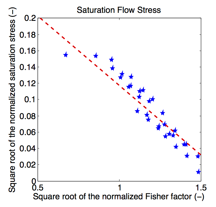
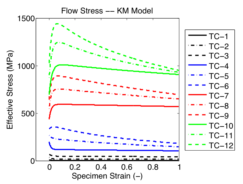
Figure 2: Computed stress strain curves for polycrystalline Ti5111 using the Kocks-Mecking model. Caption labels indicate test strain rate and temperature $(\bar{D}(1/s),\theta(K))$ according to: TC-1=(0.01,1273); TC-2=(1.0,1273); TC-3=(25,1273); TC-4=(0.01,1073); TC-5=(1.0,1073); TC-6=(25,1073); TC-7=(0.01,673); TC-8=(1.0,673); TC-9=(25,673); TC-10=(0.01,273); TC-11=(1.0,273); TC-12=(25,273);

4.2 Simulation Geometry

The model geometry from Figure 1 is shown in Figure 3 with the finest mesh discretization used in the simulations discussed here. The domain width was 120.2 mm; the length of the region ahead of the probe was 60.1 mm, and the length behind the probe was 72.75 mm. The domain is extended downstream of the pin (one additional probe length) to better capture the lateral gradients in the temperature field. The probe shape was a truncated cone with diameter of 12.65 mm at the top and 4.65 mm at the bottom. No shoulder is used in this model, consistent with the experimental conditions.

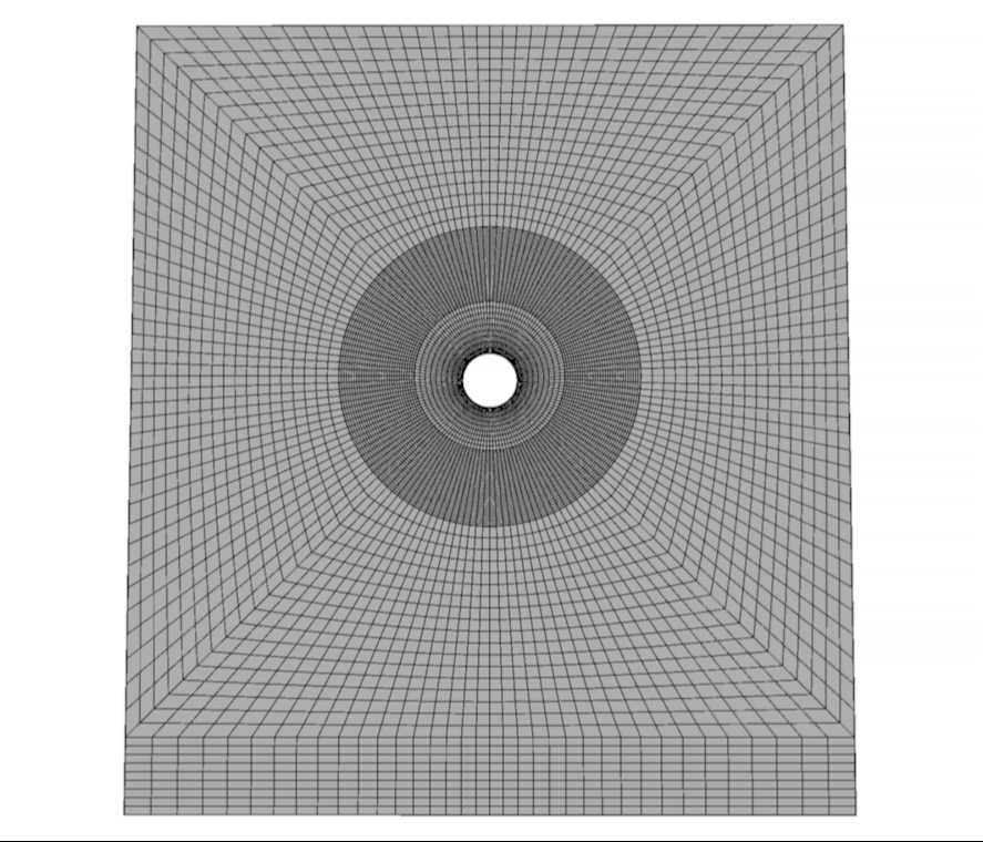
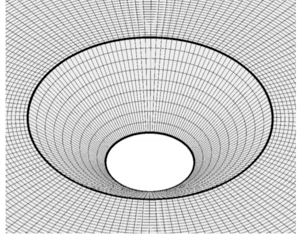
Figure 3: Simulation geometry: (left) view from above, (right) close-up view from above of the probe surface discretization.

Three meshes, using 20-node brick elements, were used. Mesh A was the coarsest, having 5,376 elements and 26,488 nodes. Mesh B was a direct refinement of Mesh A, having twice the resolution in every direction; it had 43,008 elements and 191,696 nodes. Mesh C had the finest resolution and was used for the final results; it had 65,124 elements and 286,641 nodes.

4.3 Probe Interface Boundary Conditions

The procedure to determine boundary values for the probe interface was described in Section 3. We applied this procedure for each of the three experimental cases with different weld speeds. The methodology begins with estimation of the probe traction and temperature on the coarsest mesh, Mesh A. The probe traction is computed directly from the known value of the torque using Equation 13. The measured data indicated the torque was approximately the same for all three weld speeds. For the probe geometry used here, a probe traction of 9.23 MPa produces the measured torque value of 47 Nm. Using this traction for all three weld speeds, we ran several simulations spanning a range of assumed probe temperatures. The simulation results were postprocessed to obtain the various resultant quantities of interest, with the recovered torque and force for the slowest weld speed shown in Figure 4. The torque and force both decrease with probe temperature over the range in probe temperatures from 1380K to 1400K (for the slowest case). For the torque, the error in the recovered torque ranges from 10% in the slow case to nearly 40% in the fast case. As described in Section 3, the recovered weld forces were adjusted based on the error in the recovered torque. Based on the trends illustrated in Figure 4, the target weld force of 31 kN is achieved using a probe temperature of 1390 K for the slowest weld speed of 1 ipm. The probe temperatures for the 2.5 and 4 ipm for Mesh A were 1470 K and 1530 K, respectively.

To reduce the discretization error, the simulations were repeated with Mesh B, which has twice the resolution of Mesh A in all directions, using the same input parameters. For comparison, the recovered resultants for this mesh are also shown on Figure 4. The recovered torque and force both move closer to their respective target values. The torque errors of Mesh B were very nearly half those of Mesh A, indicating a linear convergence with mesh size. Note also that the adjusted weld forces for the two meshes are nearly the same over the entire range of probe interface temperature. This indicates that the adjustment, based on the estimated error in torque, removes a primary effect of mesh size, allowing a consistent estimation of weld force independent of the mesh. A final simulation was done for Mesh C at the optimal temperature suggested by the analyses on Meshes A and B. After postprocessing to obtain the resultants, the same adjusted weld force was obtained.

Figure 5 summarizes the weld force results at the optimal temperature for all three weld speeds and all three meshes. Mesh results are shown from top to bottom, corresponding to finest to coarsest mesh resolution. For each mesh, three bars are shown: the recovered weld force in light gray, the adjusted weld force in darker gray, and the target value in black. The optimal temperature for the medium weld speed was 1470 K; for the fast weld speed, it was 1530 K. Note that the optimal temperatures for the finest mesh were the same as those found for the coarsest mesh. Thus, by using the adjusted weld force, we found consistent probe temperatures for all three weld speeds.

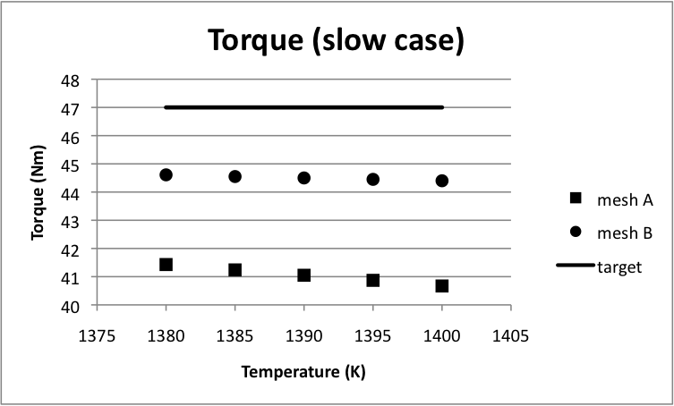
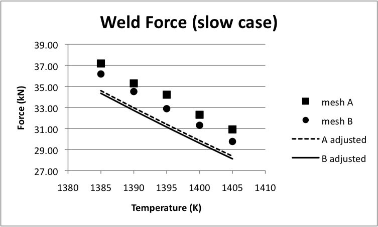
Figure 4: Relation of torque error to computed weld force for two mesh resolutions, including adjusted weld force.

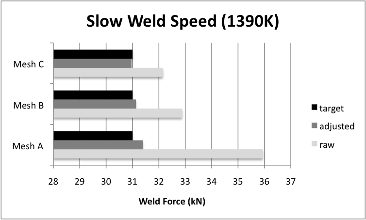
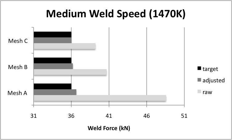
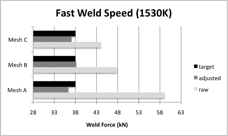
Figure 5: Weld force results at optimal temperatures for all weld speeds. Plots show recovered, adjusted and target weld forces for each of three meshes.

As a final check, we compared the power usage with the empirical data. The empirical data gives a constant torque of 47 Nm and a constant rotation speed of 225 rpm for all three weld speeds. Those values correspond to a constant energy input from the tool rotation of 1118 W; a much smaller energy input comes from the linear motion of the tool. The information we do not have, however, is how much energy is removed by cooling of the tool. In our study, higher tool temperatures were required for the simulation weld force to match the experimental weld force at higher weld speeds. Specifying a higher probe temperature in the simulation results in higher flux across the probe-workpiece interface and greater heat input into the workpiece. However, more material moves past the probe with higher weld speed, resulting in this application with the heat input per unit length of weld decreasing with increasing weld speed. Nevertheless, the fraction of the total heat input being deposited in the workpiece increases with increasing weld speed, approaching the entire input for the highest weld speed of 4 ipm. The power usage, including both frictional heating and mechanical deformation heating, is shown in Table 2. All these numbers fall well within the empirical range. The slower cases indicate significant heat loss to the environment or through cooling. The energy per unit length is generally of interest and is also given in the table.

Table 2: Power Usage

Weld Speed	Probe Heating Rate	Heat per Weld Length
(in/min)	(W)	(J/mm)
1.0	396	966
2.5	696	694
4.0	977	615

4.4 Influence of Torque

As stated in Section 4.1, the data set includes only an estimate of the nominal torque, which is the same for all speeds. To study the sensitivity of the probe temperature to torque variations, we repeated the suite of simulations for two values of applied traction other than the empirical value of 9.23 MPa. Values of 6.0 MPa and 12.0 MPa were assumed, which were estimated from experience to bracket the actual values of torque. The results for the slow weld speed are shown in Figure 6. Three plots are presented, one for each value of applied traction. Each plot shows weld forces as a function of five temperatures ranging from 1385 K to 1405 K. For each temperature, four values are shown: the recovered weld force and the adjusted weld force, based on torque error, for both Mesh A and Mesh B. The adjusted weld forces align to within 1% in all three cases. Also shown in each plot is a horizontal line indicating the empirical weld force of 31 kN. The probe temperature is taken to be where the target line intersects the line of adjusted weld force.

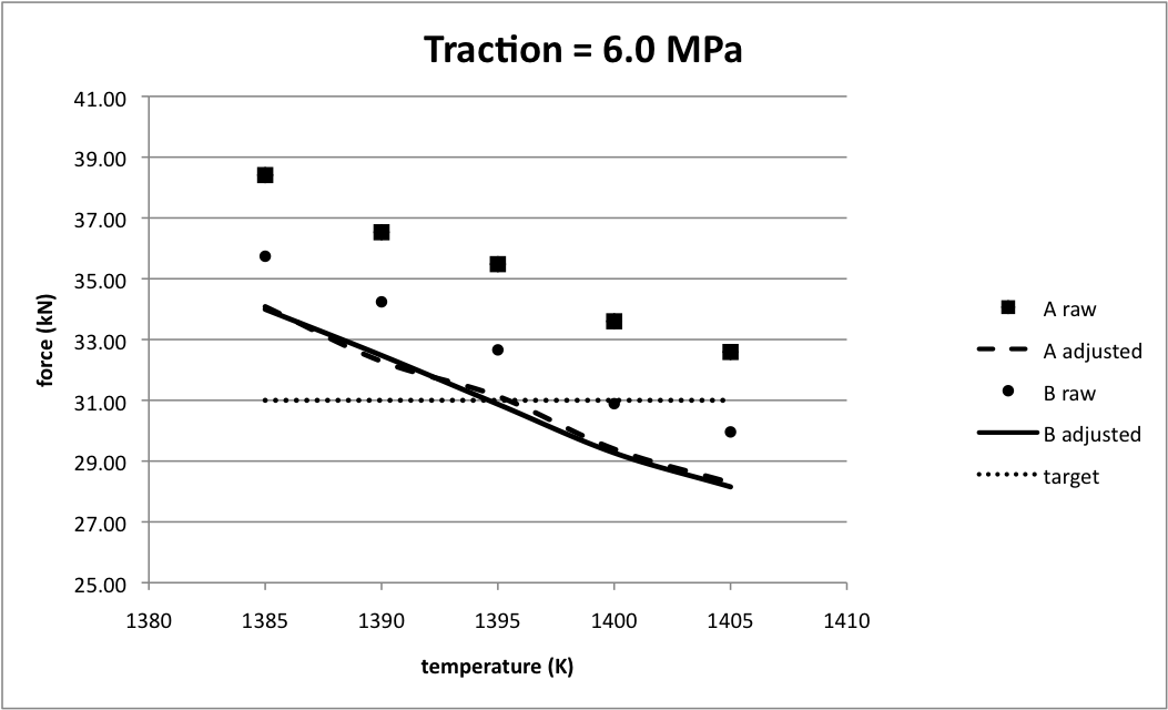
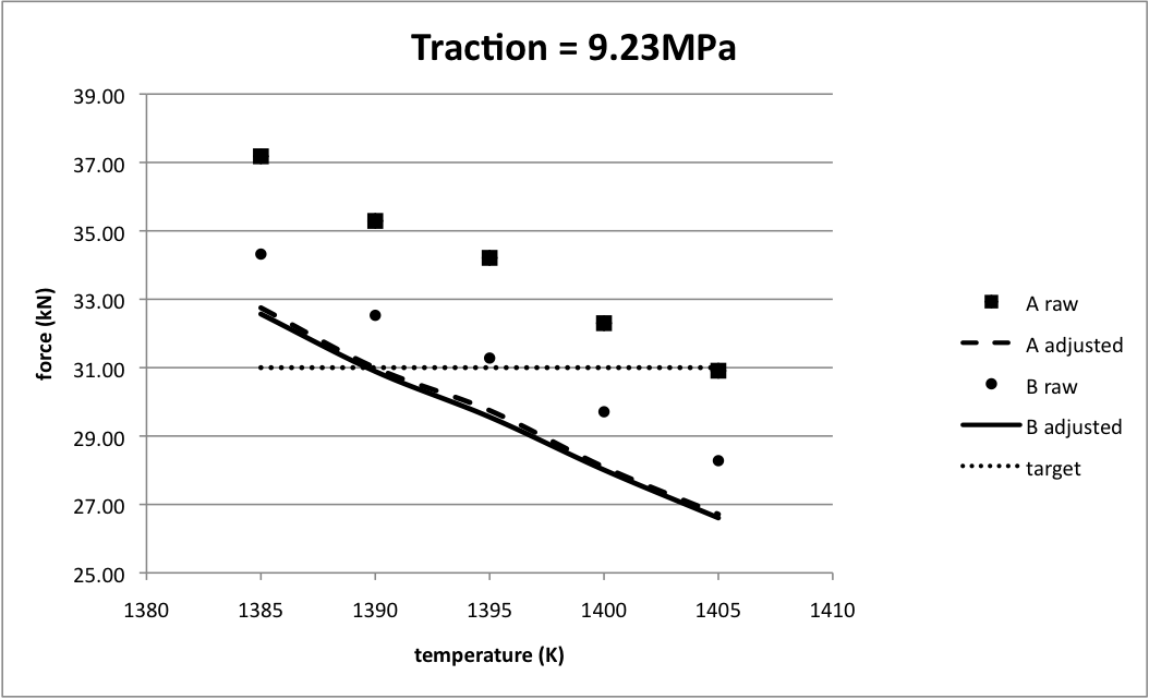
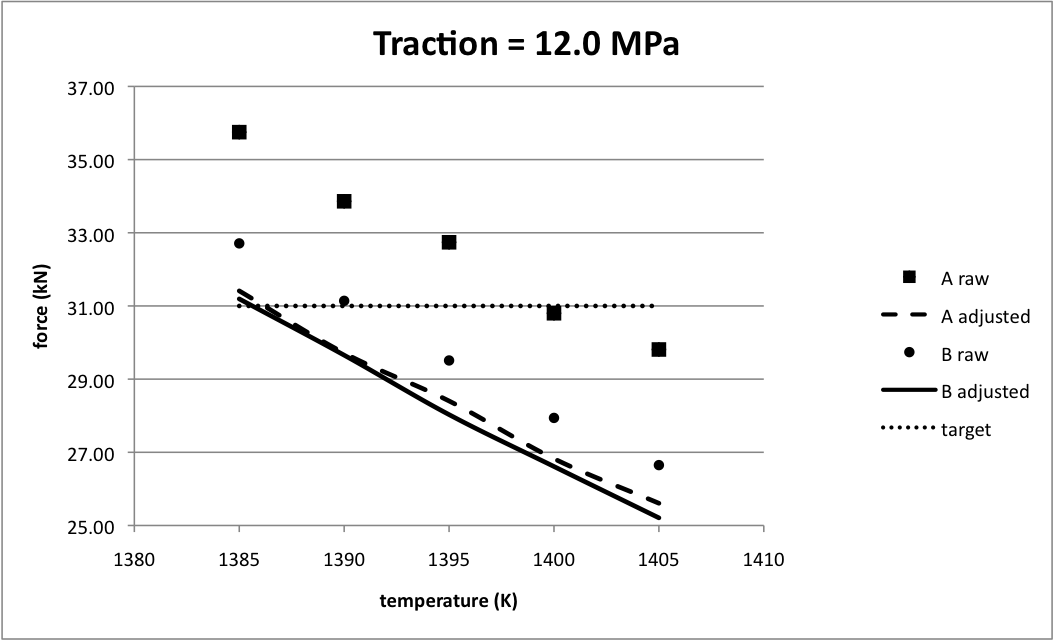
Figure 6: Weld force and temperature for two meshes and three values of torque.

The sensitivity of the probe temperature to changes in torque is small. For the slow weld speed, as the applied torque doubles, the probe temperature required to produce the same weld force varies by only 10 K, going from 1395 K down to 1385 K. The two cases of faster weld speeds produced very similar results.

5 Field Quantities

In FSW, friction between the probe and the workpiece acts to heat and shear the material in the vicinity of the probe. The elevation of temperature upstream of the probe lowers the flow stress and makes it possible to advance the probe with reasonably low forces. With the proper welding parameters, the ductility is adequate to accommodate the large shear strains without inducing unacceptable levels of damage. The simulations provide coupled solutions to the mechanical, thermal, and state evolution problems, as described in Section 2. Each of these problems involves aspects of the material’s response during FSW that bears on the quality of the weld. Having generated solutions that match the empirical data and that are adequately converged, we can examine those solutions for insight into how the process deforms, heats and alters the material.

5.1 Thermomechanical response

The primary variable of the mechanical problem is the velocity field. Material enters the control volume and flows past the probe. Material in the path of the probe is drawn around the probe preferentially in one direction by the frictional tractions of the rotating probe. This occurs in a relatively thin deformation zone in close proximity to the probe surface as can be seen from streamlines of the flow field shown in Figures 7. It may also be observed that there is a point upstream of the probe on the advancing side where the flow splits into the part that passes the probe on the retreating side and the part that passes the probe on the advancing side.

The weld speed has a clear influence on the overall flow pattern. For the slow case, the streamlines are nearly symmetric ahead of and behind the probe. As the weld speed increases, the material is pulled more strongly to the advancing side, and the flow also becomes more three-dimensional. For the fast case, there is a strong deformation zone behind the probe on the advancing side where the separated material is being rejoined.

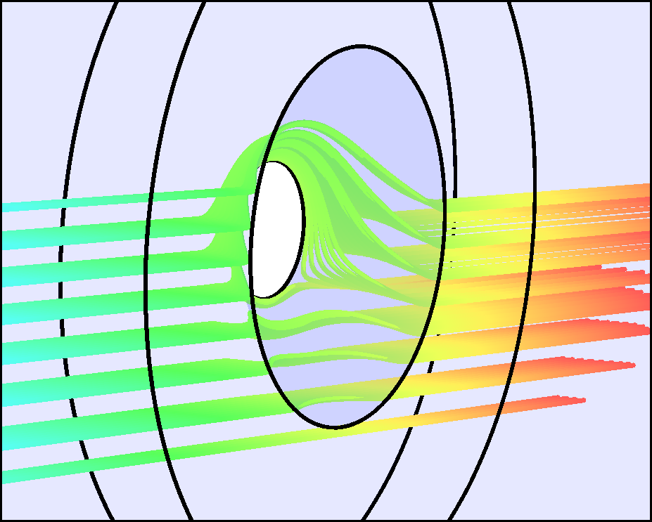
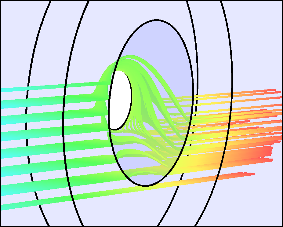
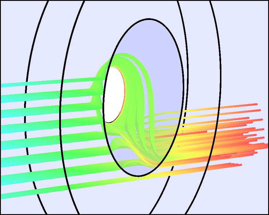
Figure 7: Streamlines illustrating flow pattern: slow and medium on top, fast on bottom. Color shows residence time.

Because of the highly coupled nature of the temperature and velocity, we shown distributions of temperature, deformation rate and effective stress together in Figure 8. The temperature profile is similar in shape for all three weld speeds, but narrows with increasing weld speed as the material behind the probe spends less time near the heat source. In general, the stress and deformation rate display some similarities, but due to the nonlinear, temperature-dependent behavior specified by Equation 3, they are not directly proportional to each other. Upstream of the probe, high values of the effective strain rate are limited to a narrow zone quite close to the probe surface. Downstream of the probe, the zone widens, reflecting the reduced rate sensitivity in Equation 3 at higher temperature. The effective stress is largest directly upstream of the probe. This is mainly a consequence of the probe pressing against the material under the action of the welding force. The material must deform to flow around the probe, which requires a higher level of stress upstream where material is just being heated. Downstream of the probe, the effective stress is substantially lower than upstream for two reasons. First, the material is at elevated temperatures and, second, the strength has been reduced (as is discussed in Section 5.2). Note that the applied frictional traction on the probe is substantially smaller than the peak values of the effective stress. This indicates that the forces necessary to induce plastic flow of the workpiece are coming primarily from the normal tractions along the probe, which are associated with the weld force rather than the torque.

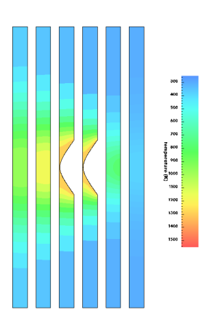
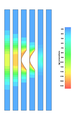
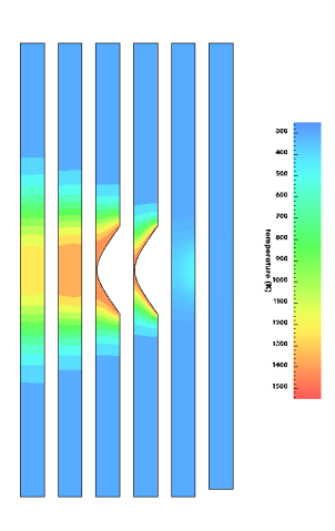
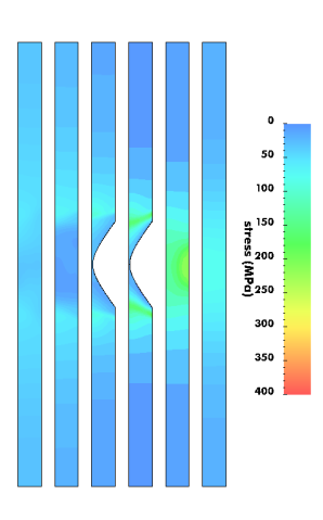
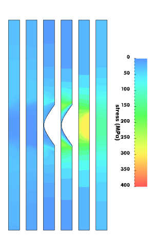
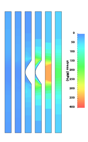
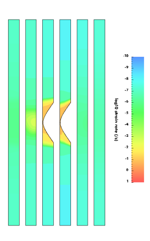
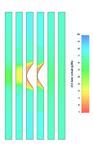
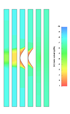
Figure 8: Temperature (top), effective stress (center), and strain rate(bottom, log scale) for increasing weld speed from left to right. For each field, slices perpendicular to the weld direction are shown from the inlet on the right to the outlet on the left.

5.2 Evolution of the Strength

Contour plots of the material state variable are shown in Figure 9. The material thermally softens immediately near the probe quickly reaches a steady value dictated by the saturation stress. The contour plots are qualitatively similar for all weld speeds. Cross sections on the outlet are shown in Figure 9. These images represent the material state after welding, but before possible thermal recovery. The state variable has a large, softened region in the middle, which would empirically be called the weld nugget. Bordering the nugget is a transition region characterized by a sharp gradient in the state. Beyond the transition zone is base material in which the state is unchanged. The contours in this transition zone sharpen with increasing weld speed, likely due to the narrowing band of heating behind the probe.

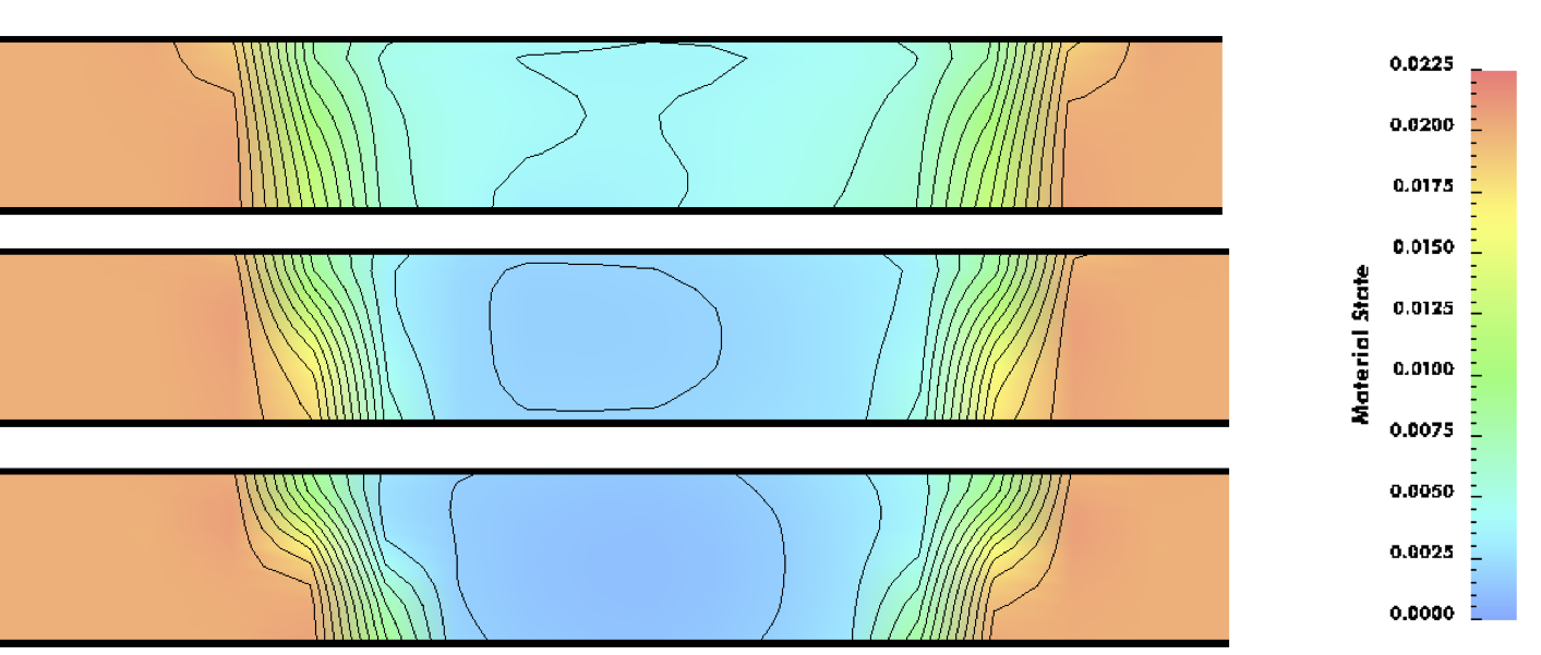
Figure 9: Material state cross-sections by weld speed (increasing from top to bottom).

5.3 Streamline Histories

The field plots presented in Figures 8 and 9 give spatial distributions of thermal and mechanical variables. It is often of interest to quantify the thermomechanical histories of material differential volumes (material points) throughout the FSW process. Such information gives the processing path experienced by material points from different zones in the workpiece. These data can be used for direct comparison to embedded thermocouple records, to verify if flow stress data encompasses the process conditions, or as input to microstructural models, for example. Figure 10 illustrates a collection of thermomechanical records for a set of material points originally along the centerline of the weld. One can see that the material is heated rapidly as it nears the probe. It begins intensive straining prior to being swept around the probe, and continues to deform until it is just downstream of the probe. The action of the probe compresses the material in the weld direction while stretching it in the transverse direction. The combination of high temperature and deformation reduces the strength as material approaches the probe, dropping the flow stress. In contrast to the strain rate, the stress peaks further upstream of probe. In this region, the influences of thermal softening and strength recovery, has not yet reduced the flow stress as it does later in the process.

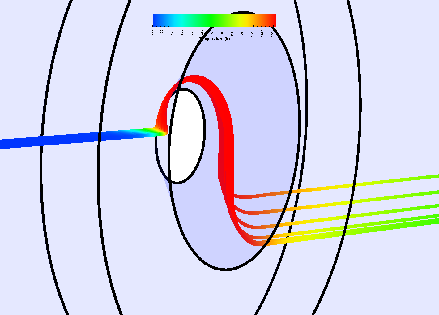
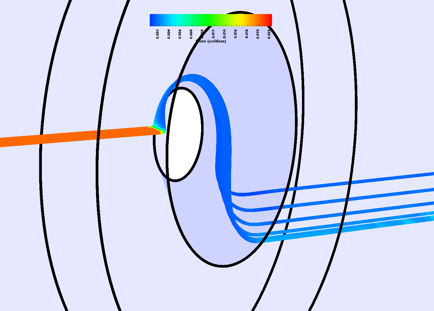
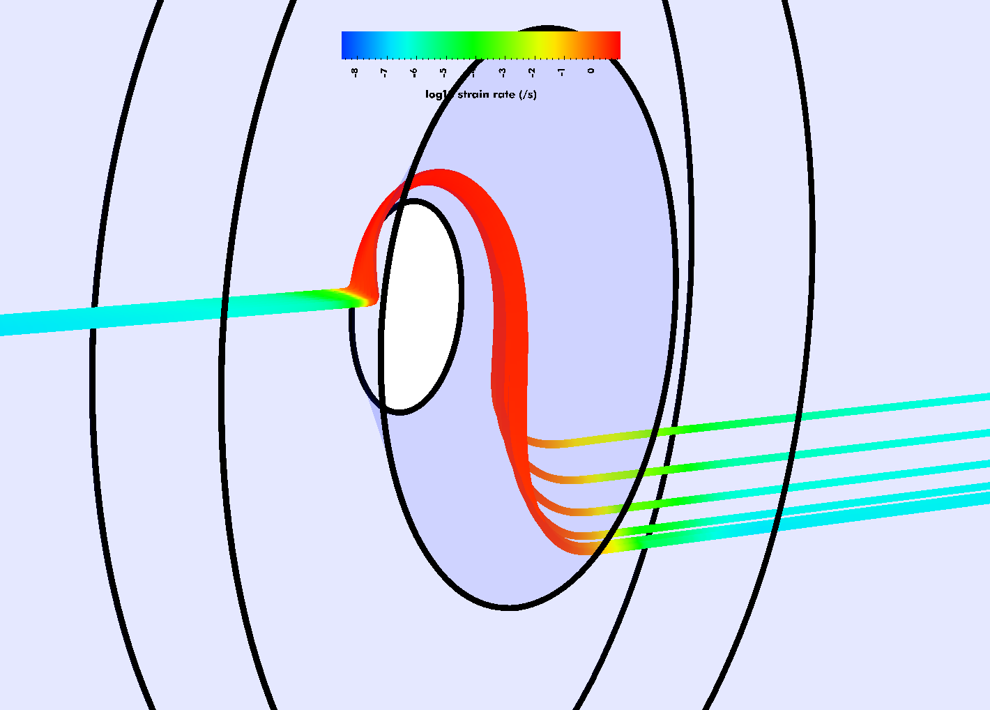
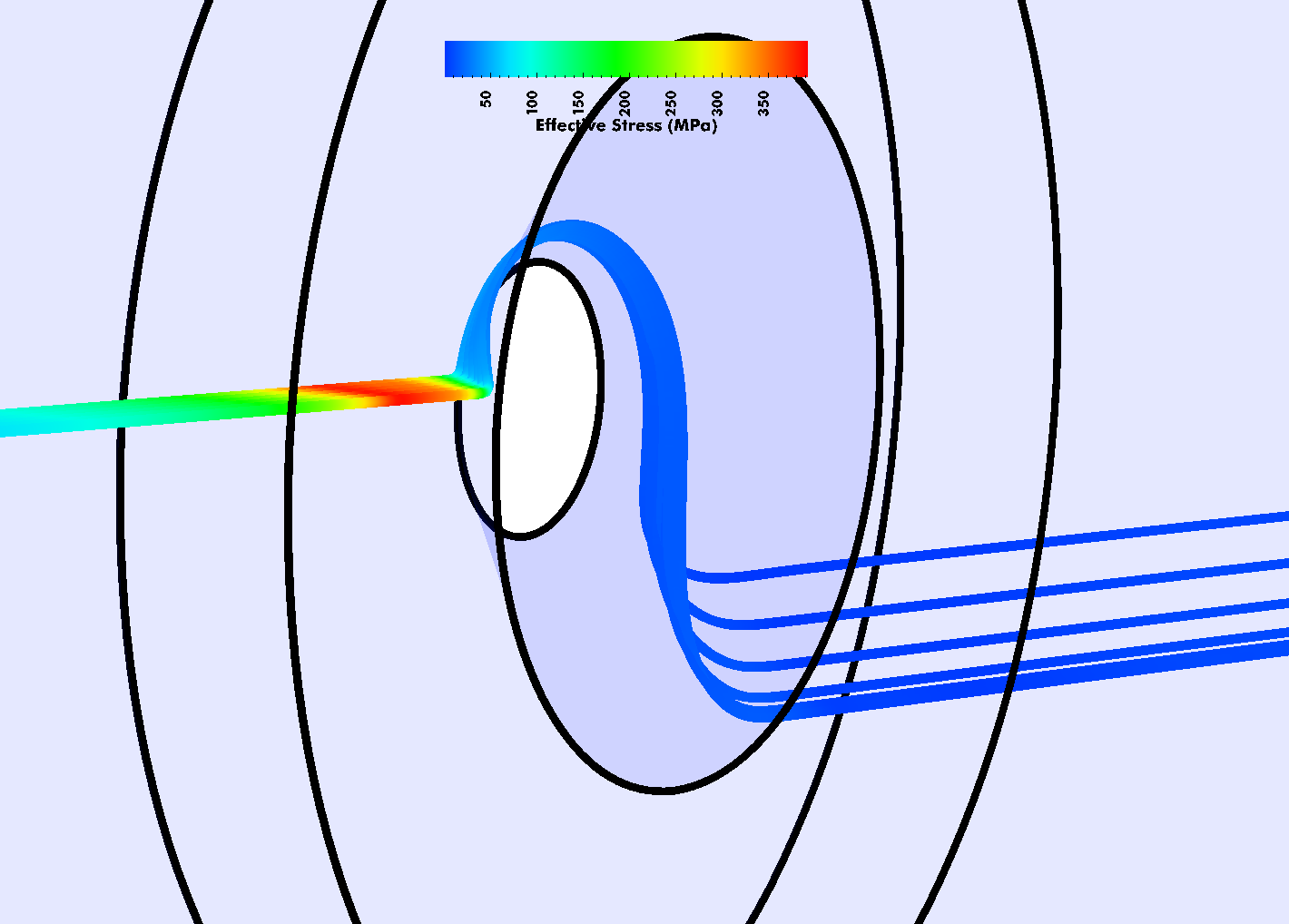
Figure 10: Data fields for fast case shown along streamlines. Top row: temperature and state. Bottom row: deformation rate and stress.

6 Summary

In this work, we developed a methodology to determine values for temperature and traction on the probe interface in finite element simulations of friction stir welding. The methodology goes beyond simple evaluation of boundary values and includes verification of mesh convergence and estimation of the error. We applied the methodology to model an experiment involving Ti5111 under three different weld speeds. For each of the three cases, we calibrated our boundary values using resultant weld forces and torques. The simulation results were consistent with empirical power measurements, the resulting data fields were discussed.

The boundary conditions are of the simplest form—we use a constant traction derived directly from the measured torque and a constant temperature derived indirectly through its relation to weld force. The traction magnitude is computed analytically from the geometry of the probe surface, given the measured value torque. The calculation of the probe temperature is indirect and requires a few simulations. Essential to the success of the method is a high quality material model that captures the material’s thermal softening with temperature. The temperature on the probe interface is varied until the measured weld force is attained. In the end, the values of temperature and weld force are consistent with measured resultants of torque and weld force, and any other available data can be used for validation.

We ran the simulations on multiple meshes to evaluate the discretization error and to assure that the solution was converged. The recovered torque, the value obtained by postprocessing the simulation result, was compared with the analytically expected value and used as an estimate of error. For the examples shown, the estimated errors decreased as expected with the mesh size. Furthermore, we were able to use the estimated error in the torque to predict converged weld forces. That allowed us to obtain consistent trends for the probe temperature across all meshes.

Our simulations modeled friction stir welding of Ti5111 at three weld speeds. The power usage was within bounds dictated by the experimental conditions, and the simulations indicated significant cooling through the tool. After plotting the data fields, a consistent picture of the stir welding process emerged. The primary effect of the stirring is to heat the material ahead of the probe in order to soften it sufficiently for the probe to advance though the material. The peak stresses occur as the probe approaches, due to the compressive action of the welding force on material that is not yet fully heated. Once the material is drawn around the probe, it heats rapidly. The faster weld speeds showed greater lateral spread in the flow, with more vertical mixing.

References

- [1] T. Belytschko, W. K. Liu, and B. Moran. Nonlinear Finite Elements for Continua and Structures. John Wiley and Sons, 2000.
- [2] P. R. Dawson. A model for the hot or warm working of metals with special use of deformation mechanism maps. International Journal of Mechanical Sciences, 26(4):227 – 224, 1984.
- [3] A. Agrawal and P. R. Dawson. A comparison of Galerkin and streamline techniques for integrating strains from an Eulerian flow field. International Journal for Numerical Methods in Engineering, 21:853 – 881, 1985.
- [4] P. R. Dawson. On modeling of mechanical property changes during flat rolling of aluminum. International Journal of Solids and Structures, 23(7):947–968, 1987.
- [5] Jae-Hyung Cho, Donald E. Boyce, and Paul R. Dawson. Modeling strain hardening and texture evolution in friction stir welding of stainless steel. Materials Science and Engineering A, 398:146–163, May 2005.
- [6] J-H Cho, D E Boyce, and P R Dawson. Modelling of strain hardening during friction stir welding of stainless steel. Modelling and Simulation in Materials Science and Engineering, 15(5):469–486, 2007.
- [7] B. Liechty and B. Webb. Modeling the frictional boundary condition in friction stir welding. International Journal of Machine Tools and Manufacture, 48(12-13):1474–1485, October 2008.
- [8] M. Ainsworth and J. Tinsley Odin. A posteriori error estimation in finite element analysis. Computer Methods in Applied Mechanics and Engineering, 142(1-2):1–88, March 1997.
- [9] Rudiger Verfurth. A Review of Posteriori Error Estimation & Adaptive Mesh-Refinement Techniques. John Wiley & Sons, May 1996.
- [10] S. Balay, K. Buschelman, W. Gropp, D. Kaushik, M. Knepley, L.C. McInnes, B. Smith, and H. Zhang. PETSc Users Manual. Argonne National Lab., 2002. (Argonne, IL, US).
- [11] U. Kocks and H. Mecking. Physics and phenomenology of strain hardening: the FCC case. Progress in Materials Science, 48(3):171–273, 2003.
- [12] M.S. Engelman, R.L. Sani, P.M. Gresho, and M. Bercovier. Consistent versus reduced integration penalty methods for incompressible media using several old and new elements. International Journal for Numerical Methods in Fluids, 2:25–42, 1982.
- [13] Y.S. Lee and P.R. Dawson. Obtaining residual stresses in metal forming after neglecting elasticity on loading. Journal of Applied Mechanics, 56(6):318–327, 1989.
- [14] T. Belytschko, W.K. Liu, and B. Moran. Nonlinear Finite Elements for Continua and Structures. JOHN WILEY & SONS LTD, 2000. chap. 7.
- [15] A. Brooks and T. Hughes. Streamline upwind/Petrov-Galerkin formulations for convection dominated flows with particular emphasis on the incompressible Navier-Stokes equations. Computer Methods in Applied Mechanics and Engineering, 32(1-3):199–259, September 1982.
- [16] Jennifer N. Wolk. Microstructural Evolution in Friction Stir Welding of Ti 5111. PhD thesis, University of Maryland, 2010.
- [17] R. W. Fonda and K. E. Knipling. Texture development in near-ΠTi friction stir welds. Acta Materialia, September 2010.
- [18] H. E. Boyer and T. L. Gall, editors. Metals Handbook. ASM International, 1985.
- [19] P. K. Chaudhury and D. Zhao. Atlas of formability: Ti-6Al-4V ELI. Technical report, National Center for Excellence in Metalworking Technology, 1992.
- [20] A. Pilchak, W. Tang, H. Sahiner, A. Reynolds, and J. Williams. Microstructure Evolution during Friction Stir Welding of Mill-Annealed Ti-6Al-4V. Metallurgical and Materials Transactions A, 42(3):745–762, March 2011.