A nonlinear eigenvalue problem arising in a nanostructured quantum dot

Abstract

In this paper we investigate a minimization problem related to the principal eigenvalue of the $s$-wave Schrödinger operator. The operator depends nonlinearly on the eigenparameter. We prove the existence of a solution for the optimization problem and the uniqueness will be addressed when the domain is a ball. The optimized solution can be applied to design new electronic and photonic devices based on the quantum dots.

1 Introduction

Quantum dot nanostructures have attracted broad interest in the past few years because of their unique physical properties and potential applications in micro- and nanoelectronic devices. In such nanostructures, the free carriers are confined to a small region of space by potential barriers. If the size of this region is less than the electron wavelength, the electronic states become quantized at discrete energy levels. Due to the possibility of precise control over the conductivity by adjusting the energy levels via the configuration, quantum dot structures have received tremendous attention from many physicists and scientists [1]. The problem of finding the energy states in these structures is regarded as an essential step to study the optical and electrical properties.

Motivated by the above explanation, in this paper we consider a nanostructure quantum dot and the Schrödinger equation governing it. We discus an efficient method that is capable to predict the configuration which has a minimum ground state energy.

Let us introduce the mathematical equations modeling the structure and an associated optimization problem. Let $\Omega$ be a bounded connected set in $\mathbb{R}^{n}$ with smooth boundary. Suppose that $p_{0}$ and $q_{0}$ are two Lebesgue measurable functions satisfying $0\leq p_{0},q_{0}\leq h$ in $\Omega$, where $h$ is a positive constant. To avoid trivial situations, we assume that $p_{0}$ and $q_{0}$ are not constant functions. Define $\mathcal{P}$ and $\mathcal{Q}$ as the family of all measurable functions which are rearrangements of $p_{0}$ and $q_{0}$ respectively. For $p\in\mathcal{P}$ and $q\in\mathcal{Q}$, the governing Hamiltonian equation is the following $s$-wave Schrödinger equation, [2],

$$-\frac{\hbar^{2}}{2m}\Delta u+q(x)u+2\lambda p(x)u=\lambda^{2}u,\quad\mathrm{in}\quad\Omega,\quad u=0,\qquad\mathrm{on}\quad\partial\Omega,$$ (1.1)

where $\hbar$ stands for Planck ’s constant, $m$ is the mass of particle, $\lambda$ is the first eigenvalue (ground state energy) and $u$ is the corresponding eigenfunction (wave function).

In Schrödinger (1.1), the potential function is of the form

$$V(\lambda,x)=q(x)+2\lambda p(x),$$

where it depends on the ground state energy. Let us mention that $\lambda$ can be described as a function of $p$ and $q$. Hence, we use notation $\lambda_{p,q}$ to emphasize its dependence on $p$ and $q$.

We seek potentials that minimize the first eigenvalue corresponding to equation (1.1) relative to $\mathcal{P}$ and $\mathcal{Q}$. To determine the potential which gives the minimum ground state energy, we should study the following minimization problem

$$\inf_{p\in\mathcal{P},q\in\mathcal{Q}}\lambda_{p,q}.$$ (1.2)

These type of optimization problems for eigenvalues of linear or nonlinear elliptic partial differential equations have been intensively attractive to mathematicians in the past decades. They have several applications as for instance the stability of vibrating bodies, the propagation of waves in composite media and the thermic insulation of conductors; see [3] for an overview of the topic. However, it should be mentioned that the majority of the investigated nonlinear models are nonlinear in their differential operator part [4, 5, 6].

Equation (1.1) can be regarded as a nonlinear elliptic eigenvalue problem such that the nonlinearity is originated from the nonlinear dependence on the eigenvalue. We note that such systems have been under less attention in this field of study [7]. In the linear problems, the analysis of the eigenvalues is based essentially on the Rayleigh quotient associated with the eigenvalues. For nonlinear eigenvalue problem (1.1), we should apply the Rayleigh functional corresponding to the eigenvalue. In this paper we extend rearrangements techniques to find an optimal eigenvalue of a nonlinear problem. This eigenvalue minimization problem is more difficult than that of the linear problems due to the more complicated form of the Rayleigh functional. We hope this paper would be a motivation to further study in this direction.

One can find some quantum dot models where the Schrödinger equations governing them are nonlinear with respect to the energy [8, 9, 10].

Our paper is organized as follows. In the next section we review rearrangement theory with an eye on the optimization problem (1.2). In the third section we derive a formula for the first eigenvalue of the problem (1.1). Then we prove the existence of a solution to the problem (1.2). In the fourth section, we examine the uniqueness problem and we shall investigate the configuration of the unique solution. In the last section, we will give an overview of our results with a numerical example which shows the physical significance of the findings.

2 Preliminaries

In this section we state some results from the rearrangement theory related to our optimization problem (1.2). The reader can refer to [11, 12] for further information about the rearrangement theory. In this paper, we denote with $|\mathcal{A}|$ the Lebesgue measure of the measurable set $\mathcal{A}\subset\mathbb{R}^{n}$.

Two Lebesgue measurable functions $p:\Omega\rightarrow\mathbb{R}$, $p_{0}:\Omega\rightarrow\mathbb{R}$ are said to be rearrangements of each other if

$$|\{x\in\Omega:p(x)\geq\alpha\}|=|\{x\in\Omega:p_{0}(x)\geq\alpha\}|\qquad~{}\quad\forall\alpha\in\mathbb{R}.$$ (2.1)

The notation $p\sim p_{0}$ means that $p$ and $p_{0}$ are rearrangements of each other. Consider $p_{0}:\Omega\rightarrow\mathbb{R}$. The class of rearrangements generated by $p_{0}$, denoted $\mathcal{P}$, is defined as follows

$$\mathcal{P}=\{p:p\sim p_{0}\}.$$

Consider a function $q\in L^{r}(\Omega)$, $r\geq 1$. A level set of this function is

$$\{x\in\Omega:\quad q(x)=\alpha\},\qquad\alpha\in\mathbb{R}.$$

Throughout this paper we shall write increasing instead of non-decreasing, and decreasing instead of non-increasing. The following two lemmas were proved in [11].

Lemma 2.1.

Let $p\in L^{r}(\Omega)$, $r>1$, and let $q\in L^{s}(\Omega),s=r/(r-1)$. Suppose that every level set of $q$ has measure zero. Then, there exists an increasing function $\xi:\mathbb{R}\rightarrow\mathbb{R}$ such that $\xi(q)$ is a rearrangement of $p$. Furthermore, there exists a decreasing function $\eta:\mathbb{R}\rightarrow\mathbb{R}$ such that $\eta(q)$ is a rearrangement of $p$.

We denote with $\overline{\mathcal{P}}$ the weak closure of $\mathcal{P}$ in $L^{r}(\Omega)$.

Lemma 2.2.

Let $\mathcal{P}$ be the set of rearrangements of a fixed function $p_{0}\in L^{r}(\Omega)$, $r>1$, $p_{0}\not\equiv 0$, and let $q\in L^{s}(\Omega)$, $s=r/(r-1)$, $q\not\equiv 0$. If there is an increasing function $\xi$ such that $\xi(q)\in\mathcal{P}$, then

$$\int_{\Omega}pqdx\leq\int_{\Omega}\xi(q)qdx~{}~{}~{}~{}~{}~{}~{}\qquad\qquad\forall~{}p\in\overline{\mathcal{P}},$$

and the function $\xi(q)$ is the unique maximizer relative to $\overline{\mathcal{P}}$. Furthermore, if there is a decreasing function $\eta$ such that $\eta(q)\in\mathcal{P}$, then

$$\int_{\Omega}pqdx\geq\int_{\Omega}\eta(q)qdx~{}~{}~{}~{}~{}~{}~{}\qquad\qquad\forall~{}p\in\overline{\mathcal{P}},$$

and the function $\eta(q)$ is the unique minimizer relative to $\overline{\mathcal{P}}$.

Lemma 2.3.

Consider the rearrangement class $\mathcal{P}\subset L^{r}(\Omega)$ generated by $p_{0}$ and $r\geq 1$. Then $\|p\|_{L^{r}(\Omega)}=\|p_{0}\|_{L^{r}(\Omega)}$ for every $p\in\mathcal{P}$.

Proof.

See [11]. ∎

Let us state here one of the essential tools in studying rearrangement optimization problems, see [11].

Lemma 2.4.

Let $\mathcal{P}$ be the set of rearrangements of a fixed function $p_{0}\in L^{r}(\Omega)$, $r>1$, $p_{0}\not\equiv 0$, and let $g\in L^{s}(\Omega)$, $s=r/(r-1)$, $g\not\equiv 0$. Then there exists $\widetilde{p}$ in $\mathcal{P}$ such that

$$\int_{\Omega}pgdx\leq\int_{\Omega}\widetilde{p}gdx,$$

for every $p$ in $\mathcal{P}$.

Let us note that in this paper for a measurable function $q$ on $\Omega$ the strong support (or simply support) of $q$ is $\mathrm{supp}(q)=\{x\in\Omega:\quad q(x)>0\}$. We finish this section with a technical assertion.

Lemma 2.5.

Let $\{p_{k}\}^{\infty}_{1}$ be a sequence of functions in $L^{2}(\Omega)$ which converges weakly to $p$ and satisfies

$$0\leq p_{k}(x)\leq M,$$

almost everywhere in $\Omega$. Then, we have

$$0\leq p(x)\leq M,$$

almost everywhere in $\Omega$.

Proof.

First we denote $\mathcal{A}=\{x\in\Omega:p(x)<0\}$ and show $|\mathcal{A}|=0$. Taking $q=\chi_{\mathcal{A}}\in L^{2}(\Omega)$, we have

$$\int_{\Omega}qp_{k}dx\rightarrow\int_{\Omega}qpdx,$$

as $k\rightarrow\infty$. However, the left-hand side is a non-negative sequence of real numbers and so the right-hand side should be non-negative which implies $|\mathcal{A}|=0$. Applying the lower semicontinuity of the $L^{\infty}$ norm [13], yields $p(x)\leq M$ almost everywhere in $\Omega$. ∎

3 Existence result

This section is devoted to the proof of the existence of a solution for problem (1.2). To this end, we should propose some restriction on $p_{0}$ and $q_{0}$. First, let us introduce the new notation $\gamma=\hbar^{2}/{2m}$ which will be used hereafter in this paper for simplicity. The condition corresponding to $p_{0}$ is

$$0\leq p_{0}(x)<\frac{\sqrt{\gamma C_{\Omega}}}{2},$$ (3.1)

almost everywhere in $\Omega$ such that $C_{\Omega}$ is the best (largest) constant in Poincaré’s inequality. We need condition (3.1) to prove lemma 3.9 which yields that the level sets of a wave function have measure zero. This result permit us to invoke lemmas 2.1 and 2.2 from the rearrangement theory.

The conditions related to $q_{0}$ are rather complicated in comparison with (3.1). The function $q_{0}$ should be a non-negative characteristic function such that

$$\int_{\Omega}\widetilde{p}\psi^{2}dx+\sqrt{(\int_{\Omega}\widetilde{p}\psi^{2}dx)^{2}+\int_{\Omega}\widetilde{q}\psi^{2}dx+\gamma\|\psi\|^{2}_{H^{1}_{0}(\Omega)}}<\sqrt{\|q_{0}\|_{L^{\infty}(\Omega)}},$$ (3.2)

where $\psi$ is the eigenfunction associated with the principal eigenvalue of the Laplacian

$$-\Delta\psi=\lambda\psi\quad\mathrm{in}\quad\Omega,\quad\psi=0\qquad\mathrm{on}\quad\partial\Omega,$$

where $\|\psi\|_{L^{2}(\Omega)}=1$ and $\widetilde{p},\widetilde{q}$ are the maximizers stated in lemma 2.4 for $g=\psi^{2}$. We need condition (3.2) in the above form to derive a Rayleigh functional for the first eigenvalue, see lemma 3.7. In addition, this condition is necessary to ensure that the level sets of an eigenfunction have measure zero. Condition (3.2) generates an interesting physical consequence. We say that the energy is confined if

$$V(\lambda,x)<\lambda^{2},$$ (3.3)

in a subset of $\Omega$. See [1] for further information about physical significance of this condition. This condition ensure that in our optimal quantum dot the energy is confined, see section 5.

Let us state the main result of this section.

Theorem 3.6.

Assume properties (3.1) and (3.2) hold, then minimization problem (1.2) is solvable. It means that there exist $\widehat{p}\in\mathcal{P}$ and $\widehat{q}\in\mathcal{Q}$ such that

$$\widehat{\lambda}=\lambda_{\widehat{p},\widehat{q}}=\inf_{p\in\mathcal{P},q\in\mathcal{Q}}\lambda_{p,q}.$$

To establish the main theorem, we need some preparation. Let us investigate problem (1.1) more carefully. There is something nonstandard in the equation (1.1). The equation depends nonlinearly upon the parameter $\lambda$. Therefore, the eigenvalues of (1.1) cannot be characterized by standard variational principles like the minimax principle of Poincaré. Hence, we should use the generalization of these standard variational principles to achieve a variational formula representing the eigenvalues in (1.1). Voss et al. [14, 15] and Turner [16] generalized the standard Poincaré minimax characterization to the nonlinear eigenvalue problems with nonlinear dependence on the eigenvalues. To derive a variational formula, we assemble the conclusions developed in [15]. In the sequel, $(\cdot,\cdot)$ denotes the inner product for $H^{1}_{0}(\Omega)$.

Multiplying (1.1) by $\phi\in H^{1}_{0}(\Omega)$ and integrating by parts one gets the following variational formula

$$\gamma\int_{\Omega}\nabla u\nabla\phi dx+\int_{\Omega}qu\phi dx+2\lambda\int_{\Omega}pu\phi dx=\lambda^{2}\int_{\Omega}u\phi dx,$$ (3.4)

for every $\phi\in H^{1}_{0}(\Omega)$. Fix $u\in H^{1}_{0}(\Omega)$, every summand in (3.4) can be viewed as a bounded linear functional on $H^{1}_{0}(\Omega)$. Thanks to the Riesz representation theorem, equation (3.4) is equivalent to

$$\lambda^{2}(l_{1}(u),\phi)-2\lambda(l_{2}(u),\phi)-(l_{3}(u),\phi)-\gamma(u,\phi)=0,\qquad$$ (3.5)

for all $\phi\in H^{1}_{0}(\Omega)$. Since $u$ is arbitrary, we find

$$\lambda^{2}l_{1}(u)-2\lambda l_{2}(u)-l_{3}(u)-\gamma I(u)=0,\qquad$$ (3.6)

for every $u\in H^{1}_{0}(\Omega)$ where $l_{i}:H^{1}_{0}(\Omega)\rightarrow H^{1}_{0}(\Omega)$, $i=1..3$, are bounded linear operators and $I:H^{1}_{0}(\Omega)\rightarrow H^{1}_{0}(\Omega)$ is the identity operator. In addition, all operators in (3.6) are selfadjoint operators. Hence, we can infer that equation (3.6) is equivalent to the nonlinear eigenvalue problem

$$\mathcal{F}(\lambda)u=\lambda^{2}l_{1}(u)-2\lambda l_{2}(u)-l_{3}(u)-\gamma I(u)=0,$$ (3.7)

where $\mathcal{F}:H^{1}_{0}(\Omega)\rightarrow H^{1}_{0}(\Omega)$, is a family of selfadjoint and bounded operators for $\lambda\in J=(0,\sqrt{\|q_{0}\|_{L^{\infty}(\Omega)}})$. In view of (3.4) and (3.7) we have

$$(\mathcal{F}(\lambda)u,u)=\lambda^{2}\|u\|^{2}_{L^{2}(\Omega)}-2\lambda\int_{\Omega}pu^{2}dx-\int_{\Omega}qu^{2}dx-\gamma\|u\|^{2}_{H^{1}_{0}(\Omega)},$$ (3.8)

is continuously differentiable, and for every fixed $u\in H^{1}_{0}(\Omega)\backslash\{0\}$ the equation

$$(\mathcal{F}(\lambda)u,u)=0,$$ (3.9)

has at most one solution in the interval $J$. Accordingly, equation (3.9) implicitly defines a functional $\mathcal{R}$ on some subset $\mathcal{D}$ of $H^{1}_{0}(\Omega)\backslash\{0\}$ which is called the Rayleigh functional. The Rayleigh functional $\mathcal{R}$ is calculated as

$$\mathcal{R}(u)=\frac{\int_{\Omega}pu^{2}dx+\sqrt{(\int_{\Omega}pu^{2}dx)^{2}+(\int_{\Omega}qu^{2}dx+\gamma\|u\|^{2}_{H^{1}_{0}(\Omega)})\|u\|^{2}_{L^{2}(\Omega)}}}{\|u\|^{2}_{L^{2}(\Omega)}},$$ (3.10)

for every $u$ in $\mathcal{D}$. We should insist that the set $\mathcal{D}$ is not empty. In view of lemma 2.4 and condition (3.2), we have

$$\mathcal{R}(\psi)\leq\int_{\Omega}\widetilde{p}\psi^{2}dx+\sqrt{(\int_{\Omega}\widetilde{p}\psi^{2}dx)^{2}+\int_{\Omega}\widetilde{q}\psi^{2}dx+\gamma\|\psi\|^{2}_{H^{1}_{0}(\Omega)}}<\sqrt{\|q_{0}\|_{L^{\infty}(\Omega)}},$$

which means that $\mathcal{R}(\psi)$ belongs to $J$ and then $\mathcal{D}$ is not empty.

Let us note that the Rayleigh functional is a generalization of the Rayleigh quotient in the theory of linear eigenvalue problems. Since the Rayleigh functional $\mathcal{R}$ is not defined on the entire space $H^{1}_{0}(\Omega)\backslash\{0\}$, then the eigenproblem (3.7) is called nonoverdamped. Werner and Voss, [14], studied the general nonoverdamped case and proved a minmax principle generalizing the characterization of Poincaré.

Additionally, it can be verified that

$$\frac{\partial}{\partial\lambda}(\mathcal{F}(\lambda)u,u)\mid_{\lambda=\mathcal{R}(u)}=2(\lambda\|u\|^{2}_{L^{2}(\Omega)}-\int_{\Omega}pu^{2}dx)>0,\qquad\forall u\in\mathcal{D},$$ (3.11)

applying (3.10). It remains to examine the existence of a function $\zeta(\lambda)>0$ such that the linear operator $\mathcal{F}(\lambda)+\zeta(\lambda)I$ for every $\lambda\in J$ is completely continuous. To achieve this aim, if we let $\zeta(\lambda)=\gamma$ then in view of (3.6), it suffices to show that $l_{i}$, $i=1..3$, are completely continuous. We only derive the last assertion for the case $l_{2}$. Other cases can be proved in the same way and the proofs are omitted.

Recall from (3.4) and (3.5) that

$$(l_{2}(u),l_{2}(u))=\int_{\Omega}pul_{2}(u)dx.$$

Consider a weak convergent sequence $\{u_{k}\}_{1}^{\infty}$ where $u_{k}\rightharpoonup u$ in $H^{1}_{0}(\Omega)$. Then the compact embedding of $H^{1}_{0}(\Omega)$ into $L^{2}(\Omega)$, see [17], implies that $\{u_{k}\}_{1}^{\infty}$ converges strongly to $u$ in $L^{2}(\Omega)$. On the other hand, using Poincaré’s inequality we have

$$\lim_{k\rightarrow\infty}\|l_{2}(u_{k})-l_{2}(u)\|^{2}_{H^{1}_{0}(\Omega)}=\lim_{k\rightarrow\infty}\int_{\Omega}p(u_{k}-u)l_{2}(u_{k}-u)dx$$

$$\leq(\frac{1}{C_{\Omega}})\lim_{k\rightarrow\infty}\|p_{0}\|_{L^{\infty}(\Omega)}\|u_{k}-u\|_{L^{2}(\Omega)}\|l_{2}(u_{k})-l_{2}(u)\|_{H^{1}_{0}(\Omega)},$$

where this yields $l_{2}(u_{k})$ converges strongly to $l_{2}(u)$ in $H^{1}_{0}(\Omega)$. This implies that $l_{2}$ is completely continuous. Using the above discussions, it can be said that all assumptions of theorem $1$ in [15] are satisfied and the following lemma can be deduced.

Lemma 3.7.

Suppose (3.2) holds, then the first eigenvalue of equation (1.1) has variational formulation

$$\lambda=\underset{\|u\|_{L^{2}(\Omega)}=1}{\underset{u\in H_{0}^{1}(\Omega)}{\min}}\int_{\Omega}pu^{2}dx+\sqrt{(\int_{\Omega}pu^{2}dx)^{2}+\int_{\Omega}qu^{2}dx+\gamma\|u\|^{2}_{H^{1}_{0}(\Omega)}}.$$ (3.12)

In the two following lemmas, we examine the eigenfunction of (1.1).

Lemma 3.8.

Let $u$ be an eigenfunction corresponding to the first eigenvalue of (1.1) then
i) $u\in H^{2}(\Omega)\cap C^{1,\delta}(\Omega)\cap C(\overline{\Omega})$ for some $\delta\in(0,1)$,
ii) $u>0$ in $\Omega$,
iii) $u$ is unique up to a constant factor.

Proof.

$\mathrm{i)}$ Equation (1.1) can be considered as

$$-\gamma\Delta u+v(x)u=0,\quad in\quad\Omega,\quad u=0,\qquad\mathrm{on}\quad\partial\Omega,$$

where $v(x)=q(x)+2\lambda p(x)-\lambda^{2}$. By standard regularity results for linear elliptic partial differential equations, see [17], the first assertion is obtained.
$\mathrm{ii)}$ In view of (3.12), we can regard $|u|$ as an eigenfunction. Applying Harnack’s inequality [17], leads us to the fact that eigenfunctions associated with $\lambda$ have constant sign.
$\mathrm{iii)}$ Let $\widetilde{u}$ be an eigenfunction of (1.1) corresponding to $\lambda$. According to part $(\mathrm{ii})$, we have $\int_{\Omega}\widetilde{u}dx>0$ and so there exists a real constant $\alpha$ such that $\int_{\Omega}u-\alpha\widetilde{u}dx=0$. But since $u-\alpha\widetilde{u}$ is also a solution of (1.1) associated with the first eigenvalue $\lambda$ and $\int_{\Omega}u-\alpha\widetilde{u}dx=0$, one can arrive at $u\equiv\alpha\widetilde{u}$.

∎

Lemma 3.9.

Suppose relations (3.1) and (3.2) hold and $u$ is a solution of (3.12) normalized as $\|u\|_{L^{2}(\Omega)}=1$. The level sets of $u$ have measure zero.

Proof.

Employing lemma 3.8, we know that $u$ is a positive function that satisfies

$$-\gamma\Delta u=(\lambda^{2}-2\lambda p-q)u,$$ (3.13)

almost everywhere in $\Omega$.
Let us define $\mathcal{A}=\mathrm{\mathrm{supp}}(p)$ and $\mathcal{B}=\mathrm{\mathrm{supp}}(q)$. We will show that the right hand side of (3.13) is never zero in $\Omega$. This is a clear conclusion in $(\mathcal{A}\cup\mathcal{B})^{c}$.

We now claim that $\lambda^{2}-2\lambda p(x)>0$ in $\mathcal{A}-\mathcal{B}$. From (3.12) we deduce $\lambda>\sqrt{\gamma}\|u\|_{H^{1}_{0}(\Omega)}$. Since $\psi$ is the normalized eigenfunction corresponding to the principal eigenvalue of the Laplacian with Dirichlet’s boundary condition, we have $\|u\|_{H^{1}_{0}(\Omega)}\geq\|\psi\|_{H^{1}_{0}(\Omega)}$ and so $\lambda>\sqrt{\gamma}\|\psi\|_{H^{1}_{0}(\Omega)}=\sqrt{\gamma C_{\Omega}}$. This yields that $\lambda^{2}-2\lambda p(x)>0$ because of (3.1).

We know that $q(x)$ is a characteristic function due to (2.1). Recall from lemma 2.3 that $\|q\|_{L^{\infty}(\Omega)}=\|q_{0}\|_{L^{\infty}(\Omega)}$. Invoking (3.2), (3.12) and lemma 2.4, we see

$$\lambda \leq \int_{\Omega}pu^{2}dx+\sqrt{(\int_{\Omega}pu^{2}dx)^{2}+\int_{\Omega}qu^{2}dx+\gamma\|u\|^{2}_{H^{1}_{0}(\Omega)}}$$ (3.14)

$$\leq \int_{\Omega}\widetilde{p}\psi^{2}dx+\sqrt{(\int_{\Omega}\widetilde{p}\psi^{2}dx)^{2}+\int_{\Omega}\widetilde{q}\psi^{2}dx+\gamma\|\psi\|^{2}_{H^{1}_{0}(\Omega)}}\leq\sqrt{\|q_{0}\|_{L^{\infty}(\Omega)}},$$ (3.15)

which implies $\lambda^{2}-q(x)<0$ in $\mathcal{B}$. In summary, $-\Delta u\neq 0$ almost everywhere in $\Omega$. Consequently, the level sets of $u$ have measure zero applying lemma 7.7 of [17]. ∎

Remark 3.1.

Using lemma 2.5, it is a straightforward conclusion that lemmas 3.7 and 3.8 are valid when $q\in{\overline{\mathcal{Q}}},p\in{\overline{\mathcal{P}}}$ where ${\overline{\mathcal{P}}}$ and ${\overline{\mathcal{Q}}}$ are the weak closure of $\mathcal{Q}$ and $\mathcal{P}$ in $L^{2}(\Omega)$ respectively. In addition, lemma 3.9 is valid for $p\in{\overline{\mathcal{P}}}$.

Now we are ready to state the proof of theorem 3.6

Proof.

There exists a real number $\widehat{\lambda}$ and minimizing sequence $\{p_{k}\}^{\infty}_{1}$ and $\{q_{k}\}^{\infty}_{1}$ such that

$$\widehat{\lambda}=\inf_{p\in\mathcal{P},q\in\mathcal{Q}}\lambda_{p,q} = \lim_{k\rightarrow\infty}\lambda_{p_{k},q_{k}}=$$

$$\lim_{k\rightarrow\infty}\int_{\Omega}p_{k}u_{k}^{2}dx + \sqrt{(\int_{\Omega}p_{k}u_{k}^{2}dx)^{2}+\int_{\Omega}q_{k}u_{k}^{2}dx+\gamma\|u_{k}\|^{2}_{H^{1}_{0}(\Omega)}},$$

where $u_{k}$ is the positive eigenfunction corresponding to $\lambda_{p_{k},q_{k}}$ normalized such that $\|u_{k}\|_{L^{2}(\Omega)}=1$. Employing lemma 2.3, we see that the sequences $\{p_{k}\}^{\infty}_{1}$ and $\{q_{k}\}^{\infty}_{1}$ are bounded in $L^{\infty}(\Omega)$. Hence there are subsequences (still denoted by $\{p_{k}\}^{\infty}_{1}$ and $\{q_{k}\}^{\infty}_{1}$) converging to $\widehat{p}$ and $\widehat{q}$ in $L^{\infty}(\Omega)$ with respect to the weak star topology. Moreover, $\{u_{k}\}^{\infty}_{1}$ is a bounded sequence in $H^{1}_{0}(\Omega)$ and there is a subsequence (still denoted by $\{u_{k}\}^{\infty}_{1}$) converging weakly to $\widehat{u}$ in $H^{1}_{0}(\Omega)$. The compact embedding of $H^{1}_{0}(\Omega)$ into $L^{2}(\Omega)$ (see [17]) yields that $\{u_{k}\}^{\infty}_{1}$ converges strongly to $\widehat{u}$ in $L^{2}(\Omega)$. In summary, we have

$$p_{k}\rightharpoonup\widehat{p},\qquad q_{k}\rightharpoonup\widehat{q}\quad\mathrm{in}\quad L^{\infty}(\Omega),$$ (3.16)

$$u_{k}\rightharpoonup\widehat{u},\quad\mathrm{in}\quad H^{1}_{0}(\Omega),\qquad u_{k}\rightarrow\widehat{u}\quad\mathrm{in}\quad L^{2}(\Omega).$$ (3.17)

On the other hand, for all $\phi\in H^{1}_{0}(\Omega)$ we have

$$\int_{\Omega}p_{k}u_{k}\phi dx\rightarrow\int_{\Omega}\widehat{p}\widehat{u}\phi dx,\qquad\int_{\Omega}q_{k}u_{k}\phi dx\rightarrow\int_{\Omega}\widehat{q}\widehat{u}\phi dx,$$ (3.18)

since, for instance, applying lemma 2.3 we see that

$$\lim_{k\rightarrow\infty}\left|\int_{\Omega}p_{k}u_{k}\phi dx-\widehat{p}\widehat{u}\phi dx\right| = \lim_{k\rightarrow\infty}\left|\int_{\Omega}p_{k}u_{k}\phi-p_{k}\widehat{u}\phi+p_{k}\widehat{u}\phi-\widehat{p}\widehat{u}\phi dx\right|$$

$$\leq \lim_{k\rightarrow\infty}\|p_{0}\|_{L^{\infty}(\Omega)}\int_{\Omega}\left|(u_{k}-\widehat{u})\phi\right|dx+\lim_{k\rightarrow\infty}\left|\int_{\Omega}\widehat{u}\phi(p_{k}-\widehat{p})dx\right|,$$

where the right hand side converges to zero, applying (3.16) and (3.17). At last, by means of the continuity of the integral $\int_{\Omega}\nabla u\nabla\phi$ with respect to $u$ in $H^{1}_{0}(\Omega)$ together with (3.18) we have

$$\gamma\int_{\Omega}\nabla\widehat{u}\nabla\phi dx+\int_{\Omega}\widehat{q}\widehat{u}\phi dx+2\widehat{\lambda}\int_{\Omega}\widehat{p}\widehat{u}\phi dx=\widehat{\lambda}^{2}\int_{\Omega}\widehat{u}\phi dx,$$

for every $\phi$ which belongs to $H^{1}_{0}(\Omega)$. Therefore, $\widehat{\lambda}$ is an eigenvalue of (1.1) with $\widehat{u}$ as its associated eigenfunction corresponding to $\widehat{p}$ and $\widehat{q}$. In other words,

$$\widehat{\lambda}=\inf_{p\in\mathcal{P},q\in\mathcal{Q}}\lambda_{p,q}=\lambda_{\widehat{p},\widehat{q}},$$ (3.19)

It remains to show that $\widehat{p}\in\mathcal{P}$ and $\widehat{q}\in\mathcal{Q}$. Consider the set

$$\mathcal{C}=\left\{q\in L^{2}(\Omega):\>0\leq q\leq\|q_{0}\|_{L^{\infty}(\Omega)},\,\int_{\Omega}qdx=\int_{\Omega}q_{0}dx\right\}.$$

Observe that $\widehat{q}\in\mathcal{C}$ in view of lemmas 2.3 and 2.5. Consider the following minimization problem

$$\inf_{q\in\mathcal{C}}\int q\widehat{u}^{2}dx.$$ (3.20)

Employing the bathtub principle [13], we can find that there is a characteristic function in $\mathcal{C}$ where it is a solution of (3.20). The minimizer which still denoted $\widehat{q}$ has the form $\widehat{q}=\beta\chi_{\mathcal{D}_{q}}$ so that $\beta=\|q_{0}\|_{L^{\infty}(\Omega)}$ and $|\mathcal{D}_{q}|=|\mathrm{\mathrm{supp}}(q_{0})|$. Invoking formula (3.12), we see that the new $\widehat{q}$ satisfies equations (3.19) and $\widehat{q}\in\mathcal{Q}$ based upon (2.1).

Next we assert that $\widehat{p}\in\mathcal{P}$. Utilizing lemmas 3.8 and 3.9, we can see that $\widehat{u}^{2}$ has all level sets with measure zero and $\widehat{u}^{2}\in L^{1}(\Omega)$. Remembering lemmas 2.1 and 2.2, there exists a decreasing function $\eta_{1}$ where

$$\int_{\Omega}p\widehat{u}^{2}dx\geq\int_{\Omega}\eta_{1}(\widehat{u}^{2})\widehat{u}^{2}dx~{}~{}~{}~{}~{}~{}~{}\qquad\qquad\forall~{}p\in\overline{\mathcal{P}}.$$ (3.21)

Note that $\eta_{1}(\widehat{u}^{2})\in\mathcal{P}$ and it is the unique minimizer in the above inequality. Using relations (3.12) and (3.21), we obtain

$$\widehat{\lambda} \geq \int_{\Omega}\eta_{1}(\widehat{u}^{2})\widehat{u}^{2}dx+\sqrt{(\int_{\Omega}\eta_{1}(\widehat{u}^{2})\widehat{u}^{2}dx)^{2}+\int_{\Omega}\widehat{q}\widehat{u}^{2}dx+\gamma\|\widehat{u}\|^{2}_{H^{1}_{0}(\Omega)}}$$

$$\geq \widehat{\lambda},$$

where by the uniqueness of the minimizer stated above we have

$$\widehat{p}=\eta_{1}(\widehat{u}^{2}),$$

which asserts that $\widehat{p}$ is in $\mathcal{P}$.

∎

4 Uniqueness result and shape configuration

From the physical point of view, it is important to know the uniqueness of functions $\widehat{p}(x)$ and $\widehat{q}(x)$ and the shape of the potential function $\widehat{V}=\widehat{q}(x)+2\widehat{\lambda}\widehat{p}(x)$. Such questions have been addressed in [3, 18, 19]. We assume, hereafter, that $p_{0}$ is a characteristic function and $\Omega$ is a ball centered at the origin. Let us recall that $q_{0}$ is a characteristic function as well. For characteristic functions $p_{0}$ and $q_{0}$, we can determine the optimizers $\widehat{p}$ and $\widehat{q}$ exactly.

Let us recall some important functions which belong to the rearrangement class in the case where $\Omega$ is a ball centered at the origin. Assume $f:\Omega\rightarrow\mathbb{R}$ is a Lebesgue measurable function then we denote by $f^{*}:\Omega\rightarrow\mathbb{R}$ and $f_{*}:\Omega\rightarrow\mathbb{R}$ the Schwarz decreasing and increasing rearrangements of $f$ respectively. It means that $f^{*}$ and $f_{*}$ are rearrangements of $f$ such that $f^{*}$ is a radial decreasing function, whereas $f_{*}$ is a radial increasing function [3, 20]. Next we state some well known rearrangement inequalities.

Lemma 4.10.

Suppose $\Omega$ is a ball centered at the origin in $\mathbb{R}^{n}$. Then

$$\int_{\Omega}f^{*}g_{*}dx\leq\int_{\Omega}fgdx\leq\int_{\Omega}f^{*}g^{*}dx,$$

where $f$ and $g$ are non-negative measurable functions.

Proof.

See [20]. ∎

Lemma 4.11.

Suppose $\Omega$ is a ball centered at the origin in $\mathbb{R}^{n}$ and $r>1$. Consider a non-negative function $u\in W_{0}^{1,r}(\Omega)$ then
$i)$ $u^{*}\in W_{0}^{1,r}(\Omega)$ and

$$\int_{\Omega}|\nabla u|^{r}dx\geq\int_{\Omega}|\nabla u^{*}|^{r}dx,$$

$ii)$ If in the last inequality, the equality holds, and the set $\{x\in\Omega:\nabla u^{*}(x)=0,\quad 0<u^{*}(x)<M\}$, $M=\mathrm{ess}\underset{\Omega}{\sup}\;u(x)$, has zero measure, then $u=u^{*}$.

Proof.

See [21]. ∎

The main purpose of this section is to prove the following theorem.

Theorem 4.12.

Assume $\Omega$ is a ball centered at the origin, (3.1) and (3.2) hold. In addition, $\widehat{p}$ and $\widehat{q}$ are optimal solutions of (1.2). Then these solutions are unique. Indeed,

$$\widehat{p}={p_{0}}_{*},\qquad\widehat{q}={q_{0}}_{*},$$

almost everywhere in $\Omega$.

Proof.

Let $\widehat{u}$ be an eigenfunction corresponding to $\widehat{\lambda}=\lambda_{\widehat{p},\widehat{q}}$ then

$$\lambda_{\widehat{p},\widehat{q}} = \int_{\Omega}\widehat{p}\widehat{u}^{2}dx+\sqrt{(\int_{\Omega}\widehat{p}\widehat{u}^{2}dx)^{2}+\int_{\Omega}\widehat{q}\widehat{u}^{2}dx+\gamma\|\widehat{u}\|^{2}_{H^{1}_{0}(\Omega)}}$$

$$\geq \int_{\Omega}{\widehat{p}_{*}}(\widehat{u}^{*})^{2}dx+\sqrt{(\int_{\Omega}\widehat{p}_{*}(\widehat{u}^{*})^{2}dx)^{2}+\int_{\Omega}\widehat{q}_{*}(\widehat{u}^{*})^{2}dx+\gamma\|\widehat{u}^{*}\|^{2}_{H^{1}_{0}(\Omega)}}$$

$$\geq \lambda_{\widehat{p},\widehat{q}}.$$

The above inequalities are written by lemma 4.10 and lemma 4.11. This leads us to the equality

$$\int_{\Omega}\widehat{p}\widehat{u}^{2}dx + \sqrt{(\int_{\Omega}\widehat{p}\widehat{u}^{2}dx)^{2}+\int_{\Omega}\widehat{q}\widehat{u}^{2}dx+\gamma\|\widehat{u}\|^{2}_{H^{1}_{0}(\Omega)}}$$ (4.1)

$$=\int_{\Omega}{\widehat{p}_{*}}(\widehat{u}^{*})^{2}dx + \sqrt{(\int_{\Omega}\widehat{p}_{*}(\widehat{u}^{*})^{2}dx)^{2}+\int_{\Omega}\widehat{q}_{*}(\widehat{u}^{*})^{2}dx+\gamma\|\widehat{u}^{*}\|^{2}_{H^{1}_{0}(\Omega)}},$$

which yields

$$\int_{\Omega}\widehat{p}\widehat{u}^{2}dx=\int_{\Omega}{\widehat{p}_{*}}(\widehat{u}^{*})^{2} \quad\int_{\Omega}\widehat{q}\widehat{u}^{2}dx=\int_{\Omega}\widehat{q}_{*}(\widehat{u}^{*})^{2}dx,$$ , (4.2)

$$\|\widehat{u}\|^{2}_{H^{1}_{0}(\Omega)} = \|\widehat{u}^{*}\|^{2}_{H^{1}_{0}(\Omega)}.$$ (4.3)

We claim that $\widehat{u}(x)=\widehat{u}^{*}(x)$. To this end, we will apply lemma 4.11 part $(\mathrm{ii})$. Therefore, it should be shown that

$$\mathcal{A}=\{x\in\Omega:\quad\nabla\widehat{u}^{*}=0,\quad 0<\widehat{u}^{*}<M\},$$

where $M=\|\widehat{u}\|_{L^{\infty}(\Omega)}$, has zero Lebesgue measure. Since $\widehat{p}_{*}$ and $\widehat{q}_{*}$ are two characteristic functions, it should be mentioned that they must actually have the form

$$\widehat{p}_{*} = \beta_{p}\chi_{\mathcal{D}_{p}},\qquad\mathcal{D}_{p}=\{x\in\Omega:\widehat{u}^{*}(x)\leq t_{p}\},$$

$$\widehat{q}_{*} = \beta_{q}\chi_{\mathcal{D}_{q}},\qquad\mathcal{D}_{q}=\{x\in\Omega:\widehat{u}^{*}(x)\leq t_{q}\}.$$

where $t_{p},t_{q}>0$. Suppose $|\mathcal{A}|>0$ and consider the following equation

$$-\gamma\Delta\widehat{u}^{*}+\widehat{q}_{*}(x)\widehat{u}^{*}+2\lambda\widehat{p}_{*}(x)\widehat{u}^{*}=\lambda^{2}\widehat{u}^{*},\quad\mathrm{in}\quad\Omega^{\prime}=\{x\in\Omega:\widehat{u}^{*}(x)\neq t_{p},t_{q}\}.$$

The region $\Omega^{\prime}$ is the union of three open connected components whose components have either one or two rotationally symmetric surfaces as its boundary. In all components of $\Omega^{\prime}$, $-\gamma\Delta\widehat{u}^{*}+\widehat{q}_{*}(x)\widehat{u}^{*}+2\lambda\widehat{p}_{*}(x)\widehat{u}^{*}=\lambda^{2}\widehat{u}^{*}$ is an elliptic equation with real analytic coefficients and the function on its right hand side is real analytic too . Employing the analyticity theorem [22] yields that $\widehat{u}^{*}$ is a real analytic function in every component. Hence, setting $w=\frac{\partial}{\partial x_{i}}\widehat{u}^{*}$ where $i$ is an integer, $1\leq i\leq n$, leads us to the equation

$$-\gamma\Delta w+\widehat{q}_{*}(x)w+2\lambda\widehat{p}_{*}(x)w=\lambda^{2}w,\quad\mathrm{in}\quad\Omega^{\prime}.$$

Since $|\mathcal{A}|>0$ then in a component of $\Omega^{\prime}$ which we denote it by $\Omega_{1}$, $w$ is zero in a set of positive measure. For a real analytic function $w$ whose domain is a connected open set $\Omega_{1}$ we have either $w^{-1}\{0\}=\Omega_{1}$ or $|w^{-1}\{0\}|=0$ [23]. This implies that $w\equiv 0$ on $\Omega_{1}$. Accordingly, $\widehat{u}^{*}$ is constant in the $x_{i}$-direction on $\Omega_{1}$. If $\Omega_{1}$ has two rotationally symmetric surfaces as its boundary, then $\widehat{u}^{*}$ attains two different values of the set $\{0,t_{p},t_{q}\}$ on the boundary which leads us to a contradiction in view of its values in the $x_{i}$-direction and continuity of it on $\overline{\Omega}$. If $\Omega_{1}$ has a rotationally symmetric surface as its boundary, then $\widehat{u}^{*}$ is a constant function on $\Omega_{1}$ which is a contradiction to lemma 3.9. These contradictions establish the above claim.

We have proved that $\widehat{u}(x)=\widehat{u}^{*}(x)$. Recall that level sets of $\widehat{u}(x)$ have zero measure by lemma 3.9 and there exists a decreasing function $\eta$ where

$$\int_{\Omega}\eta(\widehat{u}^{2})\widehat{u}^{2}dx\leq\int_{\Omega}p\widehat{u}^{2}dx,~{}~{}~{}~{}~{}~{}~{}\qquad\qquad\forall~{}p\in\mathcal{P},$$

and the function $\eta(\widehat{u}^{2})$ is the unique minimizer such that $\eta(\widehat{u}^{2})\in\mathcal{P}$ applying lemma 2.2. On the other hand, $\widehat{u}^{2}$ is a radial decreasing function and then $\eta(\widehat{u}^{2})$ is an increasing radial function in the rearrangement class $\mathcal{P}$. Indeed, $\eta(\widehat{u}^{2})={p_{0}}_{*}$ and we have

$$\int_{\Omega}{p_{0}}_{*}\widehat{u}^{2}dx\leq\int_{\Omega}p\widehat{u}^{2}dx,~{}~{}~{}~{}~{}~{}~{}\qquad\qquad\forall~{}p\in\mathcal{P},$$ (4.4)

for ${p_{0}}_{*}$ as the unique minimizer. Similarly, the relation

$$\int_{\Omega}{q_{0}}_{*}\widehat{u}^{2}dx\leq\int_{\Omega}q\widehat{u}^{2}dx,~{}~{}~{}~{}~{}~{}~{}\qquad\qquad\forall~{}q\in\mathcal{Q},$$ (4.5)

holds for ${q_{0}}_{*}$ as the unique minimizer. Finally, (4.4) and (4.5) leads us to

$$\widehat{p}={p_{0}}_{*},\qquad\widehat{q}={q_{0}}_{*},$$

the uniqueness assertion.

∎

5 Physical Interpretations

In this section we will give an overview of our results in the previous sections with an eye on their physical importance. Let us start with a numerical example whose results coincide with findings in sections 3 and 4.

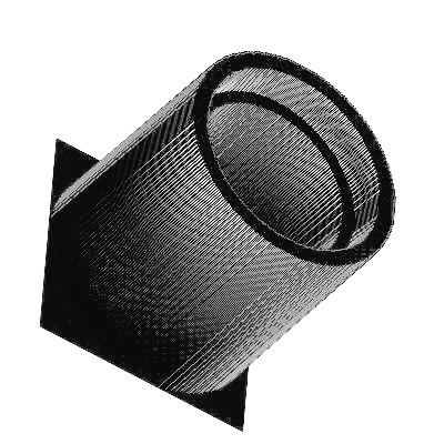
(a) quantum dot

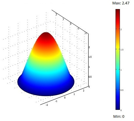
(b) wave function

Figure 1: Wave function and its corresponding quantum dot

Take $\Omega$ to be a ball centered at the origin with radius $R=2.4$ nm in $\mathbb{R}^{2}$. Let $q_{0}(x)$ be a characteristic function (step function) equals $2.13$ eV in a subset of $\Omega$ with area $3.85$ $\mathrm{nm}^{2}$ and is zero elsewhere. Similarly, $p_{0}(x)$ is a characteristic function equals $0.27$ eV in a subset of $\Omega$ with area $2$ $\mathrm{nm}^{2}$ and is zero elsewhere. Assume the particle’s mass is $m=7.81638\times 10^{-32}$ kg, then we have $\gamma=\hbar^{2}/2m=7.114043325\times 10^{-38}\;\mathrm{(J.s)^{2}/kg}$. Recall from (3.2) that $\psi$ is the normalized eigenfunction corresponding to the principal eigenvalue of the Laplacian with Dirichlet’s boundary condition. It is well known that when $\Omega$ is a ball centered at the origin, $\psi=\psi(r)$ is a radial function and in our case can be calculated as follows:

$$\psi(r)=4.528173484\times 10^{8}J_{0}(1.002010649\times 10^{9}r),$$

where $J_{0}$ is the Bessel function of the first kind of order zero [3]. Now, by a simple calculation, it can be verified that $p_{0}$ and $q_{0}$ satisfy conditions (3.1) and (3.2). Applying theorems 3.6 and 4.12 we can deduce that optimal solution of problem (1.2) is the first eigenvalue of (1.1) corresponding to ${p_{0}}_{*}$ and ${q_{0}}_{*}$. In other words, the best potential function is $V={q_{0}}_{*}+2\widehat{\lambda}{p_{0}}_{*}$. Recall that ${p_{0}}_{*}$ and ${q_{0}}_{*}$ are the Schwarz increasing rearrangements of $p_{0}$ and $q_{0}$ respectively. This means that they are two radial characteristic functions with two circular annular regions as their supports. Relation (2.1) leads us to the fact that ${q_{0}}_{*}$ is a step function with the height equals the height of $q_{0}$ in an annulus with outer radius $R$ and inner radius $2.13$ nm and ${p_{0}}_{*}$ is a step function with the height equals the height of $p_{0}$ in an annulus with outer radius $R$ and smaller radius $2.26$ nm. Denote by $h_{p}$ and $h_{q}$ the heights of ${p_{0}}_{*}$ and ${q_{0}}_{*}$ respectively. Then, the radial potential $V={q_{0}}_{*}+2\widehat{\lambda}{p_{0}}_{*}$ is

$$V(r)=\left\{\begin{array}[]{ll}0\quad\;\;\;\;\quad\quad\quad 0<r\leq r_{1},\\ h_{q}\quad\quad\quad\quad\;\;\;r_{1}<r\leq r_{2},\\ h_{q}+2\widehat{\lambda}h_{p}\quad\quad r_{2}<r\leq R,\end{array}\right.$$

where $r_{1}=2.13$ $\mathrm{nm}$, $r_{2}=2.26$ $\mathrm{nm}$ and $R=2.4$ $\mathrm{nm}$. Using this potential, one can construct a three dimensional nanostructure on $\Omega$ which is made of two concentric cylinder nested within each other. These cylinders have heights $h_{q}$ and $h_{q}+2\widehat{\lambda}h_{p}$. When the free carrier is trapped within this structure, the structure can be considered as a quantum dot [1]. The optimal quantum dot is shown in figure 1a schematically.

Inserting ${p_{0}}_{*}$ and ${q_{0}}_{*}$ into (1.1), one can determine the optimal ground state energy employing the standard finite element Galerkin method which yields $\widehat{\lambda}^{2}=0.45$ $(\mathrm{eV})^{2}$ for this typical example. The wave function corresponding to the minimum ground state energy is illustrated in schematic figure 1b.

We can see that $\lambda^{2}$ is less than potential $V$ when $r_{1}\leq r\leq R$. This means that in our quantum dot the energy is confined.

Acknowledgement. The authors would like to express their deep gratitude to anonymous referees for helpful comments and useful suggestions. We would like to acknowledge Professor Heinrich Voss for his thorough reading of the manuscript that help us to improve the presentation of the paper.

6 References

References

• [1] Y. Masumoto, T. Takagahara, Semiconductor quantum dots: physics, spectroscopy and applications series: nanoscience and technology, Springer-Verlag, Berlin, 2002.
• [2] M. Jaulent, C. Jean, The inverse $s$-wave scattering problem for a class of potentials depending on energy, Commun. math. Phys. 28 (1972) 177–220.
• [3] A. Henrot, Extremum problems for eigenvalues of elliptic operators, BirkhΓ€user-Verlag, Basel, 2006.
• [4] F. Cuccu, B. Emamizadeh, G. Porru, Optimization of the first eigenvalue in problems involving the p-Laplacian, Proc. Amer. Math. Soc. 137 (2009) 1677–1687.
• [5] F. Cuccu, G. Porru, S. Sakaguchi Optimization problems on general classes of rearrangements, Nonlinear Anal. 74 (2011) 5554–5565.
• [6] A. Derlet, J.-p. Gossez, P. TakÑč, Minimization of eigenvalues for a quasilinear elliptic Nuemann problem with indefinite wieght, J. Math. Anal. Appl. 371 (2010) 69–79.
• [7] F. Bahrami, B. Emamizadeh, A. Mohammadi, Existence of an extremal ground state energy of a nanostructured quantum dot, Nonlinear Anal. 74 (2011) 6287–6294.
• [8] F.N. Wang, Z.-H. Wei, T.-M. Hwang, W. Wang, A parallel additive Schwarz preconditioned Jacobi-Davidson algorithm for polynomial eigenvalue problems in quantum dot simulation, J. Comput. Phys. 229 (2010) 2932–2947.
• [9] Y. Li, O. Voskoboynikov, C. P. Lee, S. M. Sze, Energy and coordinate dependent effective mass and confined electron states in quantum dots, Solid State Commun. 120 (2001) 79–83.
• [10] O. Voskoboynikov, Y. Li, H. -M. Lu, C.-F. Shih, C.P. Lee, Energy states and magnetization in nanoscale quantum rings, Phys Rev B. 66 (2002) 155306-1–155306-6.
• [11] G.R. Burton, Variational problems on classes of rearrangements and multiple configurations for steady vortices, Ann. Inst. H. Poincar . Anal. Non Lin aire 6. 4 (1989), 295–319.
• [12] A. Alvino, G. Trombetti,P. -L. Lions, On optimization problems with prescribed rearrangements, Nonlinear Anal. 13 (1989) 185–220.
• [13] E. Lieb, M. Loss, Analysis, second edt, American Mathematical Society, Providence, Rhode Island, 2001.
• [14] H. Voss, B. Werner, A minimax principle for nonlinear eigenvalue problems with applications to nonoverdamped systems, Math. Meth. Appl. Sci. 4 (1982) 415 -424.
• [15] H. Voss , A minimax principle for nonlinear eigenvalue problems with applications to a rational spectral problem in fluid-solid vibration, Appl. Math. 48 (2003) 607–622.
• [16] R. Turner , Some variational principles for a nonlinear eigenvalue problem, J. Math. Anal. Appl. 17 (1967) 151–160.
• [17] D. Gilbarg, N.S. Trudinger, Elliptic partial differential equations of second order, second edt, Springer-Verlag, New York, 1998.
• [18] S. Chanillo, D. Grieser, M. Imai, K. Kurata, I. Ohnishi, Symmetry breaking and other phenomena in the optimization of eigenvalues for composite membranes, Commun. Math. Phys. 214 (2000) 315–337.
• [19] A. Mohammadi, F. Bahrami, H. Mohammadpour, Shape dependent energy optimization in quantum dots, Appl. Math. Lett. 25 (2012) 1240–1244.
• [20] G.H. Hardy, J.E. Littlewood, G. PΓ³lya, Inequalities, Cambridge University Press, Cambridge, 1988.
• [21] J.E. Brothers, W.P. Ziemer, Minimal rearrangements of Sobolev functions, J. Reine Angew. Math. 384 (1988) 153–179.
• [22] L. Bers, F. John, M. Schechter, Partial differential equations, Lectures in applied mathematics, vol III, American Mathematical Society Providence, Rhode Island, 1964.
• [23] H. Federer, Geometric measure theory , Springer-Verlag, Berlin, 1969 .
• [24] M.A. Reed, Quantum dots, Sci. Am. 268 (1993) 118–123.