Mixed-valence correlations in charge-transferring atom-surface collisions

Abstract

Motivated by experimental evidence for a mixed-valence state to occur in the neutralization of strontium ions on gold surfaces we analyze this type of charge-transferring atom-surface collision from a many-body theoretical point of view using quantum-kinetic equations together with a pseudo-particle representation for the electronic configurations of the atomic projectile. Particular attention is paid to the temperature dependence of the neutralization probability which–experimentally–seems to signal mixed-valence-type correlations affecting the charge-transfer between the gold surface and the strontium projectile. We also investigate the neutralization of magnesium ions on a gold surface which shows no evidence for a mixed-valence state. Whereas for magnesium excellent agreement between theory and experiment could be obtained, for strontium we could not reproduce the experimental data. Our results indicate mixed-valence correlations to be in principle present, but for the model mimicking most closely the experimental situation they are not strong enough to affect the neutralization process quantitatively.

I Introduction

Charge-exchange between an atomic projectile and a surface plays a central role in surface science. Winter and Burgdörfer (2007); Rabalais (1994); Los and Geerlings (1990); Brako and Newns (1989); Modinos (1987); Yoshimori and Makoshi (1986) Many surface diagnostics, for instance, secondary ion mass spectrometry Czanderna and Hercules (1991) or meta-stable atom de-excitation spectroscopy Harada et al. (1997) utilize surface-based charge-transfer processes. The same holds for plasma science. Surface-based production of negative hydrogen ions, for instance, is currently considered as a pre-stage process in neutral gas heating of fusion plasmas. Kraus et al. (2008) The operation modii of low-temperature gas discharges Lieberman and Lichtenberg (2005), which are main work horses in many surface modification and semiconductor industries, depend on secondary electron emission from the plasma walls and thus also on surface-based charge-transfer processes.

Besides of their great technological importance, charge-transferring atom-surface collisions are however also of fundamental interest. This type of collision couples a local quantum system with a finite number of discrete states–the projectile–to a large reservoir with a continuum of states–the target. Irrespective of the coupling between the two, either due to tunneling or due to Auger-type Coulomb interaction, charge-transferring atom-surface collisions are thus perfect realizations of time-dependent quantum impurity systems. Shao et al. (1996); Merino and Marston (1998) By a judicious choice of the projectile-target combination as well as the collision parameters Kondo-type features Hewson (1993) are thus expected as in any other quantum impurity system. Grabert and Devoret (1992); Wingreen and Meir (1994); Aguado and Langreth (2003); Ternes et al. (2009)

Indeed a recent experiment by He and Yarmoff He and Yarmoff (2010, 2011) provides strong evidence for electron correlations affecting the neutralization of positively charged strontium ions on gold surfaces. The fingerprint of correlations could be the experimentally found negative temperature dependence of the neutralization probability. It may arise Shao et al. (1996); Merino and Marston (1998) from thermally excited conduction band holes occupying the strongly renormalized $5s^{1}$ configuration of the projectile which effectively stabilizes the impinging ion and reduces thereby the neutralization probability. The purpose of the present work is to analyze the He-Yarmoff experiment He and Yarmoff (2010, 2011) from a genuine many-body theoretical point of view, following the seminal work of Nordlander and coworkers Langreth and Nordlander (1991); Nordlander et al. (1993); Shao et al. (1994a, b, 1996) as well as Merino and Marston Merino and Marston (1998) and to provide theoretical support for the interpretation of the experiment in terms of a mixed-valence scenario.

We couch–as usual–the theoretical description of the charge-transferring atom-surface collision in a time-dependent Anderson impurity model. Los and Geerlings (1990); Brako and Newns (1989); Modinos (1987); Yoshimori and Makoshi (1986); Kasai and Okiji (1987); Nakanishi et al. (1988); Romero et al. (2009); Bajales et al. (2007); Goldberg et al. (2005); Onufriev and Marston (1996); Marston et al. (1993) The parameters of the model are critical. To be as realistic as possible without performing an expensive ab-initio analysis of the ion-surface interaction we employ for the calculation of the model parameters Gadzuk’s semi-empirical approach Gadzuk (1967a, b) based on image charges and Hartree-Fock wave functions for the projectile states. Clementi and Roetti (1974) The time-dependent Anderson model, written in terms of pseudo-operators Coleman (1984); Kotliar and Ruckenstein (1986) for the projectile states, is then subjected to a full quantum-kinetic analysis using contour-ordered Green functions Kadanoff and Baym (1962); Keldysh (1965) and a non-crossing approximation for the hybridization self-energies as originally proposed by Nordlander and coworkers. Langreth and Nordlander (1991); Nordlander et al. (1993); Shao et al. (1994a, b, 1996)

We apply the formalism to analyze, respectively, the neutralization of a strontium and a magnesium ion on a gold surface. For the Mg:Au system, which shows no evidence for mixed-valence correlations affecting the charge-transfer between the surface and the projectile, we find excellent agreement between theory and experiment. For the Sr:Au system, in contrast, we could reproduce only the correct order of magnitude of the neutralization probability. Its temperature dependence could not be reproduced. Our modeling shows however that a mixed-valence scenario could in principle be at work. For the material parameters best suited for the description of the Sr:Au system they are however not strong enough to affect the neutralization probability also quantitatively.

The outline of our presentation is as follows. In the next section we describe the time-dependent Anderson model explaining in particular how we obtained the parameters characterizing it. Section III concerns the quantum kinetics and presents the set of coupled two-time integro-differential equations which have to be solved for determining the probabilities with which the various charge states of the projectile occur. They form the basis for the analysis of the temperature dependence of the neutralization probability. Numerical results for a strontium as well as a magnesium ion hitting a gold surface are presented, discussed, and compared to experimental data in Sect. IV. Concluding remarks are given in Sect. V.

II Model

When an atomic projectile approaches a surface its energy levels shift and broaden due to direct and exchange Coulomb interactions with the surface. Since the target and the projectile are composite objects the calculation of these shifts and broadenings from first principles is a complicated problem. Nordlander and Tully (1990) We follow therefore Gadzuk’s semi-empirical approach. Gadzuk (1967a, b) From our previous work on secondary electron emission due to de-excitation of meta-stable nitrogen molecules on metal Marbach et al. (2011) and dielectric Marbach et al. (2012a, b) surfaces we expect the approach to give reasonable estimates for the level widths as well as the level positions for distances from the surface larger than a few Bohr radii. In addition, the approach has a clear physical picture behind it and is thus intuitively very appealing.

The essence of the model is illustrated in Fig. 1. It shows for the particular case of a strontium ion hitting a gold surface the energy levels of the projectile closest to the Fermi energy of the target. Quite generally, for alkaline-earth (AE) ions the first and the second ionization levels are most important. Identifying the positive ion (${\rm AE}^{+}$) with a singly occupied impurity and the neutral atom (${\rm AE}^{0}$) with a doubly occupied impurity, the projectile can be modelled as a non-degenerate, asymmetric Anderson model with on-site energies

$$\varepsilon_{U}(z) =-I_{1}+\frac{e^{2}}{4|z-z_{i}|}~{},$$ (1)

$$\varepsilon_{0}(z) =-I_{2}+\frac{3e^{2}}{4|z-z_{i}|}~{},$$ (2)

where $I_{1}>0$ and $I_{2}>0$ are, respectively, the first and second ionization energy far away from the surface while $z_{i}$ is the distance of the metal’s image plane from its crystallographic ending at $z=0$. The on-site Coulomb repulsion $U(z)$ would be the difference of the two energies. Table 1 summarizes the material parameters required for the modeling of the neutralization of strontium and magnesium ions on a gold surface.

	$I_{1}$[eV]	$Z_{1}$	$I_{2}$[eV]	$Z_{2}$	$\Phi$[eV]	${\rm E_{F}}$[eV]	$z_{\rm i}$[a.u.]	$m_{e}^{*}/m_{e}$
Sr	5.7	1.65	11.0	2	–	–	–	–
Mg	7.65	1.65	15.04	2	–	–	–	–
Au	–	–	–	–	5.1–5.2	5.53	1.0	1.1

Table 1: Material parameters for magnesium, strontium and gold: $I_{1}$ and $I_{2}$ are the first and the second ionization energy, $Z_{1}$ and $Z_{2}$ are the effective charges to be used in the calculation of the hybridization matrix element (viz: Eq. (9)), $\Phi$ is the work function, ${\rm E_{F}}$ the Fermi energy, $z_{i}$ the position of the image plane in front of the surface, and $m_{e}^{*}$ is the effective mass of an electron.

The $z-$dependent shifts of the ionization levels can be obtained as the energy gain of a virtual process moving the configuration under consideration from the actual position $z$ to $z=\infty$, reducing its electron occupancy by one, and then moving it back to position $z$, taking into account in both moves–if present–image interactions due to the charge state of the final and initial configurations with the metal. Newns et al. (1983) For the upper level, $\varepsilon_{U}$, that is, the $5s^{2}$ configuration the cycle is ${\rm AE}\rightarrow{\rm AE}^{+}+e^{-}\rightarrow{\rm AE}^{+}$, whereas for the lower level, $\varepsilon_{0}$, that is, the $5s^{1}$ configuration the cycle is ${\rm AE}^{+}\rightarrow{\rm AE}^{2+}+e^{-}\rightarrow{\rm AE}^{2+}$.

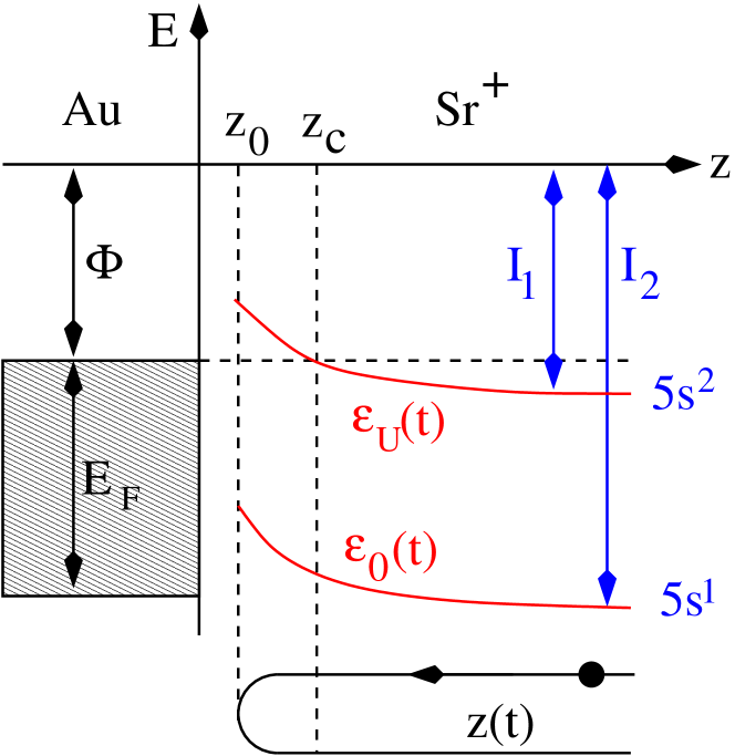
Figure 1: Illustration of the time-dependent quantum impurity model used for the description of the charge-transferring scattering of a ${\rm Sr}^{+}$ ion on a gold surface. The two ionization energies, $\varepsilon_{U}(t)$ and $\varepsilon_{0}(t)$, standing for the projectiles’ $5s^{2}$ and $5s^{1}$ configuration, respectively, shift due to the image interaction with the surface. Far away from the surface the two energies merge, respectively, with the first $(I_{1})$ and the second ($I_{2}$) ionization energy of a strontium atom. The image interaction also leads to a hybridization of the Sr states with the conduction band states of the surface which is characterized by a step potential at $z=0$ whose depth is the sum of the work function $\Phi>0$ and the Fermi energy ${\rm E_{F}}>0$. For simplicity the broadening is not shown. Indicated however is the trajectory $z(t)$ of the ion. Important points along the trajectory are $z_{0}$, the turning point, and $z_{c}$, the point where the first ionization level crosses the Fermi energy.

To set up the Hamiltonian we also need the wave functions for the projectile states. For the upper level we use the (ns) Hartree-Fock wave function of an ${\rm AE}$ atom while for the lower level we use the (ns) Hartree-Fock wave function of an ${\rm AE}^{+}$ ion. According to Clementi and Roetti Clementi and Roetti (1974) both can be written in the form

$$\psi_{\rm HF}(\vec{r}\,) =Y_{00}(\theta,\phi)\sum_{j=1}^{N}c_{j}N_{j}|\vec{r}\,|^{n_{j}-1}e^{-C_{j}|\vec{r}\,|}~{}$$ (3)

with $c_{j},n_{j},C_{j}$, and $N_{j}$ tabulated parameters and $Y_{00}(\theta,\phi)$ the spherical harmonics with $m=l=0$.

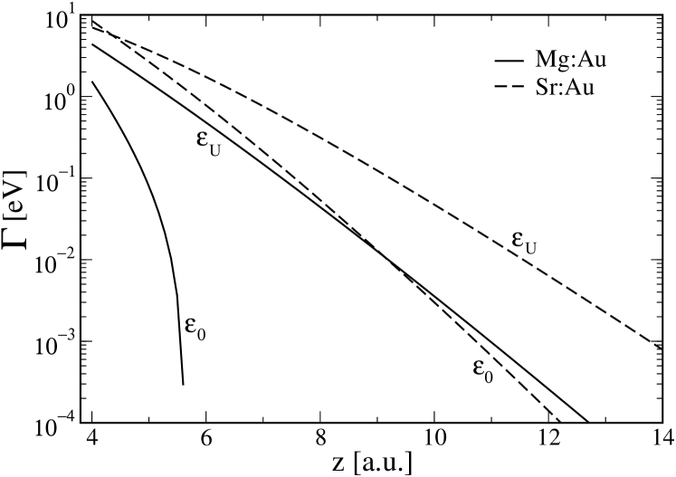
Figure 2: Level widths as obtained from Eq. (10) for the Mg:Au (solid lines) and the Sr:Au (dashed lines) system.

For simplicity we assume the projectile to approach the surface from $z=\infty$ on a perpendicular trajectory,

$$z(t)=z_{0}+v|t|~{},$$ (4)

with the turning point $z_{0}$ reached at time $t=0$ and $v$ the velocity of the projectile. The lateral motion of the projectile is thus ignored. To be consistent with this simple trajectory we also neglect the lateral variation of the potential characterizing the metal surface. The electrons of the metal are thus simply described in terms of a potential step at $z=0$ with depth $-|V_{0}|=\Phi+{\rm E_{F}}$, where $\Phi>0$ is the work function of the metal and ${\rm E_{F}}>0$ is its Fermi energy measured from the bottom of the conduction band (see Table 1), leading to

$$\varepsilon_{\vec{k}} =\frac{\hbar^{2}}{2m^{*}_{e}}\left(k_{x}^{2}+k_{y}^{2}+k_{z}^{2}\right)-\left|V_{0}\right|~{},$$ (5)

$$\psi_{\vec{k}}(\vec{r}\,) =\frac{1}{L\sqrt{L}}\,e^{i\left(k_{x}x+k_{y}y\right)}\Bigl{\{}T_{k_{z}}e^{-\kappa_{k_{z}}z}\Theta(z)$$

$$+\left[e^{ik_{z}z}+R_{k_{z}}e^{-ik_{z}z}\right]\Theta(-z)\Bigr{\}}~{},$$ (6)

for the energies and wave functions of the conduction band electrons; $L$ is the spatial width of the step (drops out in the final expressions) and

$$R_{k_{z}} =\frac{ik_{z}+\kappa_{k_{z}}}{ik_{z}-\kappa_{k_{z}}}~{},$$ (7)

$$T_{k_{z}} =\frac{2ik_{z}}{ik_{z}-\kappa_{k_{z}}}~{},$$ (8)

with $\kappa_{k_{z}}=\sqrt{2m^{*}_{e}(\left|V_{0}\right|-k_{z}^{2})/\hbar^{2}}$ are the reflection and transmission coefficients of the potential step.

While the projectile is on its trajectory its ionization levels hybridize with the conduction band. The matrix element for this process is given by Gadzuk (1967a, b)

$$V_{\vec{k}}(t)=\int_{z>0}\!\!\!\!\!d^{3}r\,\psi_{\vec{k}}^{*}(\vec{r}\,)\frac{Ze^{2}}{|\vec{r}-\vec{r}_{p}(t)|}\psi_{\rm HF}({\vec{r}-\vec{r}_{p}(t)})~{},$$ (9)

where the potential between the two wave functions is the residual Coulomb interaction of the valence electron with the core of the projectile located at $\vec{r}_{p}(t)=z(t)\vec{e}_{z}$. The matrix element can be transformed to a level width

$$\Gamma_{\varepsilon(t)}(t)=2\pi\sum_{\vec{k}}\left|V_{\vec{k}}(t)\right|^{2}\delta(\varepsilon(t)-\varepsilon_{\vec{k}})$$ (10)

which is an important quantity. The charge $Z$ in Eq.(9) is the charge of the nucleus screened by all the electrons of the projectile except of the valence electron under consideration. For the hybridization of the lower level, the second ionization level, $Z=2$ while for the hybridization of the upper level, the first ionization level, $Z=2-s$, where $s=0.35$ is Slater’s shielding constant due to the second electron in the $s$-valence shell. Slater (1930)

In Fig. 2 we show the level widths calculated form Eq. (10) with $\varepsilon(t)$ set, respectively, to $\varepsilon_{U}(t)$ and $\varepsilon_{0}(t)$, for magnesium and strontium using the parameters of Table 1. Most probably we overestimate the widths close to the surface. To what extent, however, only precise calculations of the kind performed for alkaline ions by Nordlander and Tully can show. Nordlander and Tully (1990)

Figure 3: Possible configurations of the AE projectile. Solid and dashed arrows indicate, respectively, spin-reversed states which are energetically degenerate. The quantities $\tilde{n}_{\sigma}$, $n_{d}$, and $n_{e}$ are, respectively, the (pseudo) probabilities with which the ${\rm AE}^{+}$, the ${\rm AE}^{0}$, and the ${\rm AE}^{2+}$ configuration occur.

Using Coleman’s pseudo-particle representation Coleman (1984); Kotliar and Ruckenstein (1986) for the projectile configurations illustrated in Fig. 3, the Hamiltonian describing the interaction of an AE projectile with a metal surface can be written as Shao et al. (1994b)

$$H(t) =\sum_{\sigma}\varepsilon_{0}(t)p_{\sigma}^{\dagger}p_{\sigma}^{\phantom{{\dagger}}}+[\varepsilon_{0}(t)+\varepsilon_{U}(t)]d^{\dagger}d^{\phantom{{\dagger}}}$$

$$+\sum_{\vec{k}\sigma}\varepsilon_{\vec{k}}c_{\vec{k}\sigma}^{\dagger}c_{\vec{k}\sigma}^{\phantom{{\dagger}}}+\sum_{\vec{k}\sigma}\big{[}V_{\vec{k}}(t)c_{\vec{k}\sigma}^{\dagger}e^{\dagger}p_{\sigma}^{\phantom{{\dagger}}}+h.c.\big{]}$$

$$+\sum_{\vec{k}\sigma}\big{[}V_{\vec{k}}(t)c_{\vec{k}\sigma}^{\dagger}d^{\phantom{{\dagger}}}p_{-\sigma}^{\dagger}+h.c.\big{]}$$ (11)

with $e^{\dagger}$, $d^{\dagger}$, and $p_{\sigma}^{\dagger}$ denoting, respectively, the creation operators for an empty (${\rm AE}^{2+}$), a doubly occupied (${\rm AE}^{0}$), and a singly occupied (${\rm AE}^{+}$) projectile. Since the projectile can be only in either one of these configurations, the Hamiltonian has to be constrained by Coleman (1984); Kotliar and Ruckenstein (1986)

$$Q=\sum_{\sigma}p_{\sigma}^{\dagger}p_{\sigma}^{\phantom{{\dagger}}}+d^{\dagger}d^{\phantom{{\dagger}}}+e^{\dagger}e^{\phantom{{\dagger}}}=1~{}.$$ (12)

This completes the description of the model. Combined with measured projectile velocities the model describes the charge-transfer responsible for the neutralization of alkaline-earth ions on noble metal surfaces.

Figure 4: Self-energies in the non-crossing approximation. Straight dashed lines denote bare Green functions for the conduction band electrons. The other lines indicate renormalized Green functions for the singly occupied (p), the empty (e), and the doubly occupied (d) AE projectile. Filled bullets stand for the hybridization matrix element $V_{\vec{k}}(t)$. Diagrams (a) and (b) give, respectively, the self-energies $\Sigma_{0,\sigma}$ and $\Sigma_{U,\sigma}$ for the Green function $P_{\sigma}$. The self-energies $\Pi_{e}$ and $\Pi_{d}$ for the Green functions $E$ and $D$, respectively, are shown in (c) and (d).

III Quantum kinetics

To calculate the neutralization probability for the AE ion hitting the metal surface we follow Nordlander and coworkers Langreth and Nordlander (1991); Nordlander et al. (1993); Shao et al. (1994a, b, 1996) and set up quantum-kinetic equations for contour-ordered Green functions Kadanoff and Baym (1962); Keldysh (1965) describing the empty, singly, and doubly occupied projectile. We denote these functions, respectively, by $E(t,t^{\prime})$, $P_{\sigma}(t,t^{\prime})$, and $D(t,t^{\prime})$ and write their analytic pieces in the form

$$H^{\rm R}(t,t^{\prime}) =-i\Theta(t-t^{\prime})\exp[-i\!\int_{t^{\prime}}^{t}\!\!d\bar{t}\varepsilon(\bar{t})]\bar{H}^{\rm R}(t,t^{\prime})~{},$$ (13)

$$H^{\gtrless}(t,t^{\prime}) =\exp[-i\!\int_{t^{\prime}}^{t}\!\!d\bar{t}\varepsilon(\bar{t})]\bar{H}^{\gtrless}(t,t^{\prime})~{},$$ (14)

where $H(t,t^{\prime})$ can be any of the three Green functions and $\varepsilon(t)$ is, depending on the Green function, either identically $0$, $\varepsilon_{0}(t)$, or $\varepsilon_{0}(t)+\epsilon_{U}(t)$.

Using this notation and calculating the self-energies $\Pi_{e}$, $\Sigma_{0,\sigma}$, $\Sigma_{U,\sigma}$, and $\Pi_{d}$ in the non-crossing approximation diagrammatically shown in Fig. 4 leads after application of the Langreth-Wilkins rules Langreth and Wilkins (1972) and the projection to the $Q=1$ subspace Langreth and Nordlander (1991); Aguado and Langreth (2003) to Shao et al. (1994a, b)

$$\frac{\partial}{\partial t}\bar{E}^{\rm R}(t,t^{\prime}) =-\sum_{\sigma}\int_{t^{\prime}}^{t}\!\!d\bar{t}\bar{K}_{\varepsilon_{0}}^{<}(\bar{t},t)\bar{P}_{\sigma}^{\rm R}(t,\bar{t})\bar{E}^{\rm R}(\bar{t},t^{\prime})~{},$$ (15)

$$\frac{\partial}{\partial t}\bar{P}_{\sigma}^{\rm R}(t,t^{\prime}) =-\int_{t^{\prime}}^{t}\!\!d\bar{t}\bar{K}_{\varepsilon_{0}}^{>}(t,\bar{t})\bar{E}^{\rm R}(t,\bar{t})\bar{P}_{\sigma}^{\rm R}(\bar{t},t^{\prime})$$

$$~{}~{}~{}-\int_{t^{\prime}}^{t}\!\!d\bar{t}\bar{K}_{\varepsilon_{U}}^{<}(\bar{t},t)\bar{D}^{\rm R}(t,\bar{t})\bar{P}_{\sigma}^{\rm R}(\bar{t},t^{\prime})~{},$$ (16)

$$\frac{\partial}{\partial t}\bar{D}^{\rm R}(t,t^{\prime}) =-\sum_{\sigma}\int_{t^{\prime}}^{t}\!\!d\bar{t}\bar{K}_{\varepsilon_{U}}^{>}(t,\bar{t})\bar{P}_{-\sigma}^{\rm R}(t,\bar{t})\bar{D}^{\rm R}(\bar{t},t^{\prime})~{},$$ (17)

and

$$\frac{\partial}{\partial t}\bar{E}^{<}(t,t^{\prime}) =\sum_{\sigma}\int^{t^{\prime}}_{-\infty}\!\!d\bar{t}\bar{K}_{\varepsilon_{0}}^{>}(\bar{t},t)\bar{P}_{\sigma}^{<}(t,\bar{t})[\bar{E}^{\rm R}(t^{\prime},\bar{t})]^{*}-\sum_{\sigma}\int^{t}_{-\infty}\!\!d\bar{t}\bar{K}_{\varepsilon_{0}}^{<}(\bar{t},t)\bar{P}_{\sigma}^{\rm R}(t,\bar{t})\bar{E}^{<}(\bar{t},t^{\prime})~{},$$ (18)

$$\frac{\partial}{\partial t}\bar{P}_{\sigma}^{<}(t,t^{\prime}) =\int^{t^{\prime}}_{-\infty}\!\!d\bar{t}\bar{K}_{\varepsilon_{0}}^{<}(t,\bar{t})\bar{E}^{<}(t,\bar{t})[\bar{P}_{\sigma}^{\rm R}(t^{\prime},\bar{t})]^{*}+\int^{t^{\prime}}_{-\infty}\!\!d\bar{t}\bar{K}_{\varepsilon_{U}}^{>}(\bar{t},t)\bar{D}^{<}(t,\bar{t})[\bar{P}_{\sigma}^{\rm R}(t^{\prime},\bar{t})]^{*}$$

$$-\int^{t}_{-\infty}\!\!d\bar{t}\bar{K}_{\varepsilon_{0}}^{>}(t,\bar{t})\bar{E}^{\rm R}(t,\bar{t})\bar{P}_{\sigma}^{<}(\bar{t},t^{\prime})-\int^{t}_{-\infty}\!\!d\bar{t}\bar{K}_{\varepsilon_{U}}^{<}(\bar{t},t)\bar{D}^{\rm R}(t,\bar{t})\bar{P}_{\sigma}^{<}(\bar{t},t^{\prime})~{},$$ (19)

$$\frac{\partial}{\partial t}\bar{D}^{<}(t,t^{\prime}) =\sum_{\sigma}\int^{t^{\prime}}_{-\infty}\!\!d\bar{t}\bar{K}_{\varepsilon_{U}}^{<}(t,\bar{t})\bar{P}_{-\sigma}^{<}(t,\bar{t})[\bar{D}^{\rm R}(t^{\prime},\bar{t})]^{*}-\sum_{\sigma}\int^{t}_{-\infty}\!\!d\bar{t}\bar{K}_{\varepsilon_{U}}^{>}(t,\bar{t})\bar{P}_{-\sigma}^{\rm R}(t,\bar{t})\bar{D}^{<}(\bar{t},t^{\prime})~{}$$ (20)

with

$$\bar{K}_{\varepsilon}^{\gtrless}(t,t^{\prime})=\sqrt{\Gamma_{\varepsilon(t)}(t)\Gamma_{\varepsilon(t^{\prime})}(t^{\prime})}\bar{f}_{\varepsilon}^{\,\gtrless}(t,t^{\prime})$$ (21)

and

$$\bar{f}_{\varepsilon}^{\,\gtrless}(t,t^{\prime})=\exp[i\!\int_{t^{\prime}}^{t}\!\!d\bar{t}\varepsilon(\bar{t})]f^{\,\gtrless}(t-t^{\prime})~{},$$ (22)

where $f^{<}(t)=1-f^{>}(t)$ is the Fourier transform of the Fermi function $f^{<}(\varepsilon)$ defined by

$$f^{<}(t)=\int\frac{d\varepsilon}{2\pi}f^{<}(\varepsilon)\exp[-i\varepsilon t]~{}.$$ (23)

The function $\bar{K}_{\varepsilon}^{\gtrless}(t,t^{\prime})$, which contains the temperature dependence, entails an approximate momentum summation. From the diagrams shown in Fig. 4 one initially obtains

$$K^{\gtrless}(t,t^{\prime})=\int\!\frac{d\varepsilon}{2\pi}\sqrt{\Gamma_{\varepsilon}(t)\Gamma_{\varepsilon}(t^{\prime})}f^{\gtrless}(\varepsilon)\exp[-i\varepsilon(t-t^{\prime})]$$ (24)

with an energy integration extending over the range of the conduction band and $\Gamma_{\varepsilon}(t)$ given by Eq. (10) with $\varepsilon(t)$ replaced by the integration variable $\varepsilon$. To avoid the numerically costly energy integration Nordlander and coworkers employed two different approximations: In Ref. Shao et al., 1994a they replaced $\Gamma_{\varepsilon}(t)$ by an average over the energy range of the conduction band while in Ref. Shao et al., 1994b they replaced it by $\Gamma_{\varepsilon(t)}(t)$ with $\varepsilon(t)$ set to $\varepsilon_{0}(t)$ or $\varepsilon_{U}(t)$ depending on which state is considered in the hybridization self-energy. Using the latter leads to

$$K_{\varepsilon}^{\gtrless}(t,t^{\prime})\simeq\sqrt{\Gamma_{\varepsilon(t)}(t)\Gamma_{\varepsilon(t^{\prime})}(t^{\prime})}f^{\gtrless}(t-t^{\prime})$$ (25)

and eventually to $\bar{K}_{\varepsilon}^{\gtrless}(t,t^{\prime})$ as given in Eq. (21). The subscript $\varepsilon$ indicates now not an integration variable but the functional dependence on $\varepsilon(t)$. We employ this form but keep in mind that it is an approximation to the non-crossing self-energies.

The instantaneous (pseudo) occurrence probabilities for the projectile configurations ${\rm AE}^{2+}$, ${\rm AE}^{+}$, and ${\rm AE}^{0}$ are then given by

$$n_{e}(t) =\bar{E}^{<}(t,t)~{},$$ (26)

$$\tilde{n}_{\sigma}(t) =\bar{P}^{<}_{\sigma}(t,t)~{},$$ (27)

$$n_{d}(t) =\bar{D}^{<}(t,t)~{},$$ (28)

respectively, where we refer to all of them as (pseudo) occurrence probabilities also strictly speaking $n_{d}$ and $n_{e}$ are true ones and only $\tilde{n}_{\sigma}$ is a pseudo occurrence probability in the sense that the true probability with which the ${\rm AE}^{+}$ configuration occurs is $n_{\sigma}=\tilde{n}_{\sigma}+n_{d}$. Shao et al. (1994b) Sometimes we will also refer to $n_{e}$, $\tilde{n}_{\sigma}$, and $n_{d}$ simply as (pseudo) occupancies. For the AE ion the probability for neutralization at the surface (wall recombination) is the probability for double occupancy after the completion of the trajectory, that is,

$$\alpha_{w}=n_{d}(\infty)~{},$$ (29)

subject to the initial conditions $n_{d}(-\infty)=n_{e}(-\infty)=0$ and $\tilde{n}_{\sigma}(-\infty)=\delta_{\sigma,1/2}$.

We solve the two coupled sets of integro-differential equations (15)–(17) and (18)–(20) on a two-dimensional time grid setting

$$\bar{E}^{\rm R}(t,t)=\bar{P}_{\sigma}^{\rm R}(t,t)=\bar{D}^{\rm R}(t,t)=1$$ (30)

for the retarded Green functions and

$$E^{<}(-\infty,-\infty) =n_{e}(-\infty)=0~{},$$ (31)

$$P_{\sigma}^{<}(-\infty,-\infty) =\tilde{n}_{\sigma}(-\infty)=\delta_{\sigma,1/2}~{},$$ (32)

$$D^{<}(-\infty,-\infty) =n_{d}(-\infty)=0$$ (33)

for the less-than Green functions using basically the same numerical strategy as Shao and coworkers. Shao et al. (1994a, b)

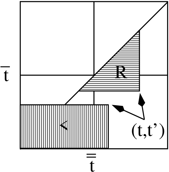
Figure 5: Sketch of the domains in the $(\bar{\bar{t}},\bar{t})$ plane over which Eqs.(15)–(17) and (18)–(20) have to be integrated subject to the boundary conditions (30) and (31)–(33), respectively, in order to determine the retarded and less-than Green functions at $(t,t^{\prime})$. The triangular (rectangular) region denotes the domain required for the calculation of the retarded (less-than) Green functions.

Due to the intertwining of the time integrations the integration domains for the retarded Green functions are triangular whereas for the less-than Green function they are rectangular as shown in Fig. 5. The size of the time-grid as well as the discretization depend on the velocity of the projectile and the maximum distance it has from the surface. For the He-Yarmoff experiment the velocities are on the order of $0.01$ in atomic units. The maximum distance from which the ion starts its journey can be taken to be 20 Bohr radii. At this distance the coupling between the surface and the ion is vanishingly small. We empirically found the algorithm to converge for a $N\times N$ grid with $N=1000-3000$. Since the Green functions are complex the computations are time and memory consuming.

IV Results

We now analyze the He-Yarmoff experiment He and Yarmoff (2010, 2011) quantitatively from a many-body theoretical point of view. For that purpose we combine the model developed in Sect. II with the quantum-kinetics described in Sect. III. Besides the parameters given in Table 1 we also need the velocity of the projectile. In general, the velocity will be different on the in- and outgoing branch of the trajectory. The outgoing branch, however, determines the final charge state of the projectile. We take therefore–for both branches–the normal component of the experimentally measured post-collision velocity. If not noted otherwise all quantities are in atomic units, that is, energies are measured in Hartrees and lengths in Bohr radii.

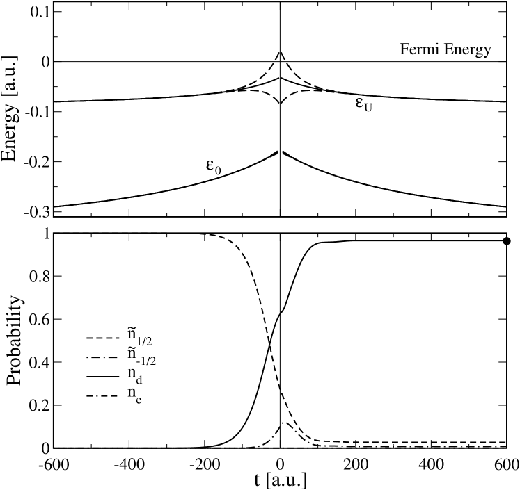
Figure 6: Upper panel: Energy level diagram for the Mg:Au system at $T_{s}=400~{}$K as a function of time. The projectile starts at $t=-600$ and $z=z_{\rm max}=20$ with velocity $v=0.024$, reaches at $t=0$ the turning point $z=z_{0}=5$, and approaches at $t=600$ again $z_{\rm max}$. The ionization levels (solid lines) are broadened according to $\epsilon_{0,U}\pm\Gamma_{0,U}$ (dashed lines) with $\Gamma_{0,U}$ as shown in Fig. 2. Lower Panel: Instantaneous (pseudo) occurrence probabilities along the trajectory for the ${\rm Mg}^{+}$, the ${\rm Mg^{0}}$, and the ${\rm Mg}^{2+}$ configurations. Initially, at time $t=-600$, the projectile is in the ${\rm Mg}^{+}$ configuration. The neutralization probability in this particular case is $\alpha_{w}=n_{d}(600)=0.965$ (solid bullet).

First, we discuss the Mg:Au system. In Fig. 6 we show the time-dependence of the broadened ionization levels, $\varepsilon_{U}$ and $\varepsilon_{0}$, together with the instantaneous (pseudo) occurrence probabilities $\tilde{n}_{\pm 1/2},n_{d}$, and $n_{e}$ for the ${\rm Mg}^{+}$, the ${\rm Mg}^{0}$, and the ${\rm Mg}^{2+}$ configuration, respectively. Negative and positive times denote the in- and outcoming branch of the trajectory. The velocity $v=0.024$ and the surface temperature $T_{s}=400~{}{\rm K}$. Initially, the projectile is in the ${\rm Mg}^{+}$ configuration, that is, the lower level $\varepsilon_{0}$, representing single occupancy, is occupied while the upper level $\varepsilon_{U}$, representing double occupancy, and thus the ${\rm Mg}^{0}$ configuration, is empty. While the projectile is on its way through the trajectory the ionization levels shift and broaden. As a result the occupancies change. The neutralization probability is then the probability for double occupancy at the end of the trajectory.

For the particular case of the Mg:Au system the first ionization level, $\varepsilon_{U}$, that is, the level which has to accept an electron in order to neutralize the ion, is below the Fermi energy of the metal throughout the whole trajectory. The broadening is also rather weak. It only leaks for a very short time span above the Fermi energy. As a result, the magnesium ion can efficiently soak in a second electron while the electron already present due to the initial condition is basically frozen in the second ionization level. The electron captured from the metal has moreover a strong tendency to stay on the projectile. It only has a chance to leave it in the short time span where the instantaneous broadening $\Gamma_{U}(t)$ is larger than $|{\rm E_{F}}-\varepsilon_{U}(t)|$. The neutralization probability is thus expected to be close to unity. Indeed, we find for the situation shown in Fig. 6 $\alpha_{w}=n_{d}(\infty)=0.965$ (solid bullet in Fig. 6).

The temperature dependence of $\alpha_{w}$ is shown in Fig. 7. In accordance with experiment we find $\alpha_{w}$ essentially to be independent of temperature. This is expected because both ionization levels, $\varepsilon_{U}$ and $\varepsilon_{0}$, are below the Fermi energy and their broadening is too small to allow a charge-transfer from the projectile to empty conduction band states of the surface. Notice, the excellent agreement between theory and experiment indicating that the semi-empirical model we developed in Sect. II captures the essential features of the charge-transfer pretty well.

Figure 7: Temperature dependence of the neutralization probability $\alpha_{w}=n_{d}(\infty)$ for a ${\rm Mg}^{+}$ ion hitting with $v=0.024$ a gold surface. The turning point $z_{0}=5$. Also shown are experimental data from Ref. He and Yarmoff, 2011.

After the successful description of the Mg:Au system let us now turn to the Sr:Au system. In Fig. 8 we again plot as a function of time the broadened ionization levels and the (pseudo) occurrence probabilities for the three configurations of the projectile. As it was the case for Mg:Au, the configuration of the projectile, which initially was in the configuration representing single occupancy, changes along the trajectory. The changes are however more subtle.

The reason is the level structure. In contrast to the Mg:Au system, the ionization levels are now closer to the Fermi energy of the surface. The first ionization level $\varepsilon_{U}$ even crosses the Fermi energy with far reaching consequences. The part of the trajectory where $\varepsilon_{U}$ is below the Fermi energy, that is, the region where the neutral atom would be energetically favored, the broadening is very small, indicating negligible charge-transfer from the metal to the ion and hence a stabilization of the ion due to lack of coupling. When the broadening and thus the coupling is large $\varepsilon_{U}$ is above the Fermi level. In this part of the trajectory the ion is energetically stabilized. The first ionization level of strontium can capture an electron from the metal only in the time span where $|{\rm E_{F}}-\varepsilon_{U}(t)|<\Gamma_{U}(t)$. The neutralization probability of a strontium ion should be thus much smaller than the one for a magnesium ion. Indeed we find $\alpha_{w}=n_{d}(\infty)=0.046$ which is much smaller than unity (solid bullet in Fig. 8).

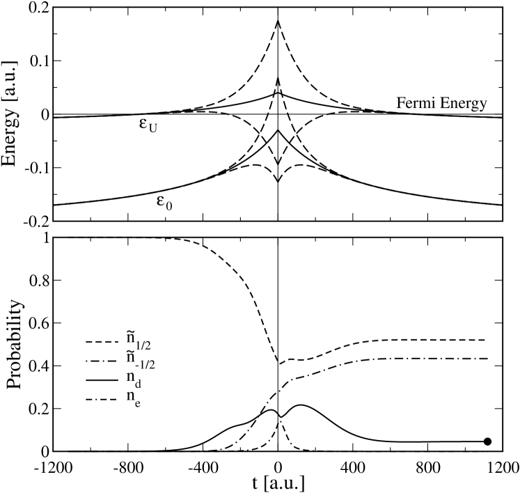
Figure 8: Upper panel: Energy level diagram for the Sr:Au system at $T_{s}=400$ K as a function of time. The projectile starts at $t=-1120$ and $z=z_{\rm max}=20$ with velocity $v=0.0134$, reaches at $t=0$ the turning point $z=z_{0}=5$, and approaches at $t=1120$ again $z=z_{\rm max}$. The levels (solid lines) are broadened according to $\epsilon_{0,U}\pm\Gamma_{0,U}$ (dashed lines) with $\Gamma_{0,U}$ as shown in Fig. 2. Lower Panel: Instantaneous (pseudo) occurrence probabilities along the trajectory for the ${\rm Sr}^{+}$, the ${\rm Sr^{0}}$, and the ${\rm Sr}^{2+}$ configurations. Initially, at time $t=-1120$, the projectile is in the ${\rm Sr}^{+}$ configuration. The neutralization probability in this particular case is $\alpha_{w}=n_{d}(1120)=0.046$ (solid bullet).

Due to the shift and broadening of the first ionization level $\varepsilon_{U}$ it is clear that a strontium ion cannot as efficiently neutralize on a gold surface as a magnesium ion. This sets the scale of $\alpha_{w}$. In addition, and in great contrast to magnesium, the second ionization level $\varepsilon_{0}$ is however also close to the Fermi energy. In those parts of the trajectory for which $|{\rm E_{F}}-\varepsilon_{0}(t)|<\Gamma_{0}(t)$ it can affect the charge-transfer between the metal and the projectile. In fact, taken by itself, it should stabilize the ion and hence decrease the neutralization probability. Merino and Marston (1998) Qualitatively, this can be understood from a density of states argument. From the upper panel of Fig. 8 we can infer that the broadened second ionization level is cut by the Fermi energy in the upper half of its local density of states. Hence, close to the surface holes start to occupy the second ionization level at energies where the local density of states is higher than at the energies where electrons are transferred. Increasing temperature enhances thus the tendency of electron loss from the second ionization level. Without interference from the first ionization level the neutralization probability should thus go down with temperature.

Figure 9: Temperature dependence of the neutralization probability $\alpha_{w}=n_{d}(\infty)$ for a ${\rm Sr}^{+}$ ion hitting with $v=0.0134$ a gold surface. The turning point $z_{0}=5$. Also shown are experimental data from Ref. He and Yarmoff, 2011.

That the second ionization level of Sr comes close to the Fermi energy of Au most probably led He and Yarmoff He and Yarmoff (2010, 2011) to suggest that the neutralization of strontium ions on gold surfaces is dominated by electron correlations. Indeed the experimentally found negative temperature dependence of $\alpha_{w}$ above $T_{s}=600~{}{K}$ seems to support their conclusion. However, the temperature dependence of $\alpha_{w}$ we obtain and which we plot in Fig. 9, does not show this behavior, at least, for the material parameters of Table 1 and the experimentally measured post-collision velocity. The reason for the discrepancy between the measured and the calculated data is unclear. The material parameters seem to be reasonable since the theoretical results have the correct order of magnitude. It could be however that the temperature-induced transfer of holes to the second ionization level is overcompensated by the electron-transfer to the first ionization level. In the region where charge-transfer is strongest the two ionization levels overlap. The absence of energy separation together with the conditional temporal weighting due to the dynamics of the collision process makes it very hard to tell a priori which process will win and manifest itself in the measured neutralization probability.

So far, the discussion of the data left out the possibility of a correlation-induced sharp resonance in the vicinity of the Fermi energy, that is, the key feature of Kondo-type physics. The numerical results seem to suggest that either there is no resonance or it does not affect the neutralization process. However, from the data itself we cannot determine which one is the case. We can thus not decide whether the Sr:Au system is in a correlated regime or not and hence whether an interpretation of the experimental data in terms of a mixed-valence scenario is in principle plausible or has to be dismissed. A rigorous way to decide this would be to calculate the instantaneous spectral functions for the projectile and to look for sharp resonances in the vicinity of the Fermi energy. This is beyond the scope of the present work.

To get at least a qualitative idea about in what regime the strontium projectile might be along its trajectory we plot in Fig. 10, following Merino and Marston, Merino and Marston (1998) Haldane’s scaling invariant, Haldane (1978)

$$\frac{\varepsilon_{0}^{*}}{\Delta_{0}}=\varepsilon_{0}+\frac{\Delta_{0}}{\pi}\log\bigg{(}\frac{U}{\Delta_{0}}\bigg{)}~{},$$ (34)

as a function of time travelled along the outgoing branch of the trajectory. In the perturbative regime which is strictly applicable only far away from the surface $\varepsilon_{0}^{*}$ can be interpreted as the renormalized second ionization level and $\Delta_{0}=\Gamma_{0}/2$. Shao et al. (1994b) For $|\varepsilon_{0}^{*}/\Delta_{0}|<1$ the projectile is likely to be in the mixed-valence regime. Merino and Marston (1998) Since $\varepsilon_{0}^{*}$ comes very close to the Fermi energy holes are expected to transfer in the mixed-valence regime very efficiently to the projectile. In situations where the projectile stays sufficiently long in the mixed-valence regime before $\varepsilon_{0}^{*}$ crosses the Fermi energy double occupancy and hence the neutralization probability should be suppressed with increasing temperature.

As can be seen in Fig. 10 close enough to the surface the strontium projectile is indeed in the mixed-valence regime. For the material parameters given in Table 1 and the experimental value for the projectile velocity the time-span however is rather short. Most probably this is the reason why we do not see any reduction of $\alpha_{w}$ with temperature for the parameters we think to be best suited for the Sr:Au system. Since the experimental data are unambiguous, this indicates perhaps the need for a precise first-principle calculation of the model parameters. Alternative interpretations of the experimental results can however not be ruled out.

Figure 10: Renormalized ($\varepsilon_{0}^{*}$) and bare ($\varepsilon_{0}$) second ionization level measured from the Fermi energy as a function of time traveled along the outgoing branch of the trajectory for the ${\rm Sr}$:Au system with $v=0.0134$ and $T_{s}=400~{}{\rm K}$. Also shown as a function of time is the scaling invariant $\varepsilon_{0}^{*}/\Delta_{0}$. In the region for which $|\varepsilon_{0}^{*}/\Delta_{0}|<1$ the system is likely to be in the mixed-valence region. The material parameters are as given in Table 1 and $v=0.0134$.

V Conclusions

Motivated by claims that the neutralization of strontium ions on gold surfaces is affected by electron correlations we set up a semi-empirical model for charge-transferring collisions between alkaline-earth projectiles and noble metal surfaces. The surface is simply modelled by a step potential while the projectile is modelled by its two highest ionization levels which couple to the surface via Gadzuk’s image-potential-based projectile-surface interaction. To calculate the neutralization probability we employed a pseudo-particle representation of the projectile’s charge states and quantum-kinetic equations for the retarded and less-than Green functions of the projectile as initially suggested by Nordlander, Shao and Langreth. Besides the non-crossing approximation for the self-energies and an approximate momentum summation no further approximations are made. The quantum-kinetic equations are numerically solved on a two-dimensional time-grid using essentially the same strategy as Shao and coworkers.

The absolute values for the neutralization probability we obtain are in good agreement with experimental data, especially for the Mg:Au system, but also for the Sr:Au system, although for the latter we could not reproduce the temperature dependence of the neutralization probability. Our calculations can thus not decide whether the He-Yarmoff experiment can be interpreted in terms of a mixed-valence scenario. From the instantaneous values of Haldane’s scaling invariant we see however that the Sr:Au system could be in the mixed-valence regime. The mechanism for a negative temperature dependence, that is, the possibility of efficiently transferring holes to the second ionization level, is thus in principle present. For the material parameters however most appropriate for Sr:Au the negative temperature dependence arising from this channel seems to be overcompensated by the positive temperature dependence of the electron-transfer to the first ionization level. To proof that He and Yarmoff have indeed seen–for the first time–mixed-valence correlations affecting charge-transfer between an ion and a surface requires therefore further theoretical work.

References

- Winter and Burgdörfer (2007) H.-P. Winter and J. Burgdörfer, eds., Slow heavy-particle induced electron emission from solid surface (Springer-Verlag, Berlin Heidelberg, 2007).
- Rabalais (1994) J. W. Rabalais, ed., Low energy ion-surface interaction (Wiley and Sons, New York, 1994).
- Los and Geerlings (1990) J. Los and J. J. C. Geerlings, Physics Reports 190, 133 (1990).
- Brako and Newns (1989) R. Brako and D. M. Newns, Rep. Prog. Phys. 52, 655 (1989).
- Modinos (1987) A. Modinos, Prog. Surf. Science 26, 19 (1987).
- Yoshimori and Makoshi (1986) A. Yoshimori and K. Makoshi, Prog. Surf. Science 21, 251 (1986).
- Czanderna and Hercules (1991) A. W. Czanderna and D. M. Hercules, Ion spectroscopies for surface analysis (Plenum Press, New York, 1991).
- Harada et al. (1997) Y. Harada, S. Masuda, and H. Ozaki, Chem. Rev. 97, 1897 (1997).
- Kraus et al. (2008) W. Kraus, H.-D. Falter, U. Fantz, P. Franzen, B. Heinemann, P. McNeely, R. Riedl, and E. Speth, Rev. Sci. Instrum. 79, 02C108 (2008).
- Lieberman and Lichtenberg (2005) M. A. Lieberman and A. J. Lichtenberg, Principles of plasma discharges and materials processing (Wiley-Interscience, New York, 2005).
- Shao et al. (1996) H. Shao, D. C. Langreth, and P. Nordlander, Phys. Rev. Lett. 77, 948 (1996).
- Merino and Marston (1998) J. Merino and J. B. Marston, Phys. Rev. B 58, 6982 (1998).
- Hewson (1993) A. C. Hewson, ed., The Kondo problem to heavy fermions (Cambridge University Press, Cambridge, 1993).
- Grabert and Devoret (1992) H. Grabert and M. H. Devoret, eds., Single charge tunneling: Coulomb blockade phenomena in nanostructures (Plenum Press, New York, 1992).
- Wingreen and Meir (1994) N. S. Wingreen and Y. Meir, Phys. Rev. B 49, 11040 (1994).
- Aguado and Langreth (2003) R. Aguado and D. C. Langreth, Phys. Rev. B 67, 245307 (2003).
- Ternes et al. (2009) M. Ternes, A. J. Heinrich, and W.-D. Schneider, J. Phys. C 21, 1 (2009).
- He and Yarmoff (2010) X. He and J. A. Yarmoff, Phys. Rev. Lett. 105, 176806 (2010).
- He and Yarmoff (2011) X. He and J. A. Yarmoff, Nucl. Instrum. Meth. Phys. Res. B 269, 1195 (2011).
- Langreth and Nordlander (1991) D. C. Langreth and P. Nordlander, Phys. Rev. B 43, 2541 (1991).
- Nordlander et al. (1993) P. Nordlander, H. Shao, and D. C. Langreth, Nucl. Instrum. Meth. Phys. Res. B 78, 11 (1993).
- Shao et al. (1994a) H. Shao, D. C. Langreth, and P. Nordlander, Phys. Rev. B 49, 13929 (1994a).
- Shao et al. (1994b) H. Shao, D. C. Langreth, and P. Nordlander, in Low energy ion-surface interaction, edited by J. W. Rabalais (Wiley and Sons, New York, 1994b), p. 117.
- Kasai and Okiji (1987) H. Kasai and A. Okiji, Surface science 183, 147 (1987).
- Nakanishi et al. (1988) H. Nakanishi, H. Kasai, and A. Okiji, Surface science 197, 515 (1988).
- Romero et al. (2009) M. A. Romero, F. Flores, and E. C. Goldberg, Phys. Rev. B 80, 235427 (2009).
- Bajales et al. (2007) N. Bajales, J. Ferrón, and E. C. Goldberg, Phys. Rev. B 76, 245431 (2007).
- Goldberg et al. (2005) E. C. Goldberg, F. Flores, and R. C. Monreal, Phys. Rev. B 71, 035112 (2005).
- Onufriev and Marston (1996) A. V. Onufriev and J. B. Marston, Phys. Rev. B 53, 13340 (1996).
- Marston et al. (1993) J. B. Marston, D. R. Andersson, E. R. Behringer, B. H. Cooper, C. A. DiRubio, G. A. Kimmel, and C. Richardson, Phys. Rev. B 48, 7809 (1993).
- Gadzuk (1967a) J. W. Gadzuk, Surface Science 6, 133 (1967a).
- Gadzuk (1967b) J. W. Gadzuk, Surface Science 6, 159 (1967b).
- Clementi and Roetti (1974) E. Clementi and C. Roetti, Atomic. Data Nucl. Data Tables 14, 177 (1974).
- Coleman (1984) P. Coleman, Phys. Rev. B 29, 3035 (1984).
- Kotliar and Ruckenstein (1986) G. Kotliar and A. E. Ruckenstein, Phys. Rev. Lett. 57, 1362 (1986).
- Kadanoff and Baym (1962) L. P. Kadanoff and G. Baym, Quantum Statistical Mechanics (Benjamin, New York, 1962).
- Keldysh (1965) L. V. Keldysh, Sov. Phys. JETP 20, 1018 (1965).
- Nordlander and Tully (1990) P. Nordlander and J. C. Tully, Phys. Rev. B 42, 5564 (1990).
- Marbach et al. (2011) J. Marbach, F. X. Bronold, and H. Fehske, Phys. Rev. B 84, 085443 (2011).
- Marbach et al. (2012a) J. Marbach, F. X. Bronold, and H. Fehske, Eur. Phys. J. D 66, 106 (2012a).
- Marbach et al. (2012b) J. Marbach, F. X. Bronold, and H. Fehske, Phys. Rev. B 86, 115417 (2012b).
- Newns et al. (1983) D. M. Newns, K. Makoshi, R. Brako, and J. N. M. van Wunnik, Physica Scripta T6, 5 (1983).
- Slater (1930) J. C. Slater, Physical Review 36, 57 (1930).
- Langreth and Wilkins (1972) D. C. Langreth and J. W. Wilkins, Phys. Rev. B 6, 3189 (1972).
- Haldane (1978) F. D. M. Haldane, Phys. Rev. Lett. 40, 416 (1978).