Mirages in galaxy scaling relations

Abstract

We analyzed several basic correlations between structural parameters of galaxies. The data were taken from various samples in different passbands which are available in the literature. We discuss disc scaling relations as well as some debatable issues concerning the so-called Photometric Plane for bulges and elliptical galaxies in different forms and various versions of the famous Kormendy relation.

We show that some of the correlations under discussion are artificial (self-correlations), while others truly reveal some new essential details of the structural properties of galaxies. Our main results are as follows:

(1) At present, we can not conclude that faint stellar discs are, on average, more thin than discs in high surface brightness galaxies. The “central surface brightness – thickness” correlation appears only as a consequence of the transparent exponential disc model to describe real galaxy discs.

(2) The Photometric Plane appears to have no independent physical sense. Various forms of this plane are merely sophisticated versions of the Kormendy relation or of the self-relation involving the central surface brightness of a bulge/elliptical galaxy and the Sérsic index $n$.

(3) The Kormendy relation is a physical correlation presumably reflecting the difference in the origin of bright and faint ellipticals and bulges.

We present arguments that involve creating artificial samples to prove our main idea.

1 Introduction

Global characteristics of galaxies (luminosity, size, rotational velocity, velocity dispersion, etc.) are not distributed randomly, but form a set of well-defined scaling relations. These relations are of great importance since they provide invaluable constraints on the formation scenarios and evolutionary processes of galaxies. The success of any particular theory will be judged by its ability to reproduce the slope, scatter, and zero-point of known scaling relations.

One of the most firmly established empirical scaling relations of elliptical galaxies is the Fundamental Plane (FP) which represents a tight correlation between the surface brightness, the size, and the velocity dispersion of a galaxy (Djorgovski & Davis, 1987; Dressler et al., 1987). Two different projections of the FP are also well-known: the Kormendy and the Faber–Jackson relations (Kormendy, 1977a, b; Faber & Jackson, 1976).

Spiral galaxies are more complex since they consist of a disc, a bulge, and some other components like, for instance, a bar and a ring. The multi-component structure of spiral galaxies results in a variety of scaling relations involving parameters associated with a disc, a bulge, and a galaxy as a whole. The most famous relation is, of course, the Tully–Fisher law (Tully & Fisher, 1977) which links galactic total luminosity and rotation velocity (usually taken as the maximum of the rotation curve well away from the center).

A tight scaling relation may also exist between the photometric and kinematic characteristics of the discs alone. For instance, Karachentsev (1989), Moriondo, Giovanelli & Haynes (1999), and others have discussed a three-dimensional plane involving the disc scalelength $h$, the maximal rotational velocity $v_{\mathrm{m}}$, and the deprojected central surface brightness $S_{\mathrm{0,d}}$. This plane is analogous to the FP of elliptical galaxies.

Edge-on spiral galaxies provide a possibility to analyze the vertical surface brightness distribution and, therefore, add a new parameter to scaling relations — the vertical scaleheight, typically, $h_{z}$ for the exponential vertical surface brightness distribution (Wainscoat, Freeman & Hyland, 1989) or $z_{0}$ for the ‘isothermal’ law (Spitzer, 1942; van der Kruit & Searle, 1981a, b, 1982a, 1982b). A significant correlation between the central surface brightness of a stellar disc reduced to the face-on orientation $S_{\mathrm{0,d}}$ and the ratio $h/z_{0}$ was found: the thinner the galaxy, the fainter the central surface brightness (Bizyaev & Mitronova, 2002; Bizyaev & Kajsin, 2004; Bizyaev & Mitronova, 2009).

Bulges of spiral galaxies also show several empirical relations. For instance, they follow a relation similar to the FP for elliptical galaxies (e.g. , 2002). Khosroshahi et al. (2000a) and (2000b) found a tight correlation between the Sérsic index $n$, the central surface brightness $\mu_{\mathrm{0,b}}$, and the effective radius of the bulge $r_{\mathrm{e,b}}$. They called this relationship the photometric plane (PhP). The PhP projection — the correlation between the central surface brightness of a bulge $\mu_{\mathrm{0,b}}$ and its Sérsic index $n$ — is known as well (e.g. , 2000b; Möllenhoff & Heidt, 2001; Aguerri et al., 2004; Ravikumar et al., 2006; Barway et al., 2009). Also, there exist mutual correlations between the structural parameters of discs and bulges (e.g. , 2010, MSR10 hereafter, and references therein).

In this paper, we critically examine several important scaling relations of spiral and elliptical galaxies focusing on spirals, their discs and bulges. Our main conclusion is that some of these empirical relations (the deprojected central surface brightness – the relative thickness of the disc, the central surface brightness of the bulge — the Sérsic index, the PhP for ellipticals and bulges of spirals) are not physical, and they merely reflect the structure of fitting formulas. In other words, these scaling relations are spurious self-correlations, or mirages of the approximation procedures. Such spurious self-correlations arise when two parameters, for example, $A$ and $B$ that are used in a linear regression analysis, have a common term: $A=f(x)$ and $B=f(x)+g(y)$, where $x$ and $y$ are random, uncorrelated variables. In this case, any correlation found between $A$ and $B$ has no physical meaning and is entirely due to the self-correlation associated with the shared variable $x$. Thus, self-correlations link a measured parameter $A$ with an expression $B$ including the same parameter. Examples are presented to show that under certain conditions perfect (but entirely spurious) correlation is obtained between two such parameters formed from random numbers.

On the other hand, we show that the curvature of the Kormendy relation is real and can not be explained in terms of other linear relations unifying faint and bright galaxies as well as faint and bright bulges (Graham & Guzmán, 2003; Graham, 2011, 2013a).

This paper is organized as follows. In Section 2, we describe the samples analyzed in this paper. We briefly discuss the methods of deriving photometric parameters of bulges and discs. In Section 3, we discuss one well-known scaling relation for edge-on discs (between the central surface brightness of a stellar disc and the relative thickness) and show that it is a self-correlation. In Section 4, we demonstrate that the Photometric Plane for bulges, and ellipticals, and its various forms are merely the self-relation involving the central surface brightness of a bulge/elliptical and the Sérsic index $n$ or sophisticated versions of the Kormendy relation. In Section 5, we present arguments in favor of the reality of the Kormendy relation which do reveal important features of the galaxy structure. In Section 6, we summarize our main conclusions.

2 The samples

We consider some of the most well-known samples with published decomposition results. The samples of edge-on galaxies are provided in Table 1. Other selected samples of galaxies are listed in Table 2. These samples comprise objects of different morphological types as well as are given in different photometric bands. Some samples are quite enormous (Simard et al., 2011) or huge (e.g., Allen et al., 2006 and Gadotti, 2009, hereafter G09) whereas others consist of only tens objects. We do not consider spheroidal galaxies and “core” elliptical galaxies since they are out of the scope of this article.

Table 1: List of analyzed samples of edge-on galaxies with derived structural parameters of discs.

Reference	Number of galaxies	Band	Morphological types
Bizyaev & Mitronova (2002) (BM02)	134	$J,H,K_{s}$	late types
(2010) (MSR10)	165	$J$	all types
	169	$H$	all types
	175	$K_{\mathrm{s}}$	all types

Table 2: List of some published samples of galaxies with derived bulge/disc structural parameters of bulges.

Reference	Number of galaxies	Band	Morphological types
(1993)	45	$B$	E and S0
MacArthur, Courteau & Holtzman (2003)	121	$B,V,R,H$	late types
Möllenhoff (2004)	26	$U,B,V,R,I$	all types
Allen et al. (2006) (MGC)	10 095	$B$	all types
Simard et al. (2011)	1 123 718	$g,r$	all types
Gadotti (2009) (G09)	946	$g,r,i$	all types
McDonald et al. (2011)	286	$g,r,i,z,H$	all types, Virgo
(2004)	187	$r$	all types, Coma

It should be noted that the structural parameters for these samples were derived using various approaches. There are two basic methods: the one-dimensional (1D) and the two-dimensional (2D) methods. In the 1D method, the azimuthally averaged surface brightness profile of a studying galaxy, or major/minor axes profiles, are fitted by one or more components. This method has the advantage of being simple and fast and works in low signal-to-noise conditions. However, in 2D fitting, information from the whole image is used to build a more robust model for each component. There are several examples in the literature showing that the 2D method is much more reliable than the 1D method (e.g. de Jong, 1996) retrieving more accurate structural parameters.

In this article we do not compare these methods, but rather discuss the main results coming from all of them, regardless of the fitting procedure.

We should note here that distances to galaxies used by the authors were differently estimated for each sample. The Hubble constant $H_{0}$ varies from 70 to 75 km s^-1 Mpc^-1 what may slightly change the distances. In addition to that, for some samples there was no information given on how those distances were found, e.g. were the radial velocities of the galaxies corrected to the centroid of the Local Group or to the galactic center. The vast majority of galaxies from the samples are not nearby, and, thus, such corrections do not change significantly the distances (in this case the difference may variate up to 10%).

3 Discs: scaling relations involving scaleheight

The disc structure out from the galaxy midplane can be investigated only for a special galaxy orientation when a disc galaxy is seen edge-on to the line of sight. It provides a unique opportunity to build a full 3D model of a galaxy and to define the disc thickness. Observations of the edge-on galaxies reveal also large-scale features that would otherwise remain hidden, like warps, truncations, bright halos, and boxy/peanut-shaped bulges. For objects thus oriented, one can study the distributions and ages of stellar populations. All these issues provide essential insights into the formation and evolution of disc galaxies.

In this section, we focus on the vertical structure of galactic discs and on one scaling relation that incorporates the thickness of the stellar disc and its deprojected central surface brightness (Bizyaev & Mitronova, 2002, 2009; BM02 and BM09 hereafter). As we use the relative thickness of the disc ($z_{0}/h$), the difference in distances to galaxies from different samples does not affect the relations.

3.1 Scaling parameters for edge-on discs

The breakthrough study of edge-on galaxies appeared in the 1980s when van der Kruit, Searle (e.g., 1981a; 1982a), and then other authors wrote several classical papers on the study of edge-on galaxies. Since that time, much progress has been made to investigate these objects (e.g., , 1997; de Grijs, 1998; , 2002, 2000, 2004; Yoachim & Dalcanton, 2006) and to summarize the main conclusions made from previous studies (e.g., MSR10; van der Kruit & Freeman, 2011). Following these studies, we can derive the parameters of two major stellar components: a bulge and a disc, where the disc can be described by the law which comprises the exponential radial scale as well as the heightscale (these are necessary for building the 3D surface brightness distribution of an observed galactic disc):

$$I(r,z)=I(0,0)\displaystyle\frac{r}{h}\,K_{1}\left(\frac{r}{h}\right)\mathrm{sech}^{2}(z/z_{0}),\,$$ (1)

where $I(0,0)$ is the disc central intensity, $h$ is the radial scalelength, $z_{0}$ is the ‘isothermal’ scaleheight of the disc (Spitzer, 1942), and $K_{1}$ is the modified Bessel function of the first order. This formula is valid only in the case of a perfectly transparent disc. Unfortunately, the dust within galaxy discs can strongly attenuate the light not only from their discs but also from the embedded bulges. Dust lanes which are especially prominent in early type spiral galaxies (the flocculent dust content often resides also in late type spirals) may cover the significant part of the galactic disc what can be crucial to correctly determine the disc and bulge structural parameters. This effect can be considerable even in the NIR bands. For instance, an edge-on galaxy NGC 891 has a dust lane that is very visible in the $K_{\mathrm{s}}$ band (see Fig. 1). In addition, one of the difficulties we are faced with while studying edge-on galaxies, is that we are not able to observe a spiral pattern in them. Thus, a guess as to the morphological type of a galaxy can be made mainly on the basis of its bulge-to-disc luminosity ratio.

Figure 1: Decomposition of the edge-on galaxy NGC 891 (2MASS, $K_{\mathrm{s}}$ band). Images from top to bottom are the galaxy, the model, and the residual image. The dust lane is distinct on the residual image. The derived parameters of the disc are $\mu_{0,d}$=15.8 mag arcsec^-2, $h$=95.8 arcsec, $z_{\mathrm{0}}$=12.9 arcsec; for the bulge: $\mu_{\mathrm{e,b}}$=17.7 mag arcsec^-2, $r_{\mathrm{e,b}}$=25.65 arcsec, $n$=2.3, and the apparent bulge axis ratio $q_{\mathrm{b}}$=0.8.

3.2 Central surface brightness – thickness relation

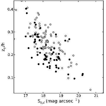
BM02 analyzed a sample of late-type edge-on galaxies in the $J$, $H$ and $K_{\mathrm{s}}$ bands (see Table 1). They have noted a strong correlation between the central surface brightness of a stellar disc and the $h/z_{0}$ ratio. This means that the thinner a galaxy is, the lower its central surface brightness reduced to the face-on orientation $S_{\mathrm{0,d}}$ (we will designate the apparent central surface brightness of edge-on galaxies as $\mu_{\mathrm{0,d}}$). The same correlation was confirmed for the stellar disc structural parameters corrected for internal extinction (Bizyaev & Kajsin, 2004; BM09). Bizyaev & Kajsin (2004) noted that this extinction correction is rather small (the median value for their sample is about 0.1 mag/arcsec²). Fig. 2 demonstrates the $S_{0,d}$ – $z_{0}/h$ correlation. BM09 concluded that a very wide scatter of points in this correlation is due to the relatively low accuracy in the $\mu_{\mathrm{0,d}}$, $z_{0}$ and $h$ and is also due to the non-constant value of the mass-to-light ratio ($M/L$) for different galaxies.

Figure 2: Correlation between the relative thickness of a disc and its reduced central surface brightness in the $K_{\mathrm{s}}$ band. Data were taken from BM02. Black filled circles correspond to the more reliable subsample (designated as “x” in the table 1 from BM02).

3.3 How does the relation $S_{0,d}$ – $z_{0}/h$ reveal itself in other samples

The largest sample of edge-on galaxies with derived structural parameters of discs and bulges is the MSR10 sample (see Table 1). It comprises both early and late type objects. The fits-images were taken from 2MASS in all three bands ($J$, $H$ and $K_{\mathrm{s}}$). The sample is incomplete according to the $V/V_{\mathrm{max}}$ test, but the subsample of 92 galaxies with angular radius $r>60$ arcsec appears to be complete. The program BUDDA (Bulge/Disc Decomposition Analysis; de Souza, Gadotti & dos Anjos, 2004) was applied for performing bulge/disc decomposition. As we have all needed structural parameters, we can construct the same relation as in BM02.

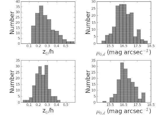
Let us compare the sample by MSR10 and the BM02 sample. In Fig. 3 we plotted the distributions of the parameters $z_{\mathrm{0}}/h$ and $\mu_{\mathrm{0,d}}$ in the $K_{\mathrm{s}}$ band. The BM02 sample comprises mainly late-type spiral galaxies. That is why the distributions over photometric parameters for this sample look slighlty different in comparison with our sample, but the mean values of both samples are similar.

The median values and standard deviations for the MSR10 sample are the following:

$$\langle z_{\mathrm{0}}/h\rangle=0.25\pm 0.11\,,$$

$$\langle\mu_{\mathrm{0,d}}\rangle=16.46\pm 0.69\,\mathrm{mag\,arcsec}^{-2}\,,$$

For the BM02 sample:

$$\langle z_{\mathrm{0}}/h\rangle=0.23\pm 0.07\,,$$

$$\langle\mu_{\mathrm{0,d}}\rangle=16.62\pm 0.56\,\mathrm{mag\,arcsec}^{-2}\,.$$

From these distributions we can see that the scatters of both parameters are relatively narrow, and the characteristics of the samples are close.

Figure 3: Distributions of the relative thickness and the deprojected central surface brighness of the discs in the $K_{\mathrm{s}}$ band for the sample by MSR10 (top plots) and for the BM02 sample (bottom plots).

In Fig. 4 we show the mutual distribution of $\mu_{\mathrm{0,d}}$ and $z_{\mathrm{0}}/h$ for our sample (row $a$, left plot) and for the BM02 sample (row $b$, left plot). Right plots in Fig. 4 represent the $S_{\mathrm{0,d}}$ – $z_{\mathrm{0}}/h$ correlation for our sample (row $a$) and for the BM02 sample (row $b$). The regression line for the MSR10 sample is

$$S_{\mathrm{0,d}}=-5.09\log(z_{0}/h)+14.81,\,r=-0.49\,,$$ (2)

and for the BM02 sample is

$$S_{\mathrm{0,d}}=-5.17\log(z_{0}/h)+14.71,\,r=-0.684\,.$$ (3)

Correlations for both samples are similar and rather strong, but are they real?

It is known from the surface photometry of transparent discs that the central surface brightness of the face-on disc (when the inclination angle is $i=0^{\circ}$) expressed in magnitudes per arcsec², can be reduced from the edge-on (apparent) central surface brightness as follows:

$$S_{\mathrm{0,d}}=\mu_{\mathrm{0,d}}-2.5\,\log(z_{0}/h).\,$$ (4)

From this expression (4) we may notice several useful facts. First, the scatter of $S_{\mathrm{0,d}}$ should be larger than that of $\mu_{\mathrm{0,d}}$ because of the presence of the term $\log(z_{\mathrm{0}}/h)$. Second, from (4) we can see that if $z_{0}/h\approx\mathrm{const}$, then there is a simple linear dependence between $S_{\mathrm{0,d}}$ and $\mu_{\mathrm{0,d}}$. Third, contrary, if $\mu_{\mathrm{0,d}}\approx\mathrm{const}$, there is a simple logarithmic dependence between $S_{\mathrm{0,d}}$ and $z_{\mathrm{0}}/h$. Hence, the small scatters around the median values $\langle\mu_{\mathrm{0,d}}\rangle$ and $\langle z_{\mathrm{0}}/h\rangle$ may transform the reduction formula (4) into the self-correlation between $S_{\mathrm{0,d}}$ and $z_{0}/h$ because the expression for $S_{\mathrm{0,d}}$ contains the term of $z_{0}/h$. To prove this conclusion, we designed some examples. They show that under certain conditions, perfect (but entirely spurious) correlation is obtained between two parameters formed from random distributions.

3.4 Self-relation between central surface brightness and thickness: artificial samples

We generated several samples of artificial galaxies with normal distributions of observed parameters $\mu_{\mathrm{0,d}}$ and $z_{\mathrm{0}}/h$. Although the distributions of $\mu_{\mathrm{0,d}}$ and $z_{\mathrm{0}}/h$ are not normally distributed in reality (see Fig. 3), we use this simplification merely to show that the resultant correlation will be the same as that for the real data.

The sample #1 (filled circles in Fig. 4c, left plot) is built to imitate the real distribution similar to our and the BM02 samples with the following mean value of $\mu_{\mathrm{0,d}}$ and its standard $\sigma$:

$$\bar{\mu}_{\mathrm{0,d}}=16.5,\,\sigma=0.6\,\mathrm{mag\,arcsec}^{-2}\,.$$

The sample #2 (open circles in Fig. 4c, left plot) has a wider distribution over $\mu_{\mathrm{0,d}}$:

$$\bar{\mu}_{\mathrm{0,d}}=16.5,\,\sigma=1.1\,\mathrm{mag\,arcsec}^{-2}\,.$$

In both cases the distribution of $z_{\mathrm{0}}/h$ was the same:

$$\overline{z_{\mathrm{0}}/h}=0.25,\,\sigma=0.05\,.$$

We converted $\mu_{\mathrm{0,d}}$ into $S_{\mathrm{0,d}}$ according to (4) and plotted the relation $S_{\mathrm{0,d}}$ – $\log(z_{0}/h)$ (see the right column in Fig. 4). It appears to be linear with a scattering that is due to the scatter of $\mu_{\mathrm{0,d}}$ and $z_{\mathrm{0}}/h$. The regression line for the sample #1 is

$$S_{\mathrm{0,d}}=-3.96\log(z_{0}/h)+15.42,\,r=-0.545\,,$$ (5)

and the regression line for the sample #2 (with a wide distribution over $\mu_{\mathrm{0,d}}$) is

$$S_{\mathrm{0,d}}=-1.41\log(z_{0}/h)+17.17,\,r=-0.21\,.$$ (6)

The regression coefficient is much smaller for this broader distribution of $\mu_{\mathrm{0,d}}$ (the sample #2, Fig. 4c, right plot, open circles, dashed line). Thus, the correlation $S_{\mathrm{0,d}}$ –$z_{0}/h$ for this sample is statistically insignificant. But for the artificial sample #1 containing random (uncorrelated) distributions of $\mu_{\mathrm{0,d}}$ and $z_{0}/h$ the regression coefficient and the slope of the correlation $S_{\mathrm{0,d}}$ –$z_{0}/h$ (Fig. 4c, right plot, filled circles, solid line) are almost the same as that for the BM02 and MSR10 samples. Thus, we can see that even if we have no correlation between the visible surface brightness of the edge-on disc and its relative thickness, there would be, nevertheless, the correlation between the reduced central surface brightness and the relative thickness of the disc.

This correlation, however, can be substantially smoothed and even destroyed if the scatter of $\mu_{\mathrm{0,d}}$ is rather large. To demonstrate this fact, we constructed two additional artificial samples. The sample #3 (filled circles in Fig. 4d, left plot) has a very small scatter of the ratio $z_{\mathrm{0}}/h$ ($\sigma=0.05$) and a large scatter of $\mu_{\mathrm{0,d}}$ (as for the sample #1) with the same mean values. The sample #4 (open circles in Fig. 4d, left plot), contrary, has a very small scatter of the value $\mu_{\mathrm{0,d}}$ ($\sigma=0.2$) and a wide distribution over the ratio $z_{\mathrm{0}}/h$ ($\sigma=0.1$). As a consequence, the sample #3 do not show any correlation between $S_{\mathrm{0,d}}$ and $z_{0}/h$ (filled circles in Fig. 4d, right plot). In other words, if there is a narrow scatter of $z_{\mathrm{0}}/h$ with the same distribution of $\mu_{\mathrm{0,d}}$ as for the sample #1, then the $S_{\mathrm{0,d}}$ – $z_{\mathrm{0}}/h$ correlation does not appear.

On the contrary, if we have a large scatter of $z_{\mathrm{0}}/h$ with a very narrow distribution of $\mu_{\mathrm{0,d}}$, then the expected correlation will be very strong (open circles in Fig. 4d, right plot).

Figure 4: Correlations between the relative thickness and the central surface brightness ($K_{\mathrm{s}}$ band): apparent (left column) and reduced (right column); a) the sample by MSR10; b) the BM02 sample; c) artificial samples #1 and #2 (filled circles and open circles respectively); d) artificial samples #3 (filled circles) and #4 (open circles), see the text. Solid lines correspond to the regression lines for the samples mentioned in the text. Dashed line is a regression line for the sample #2.

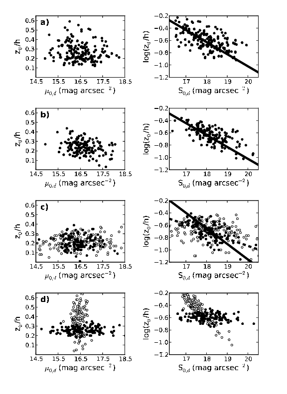
Trying to explain the $S_{\mathrm{0,d}}$ – $z_{0}/h$ correlation, Bizyaev & Kajsin (2004) noted that the values of $S_{\mathrm{0,d}}$ and $z_{0}/h$ had not been obtained independently from each other as can be concluded from the Eq. (4). They considered several effects that can affect the correlation $S_{\mathrm{0,d}}$ – $z_{0}/h$. In particular, they argue that a non 90 degree inclination of the disc simply shifts the data points in Fig. 4 towards the upper right corner because of the overestimation of $z_{0}$. Hence, systematic errors due to inclination may only scatter the dependence shown in Fig. 4 and do not affect a correlation if it exists. This explanation can not be adopted because there is certainly a scatter around the relation (4) with the median value of $\langle\mu_{\mathrm{0,d}}\rangle$. The slope of the regression lines (2) and (3) is twice as large as the slope of the relation (4) with the median value $\langle\mu_{\mathrm{0,d}}\rangle$, but the slope of the relation for artificial sample #1 is also larger (see the expression (5)). In other words, we can not assert the existence of the $S_{\mathrm{0,d}}$ – $z_{\mathrm{0}}/h$ correlation beyond the self-correlation due to the reduction procedure (4).

3.5 Are there physical bases of the correlation $S_{\mathrm{0,d}}$ – $z_{\mathrm{0}}/h$?

Let us turn to the possible explanation of the correlation $S_{\mathrm{0,d}}$ – $z_{\mathrm{0}}/h$, if it exists. Following BM09 (see also Zasov et al., 2002; , 2005; Sotnikova & Rodionov, 2006), we will consider the exponential disc which is in equilibrium in the vertical direction. For such a disc we can find the vertical scaleheight $z_{0}$ via the vertical equilibrium condition for an isothermal slab (Spitzer, 1942): $\sigma_{z}^{2}=\pi G\Sigma z_{0}$, where $\sigma_{z}$ is the vertical velocity dispersion, and $\Sigma$ is the surface density of a slab. To express the central surface density through the central surface brightness, we can write: $\Sigma_{0}\propto 10^{-0.4S_{\mathrm{0,d}}}$. The mass of the disc can be estimated as $M_{\mathrm{d}}=2\pi\Sigma_{\mathrm{0}}h^{2}$. At $R\simeq 2h$, the rotation curves of luminous galaxies generally reach a plateau. In the plateau region, the linear circular velocity $v_{\mathrm{c}}$ is roughly constant. We can then use $v_{\mathrm{c}}$ to estimate the total mass of a galaxy (including the mass of its spherical component: bulge$+$dark halo) within the sphere of the radius $R=4h$: $M_{\mathrm{tot}}(4h)=4v_{\mathrm{c}}^{2}h/G$. Thus, we have:

$$\frac{M_{\mathrm{tot}}(4h)}{M_{\mathrm{d}}}\propto\frac{v_{\mathrm{c}}^{2}}{h}10^{0.4S_{\mathrm{0,d}}}\,.$$ (7)

We can link the relative mass of a disc with its relative thickness via stability conditions. If the stellar disc is marginally stable in its plane, then the radial velocity dispersion can be written as $\sigma_{R}(R)=Q\,\displaystyle\frac{3.36G\,\Sigma(R)}{\kappa(R)}$, where $Q$ is the Toomre parameter (Toomre, 1964), $\kappa$ is the epicyclic frequency, $R$ is the radius in the cylindrical reference frame associated with the disc. For marginally stable discs the radial profile of $Q$ usually has a wide minimum with the value $Q\approx 1.5$ in the region of $(1-2)\cdot h$. This value is justified by the results of numerical experiments by Khoperskov et al. (2003). Thus, we can consider $Q$ to be almost constant with the radius outside the disc center. The epicyclic frequency at the region where $v_{\mathrm{c}}\approx\mathrm{const}$, is $\kappa\approx\sqrt{2}v_{\mathrm{c}}/R$. In summary, we obtain for $R\approx 2h$ (see Sotnikova & Rodionov, 2006 for details):

$$\frac{h}{z_{0}}\propto\frac{1}{\left(\sigma_{z}/\sigma_{R}\right)^{2}}\frac{v_{\mathrm{c}}^{2}/h}{\Sigma}\propto\frac{1}{\left(\sigma_{z}/\sigma_{R}\right)^{2}}\frac{M_{\mathrm{tot}}(4h)}{M_{\mathrm{d}}}\,.$$ (8)

If the ratio of vertical to radial velocity dispersions $\sigma_{z}/\sigma_{R}$ is almost constant throughout the disc, we have a correlation between $z_{\mathrm{0}}/h$ and $M_{\mathrm{d}}/M_{\mathrm{tot}}$. The existence of such a correlation was for the first time mentioned by Zasov, Makarov & Mikhailova (2002), and it was further explored in many works (e.g. Zasov et al., 2002; , 2005; Sotnikova & Rodionov, 2006; MSR10) and references in BM09). The ratio $\sigma_{z}/\sigma_{R}$ could be fixed at the level given by the local linear criterion for the marginal bending stability, i.e. at approximately 0.3 (Toomre, 1966; Kulsrud et al., 1971; Polyachenko & Shukhman, 1977; Araki, 1985). Recent numerical experiments by Rodionov & Sotnikova (2013) support this minimal value throughout the disc. For real galaxies, some mechanisms heating the disc in the vertical direction and causing an increase in the ratio $\sigma_{z}/\sigma_{R}$ may operate. At present, the ratio $\sigma_{z}/\sigma_{R}$ is measured directly only in a few galaxies (Gerssen et al., 1997, 2000; Shapiro et al., 2003; , 2012). It ranges from 0.3 to 0.8, but for our purposes we can fix this value at any level.

Now, combining (7) and (8) we can expect:

$$\frac{h}{z_{0}}\propto\frac{v_{\mathrm{c}}^{2}}{h}10^{0.4S_{\mathrm{0,d}}}\,.$$ (9)

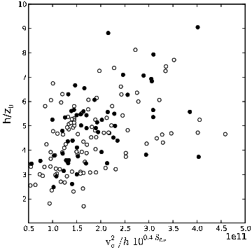
BM09 came to a similar conclusion. They used the correlation $h\sim v^{1.5}$ which they had observed, and found $z_{\mathrm{0}}/h\sim\Sigma_{0}/h^{1/3}$, where $\Sigma_{0}$ is the central surface density of a disc. They considered such a result to be the theoretical basis for their correlation between $h/z_{0}$ and $S_{\mathrm{0,d}}$ (BM02). We need to emphasize, however, that in the relation (9) we have not only the term $S_{\mathrm{0,d}}$ but also $v_{\mathrm{c}}^{2}/h$ (in the BM09’ version it is $h^{1/3}$). From this correlation it is not evident that there is a correlation between $S_{\mathrm{0,d}}$ and $(z_{0}/h)$ only! We may only conclude that there may be a correlation (9) which actually takes place as we can see in Fig. 5. Correlation (9), however, comprises the $S_{\mathrm{0,d}}$ term which was received via relation (4). Correlation (9), therefore, exists in the same sense as the correlation $S_{\mathrm{0,d}}$—$z_{0}/h$ exists. We can not prove the reality of this correlation for galaxies at moderate inclination for which $S_{\mathrm{0,d}}$ can be derived directly without reduction formula. Unfortunately, for such galaxies the ratio $z_{0}/h$ is undefined.

Moreover, the correlation between $z_{0}/h$ and $M_{\mathrm{d}}/M_{\mathrm{tot}}$ that was used to come to (9), is rather ambiguous, mainly due to the term $(\sigma_{z}/\sigma_{R})^{2}$ in the expression (8) (Sotnikova & Rodionov, 2006; MSR10). It exists only in the sense that discs embedded into very massive halos are always very thin.

3.6 Conclusion

The correlation between $h/z_{0}$ and $S_{\mathrm{0,d}}$, if it exists, is rather weak and can not be derived from observational data because the main effect seen in Fig. 4 is predominantly due to data reduction, many assumptions, and specific mathematical laws used to describe disc surface brightness distribution. All together, it gives a predictable result, i.e. a self-correlation.

Figure 5: Correlation between $z0/h$ and $v_{\mathrm{c}}^{2}/h\,10^{0.4S_{\mathrm{0,d}}}$ (which is proportional to $M_{\mathrm{d}}/M_{\mathrm{tot}}$) in the $K_{\mathrm{s}}$ band. Open circles represent the complete subsample of the sample by MSR10, filled circles represent the BM02 subsample. The rotational velocity values $v_{\mathrm{c}}$ were taken from the LEDA database (as uncorrected for inclination vmax output parameters supposing that the inclination $i\approx 90^{\circ}$ for all galaxies considered).

4 Bulges and ellipticals: Photometric Plane

4.1 Background

The overall shape of elliptical, dwarf elliptical and bulge profiles can be quantified and parametrized by means of $r^{1/n}$ law (Sérsic, 1968) for the radial surface brightness $I(r)$ which is a simple generalization of $r^{1/4}$ (de Vaucouleurs, 1948, 1953, 1959) and exponential laws by Freeman (1970) (see, for example, Davies et al., 1988; Young & Currie, 1994; Graham, 2001 and references therein).

The $r^{1/n}$ profile is given by the formula:

$$I(r)=I_{0}\,e^{-\nu_{n}(r/r_{\mathrm{e}})^{1/n}}\,,$$ (10)

where $r_{\mathrm{e}}$ is the effective radius, i.e. the radius of the isophote that contains 50% of the total luminosity of a galaxy or a bulge, $I_{0}$ is the central surface brightness, $n$ is the Sérsic index defining the shape of the profile, and the parameter $\nu_{n}$ ensures that $r_{\mathrm{e}}$ is the half-light radius. In magnitudes per arcsec² the expression (10) appears as follows

$$\mu(r)=\mu_{0}+\frac{2.5\,\nu_{n}}{\ln{10}}\,\left(\frac{r}{r_{\mathrm{e}}}\right)^{1/n}\,,$$ (11)

where $\mu_{0}$ is the central surface brightness expressed in mag per arcsec². The coefficient $\nu_{n}$ depends on $n$ and is an almost linear function of the Sérsic index $n$. As usual, one implies a numerical approximation of $n$ in any appropriate form. One of these approximatione which is valid in the range $0.5\leq n\leq 16.5$, is (, 1993)

$$\frac{\nu_{n}}{\ln{10}}\simeq 0.868\,n-0.142\,.$$ (12)

The profile of an elliptical galaxy (and a bulge of a spiral) that is fitted with the Sérsic model, can be also expressed as

$$\mu(r)=\mu_{\mathrm{e}}+1.0857\,\nu_{n}\left[\left(r/r_{\mathrm{e}}\right)^{1/n}-1\right]\,.$$ (13)

where $\mu_{\mathrm{e}}$ is the effective surface brightness, i.e. the surface brightness at $r_{\mathrm{e}}$.

For the fitting purpose, we can use the formula (11) and consider $\mu_{0}$ and $n$ as free (fit) parameters fixing the range of possible values of $\mu_{\mathrm{e}}$ (e.g. , 1993). In this case the uncertainty associated with the determination of $\mu_{\mathrm{e}}$ arises because $\mu_{\mathrm{e}}^{*}=\mu_{0}+1.0857\,\nu_{n}$ can differ from its measured value $\mu_{\mathrm{e}}$. The value of $\mu_{\mathrm{e}}^{*}$ can be further compared with the measured counterpart $\mu_{\mathrm{e}}$ to test the goodness of a fit. On the contrary, if a fit for a sample is ambiguous and comprises systematic errors, such errors may affect scaling relations.

In the bulge-disc decomposition, we have the following as free (fit) scaling parameters for a bulge: (1) the central bulge intensity $I_{\mathrm{0,b}}$ in counts what can be later converted to $\mu_{\mathrm{0,b}}$ in mag arcsec^-2; (2) the half-light radius of the bulge $r_{\mathrm{e}}$ in pixels; (3) the bulge shape parameter $n$ (e.g. , 2000b; Khosroshahi et al., 2004). In this case, $\mu_{\mathrm{e,b}}$ can be calculated from the expression

$$\mu_{\mathrm{e,b}}=\mu_{\mathrm{0,b}}+1.0857\,\nu_{\mathrm{n}}\,.$$ (14)

It has become customary to choose $\mu_{\mathrm{e,b}}$ as a fit scaling parameter instead of $\mu_{\mathrm{0,b}}$ (Möllenhoff & Heidt, 2001; MacArthur, Courteau & Holtzman, 2003; Balcells, Graham & Domínguez-Palmero, 2006; Méndez-Abreu et al., 2010; G09; MSR10). In this case, $\mu_{\mathrm{0,b}}$ is not an independent parameter but is calculated from the formula (14) that involves $n$.

4.2 Photometric Plane as a bivariate relation

The derived scaling parameters of galaxies may correlate. Correlations comprising the scaling parameters of Sérsic models, are widely discussed in the literature as well as the physical reasons of such correlations. Graham & Guzmán (2003) discussed several linear scaling relations for elliptical galaxies (mainly for dEs and intermediate to bright E galaxies). There are also bivariate correlations. One of them was introduced by Khosroshahi et al. (2000a) and (2000b) and was called Photometric Plane (PhP). Many authors have confirmed it for their samples of elliptical galaxies and bulges of spiral galaxies of all types in various bands (Möllenhoff & Heidt, 2001; Ravikumar et al., 2006; Méndez-Abreu et al., 2010; Laurikainen et al., 2010), in different environments (Khosroshahi et al., 2004), and for faint and bright objects (Barway et al., 2009).

(2000b) presented the PhP as a bivariate relation that links only photometric parameters obtained by fitting a Sérsic model to a galaxy image (or to a bulge), i.e. the Sérsic index $n$, the central surface brightness $\mu_{\mathrm{0,b}}$, and the effective radius of a galaxy, or of a bulge $r_{\mathrm{e,b}}$.

For any sample we can perform the least-squared fit of the expression

$$\log(n)=a\log(r_{\mathrm{e,b}})+b\,\mu_{\mathrm{0,b}}+c$$ (15)

and find $a$, $b$ and $c$. In the literature there are different versions of the Photometric Plane, and we refer to the plane in the form (15) as the PhP1.

(2000b) concluded that there exist two univariate correlations between the effective radius and the Sérsic index $n$, and between $n$ and the central surface brightness. These univariate correlations have a scatter that may be caused by a third parameter. The methods of multivariate statistics applied to the three parameters $n$, $\mu_{\mathrm{0,b}}$, and $r_{\mathrm{e,b}}$ may reduce the scatter and give the best-fit plane like that expressed by Eq. (15).

The Photometric Plane is thought to be a counterpart of a plane of a constant specific entropy of galaxies introduced by Lima Neto et al. (1999). Lima Neto et al. (1999) proposed two laws that elliptical galaxies and bulges of spirals must obey if they form and reach a quasi-equilibrium stage solely under the influence of gravitational processes. The first law is the virial theorem, and the second one is that a system in equilibrium is in a maximum entropy configuration.

Márquez et al. (2000, 2001) argued that after violent relaxation spherical systems may be considered to be in a quasi-equilibrium stage. In this stage, the two above mentioned laws are valid, and they lead to quasi-constant specific entropy. Ravikumar et al. (2006) expressed the specific entropy $S$ in a convenient form via three photometric parameters $\mu_{\mathrm{0,b}}$, $r_{\mathrm{e,b}}$ in kpc, and $n$. If $S=\mathrm{const}$, there exists the relation that connects only $\mu_{\mathrm{0,b}}$, $r_{\mathrm{e,b}}$ in kpc, and $n$. This relation gives the surface (plane) of a constant specific entropy. The value of specific entropy may be adjusted so to match the specific entropy plane with the Photometric Plane (see, for example, Khosroshahi et al., 2004; Ravikumar et al., 2006). Such a coincidence between two planes is thought to give a physical interpretation of the PhP1. The PhP1 may be understood as a consequence of the two laws mentioned above. A physical interpretation of the PhP1 given by Márquez et al. (2001), clarifies the processes that drove the formation and evolution of galaxies and proves that the PhP1 is not simply an artifact of the definitions of the photometric parameters.

4.3 Photometric Plane 1: is it flat?

In previous papers (MSR10; , 2012), we revealed that the PhP1 in $J$, $H$ and $K_{\mathrm{s}}$ bands appeared not to be flat. It has a prominent curvature towards small values of $n$ (with $\log(n)<0.2$). Such a curvature is not seen in early papers that used small samples with rather large values of $n$ (Khosroshahi et al., 2000a; , 2000b; Möllenhoff & Heidt, 2001), but it was noticed later (Khosroshahi et al., 2004; Ravikumar et al., 2006; Barway et al., 2009) and discussed in terms of a curved specific entropy surface. We consider the reason for this curvature to be quite a different one, and it helps to understand the origin of the relation (15).

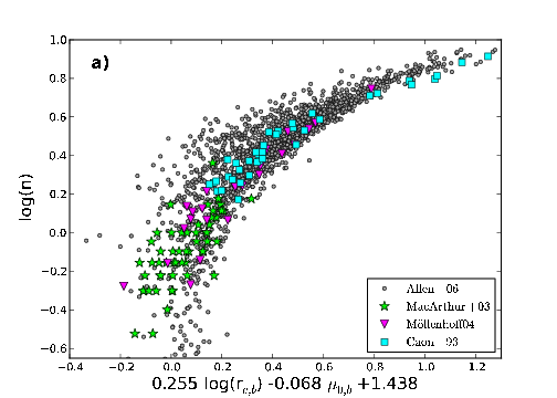
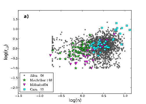
To clarify the question, we found the coefficients of the expression (15) and constructed the PhP1 (Fig. 6a) in the $B$ band for more than 10 000 galaxies of all types from the Millennium Galaxy Catalogue — MGC (Allen et al., 2006). We superimposed on this plane 45 intermediate to bright E galaxies from (1993). All these samples contain values of $\mu_{0}$, either fitted or recalculated from the model. We also added two samples containing structural parameters for bulges in the $B$ band: 121 face-on galaxies of late types from MacArthur, Courteau & Holtzman (2003) and 26 non-barred bright galaxies of all types from Möllenhoff (2004). We did not consider dwarf galaxies because their structure can differ substantially from the structure of bright ellipticals and bulges. At the same time, we consider bulges and elliptical galaxies all together. We will superimpose them often on the same plots keeping in mind that these are physically different objects. We are inetersted here only in the studying the shape of constructed correlations and dependencies which, as we could make sure, are similar for both elliptical galaxies and bulges from different samples (despite of their possible shift relative to each other on the plotted graphs).

We have mentioned that authors used different methods to calculate the distances to galaxies. The difference in distances may variate up to 10% and results in a slight difference of physical size of a galaxy. But when we compare different samples, we will consider the logarithm of the physical size of a component(for example, the effective radius of the bulge), so the scatter of its values for all the samples will be less in this scale and would not affect the shape of the relation.

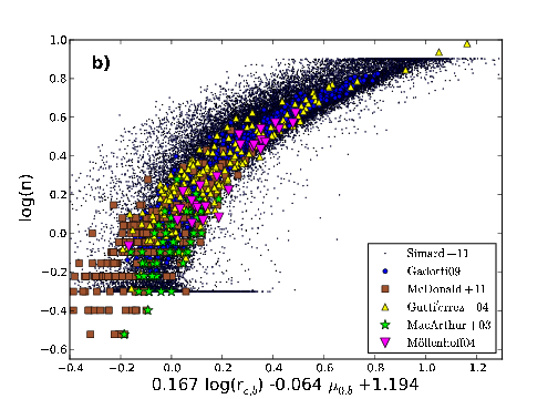
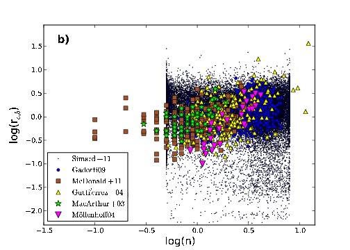
We constructed the same relation (Fig. 6b) in the $r$ band for the sample from Simard et al. (2011). The data for this sample comes from the Legacy area of the Sloan Digital Sky Survey Data Release Seven. This sample contains more than 1 million galaxies, sometimes very distant to be analyzed. Therefore we selected objects only with $0.02\leq z\leq 0.07$ (more than 200 000 galaxies). To avoid the presence of too many data points on our plots, we randomly selected 30 000 galaxies from the subsample. We also used a large sample of spiral and elliptical galaxies (946 objects) built by G09 where galaxies were originally selected with the same restriction on $z$. We added the sample of galaxies from the Virgo cluster (286 galaxies, McDonald et al., 2011) and 187 galaxies in a region of the Coma cluster (mainly Coma cluster members, , 2004). We added to these data 43 galaxies with known structural parameters from MacArthur, Courteau & Holtzman (2003) and galaxies from Möllenhoff (2004). All samples used in our analysis are listed in Table 2.

It turns out that for all samples there is a fairly tight correlation for bulges with $n\ga 2$ (classical bulges) and ellipticals, and a big scatter of points for bulges with $n\la 2$ (pseudobulges). The curvature of the PhP1 is also quite visible. The reason for the curvature may lie in the different nature of objects with $n\la 2$ and $n\ga 2$, or in something else.

Figure 6: The Photometric Plane (PhP1) constructed for a) the MGC sample (Allen et al., 2006) in the $B$ band; b) the subsample from Simard et al. (2011) in the $r$ band. Some other samples were superimposed on these planes (see the text and the legend).

4.4 Univariate relations

As was noted above, the bivariate correlation helps to diminish the scatter in univariate correlations. In our case, they are correlations between the Sérsic index $n$ and the central surface brightness, and between the effective radius and $n$. It is important to stress that a narrow plane connecting photometric parameters reveals itself only if the expression (15) comprises the central surface brightness $\mu_{\mathrm{0,b}}$. A corresponding plane does not appear if one uses $\mu_{\mathrm{e,b}}$ instead of $\mu_{\mathrm{0,b}}$ (see, for example, Möllenhoff & Heidt, 2001). Let us now consider two mentioned univariate relations.

4.4.1 Central surface brightness vs Sérsic index for bulges and ellipticals

Graham & Guzmán (2003) presented a tight linear relation between $\mu_{0}$ and $\log(n)$ (their figure 9f). The data have been compiled from several samples of elliptical galaxies (, 1993; Binggeli & Jerjen, 1998; Stiavelli et al., 2001; Graham & Guzmán, 2003) with derived structural parameters in the $B$ band (the Sérsic model was used). Such a correlation was noted as a very strong while analyzing data for elliptical dwarfs in the Coma cluster (Binggeli & Jerjen, 1998; Kourkchi et al., 2012).

Modeling the bulges of spiral galaxies, other authors have found a similar trend (e.g. , 2000b; Möllenhoff & Heidt, 2001; Aguerri et al., 2004; Ravikumar et al., 2006; Barway et al., 2009).

To explain this trend for dEs, Graham (2011, 2013a) discussed two key empirical linear relations from which the linear relation between $\mu_{0}$ and $\log(n)$ can be derived. They are the luminosity-concentration ($L-n$) relation and the luminosity-central density ($L-\mu_{0}$) relation which unify faint and bright elliptical galaxies along one linear sequence. This issue will be discussed in Section 5.

It should be noted that the points in figure 9f from Graham & Guzmán (2003) do go along a straight line, and the scatter looks natural because of inhomogeneity in the compiled sample and uncertainties while fitting photometric profiles. The deviation from the straight line is seen only at small values of $n$, but the sample in this range is poor (see also Graham, 2011, figure 2b).

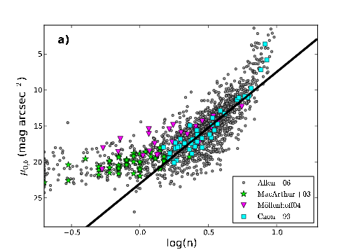
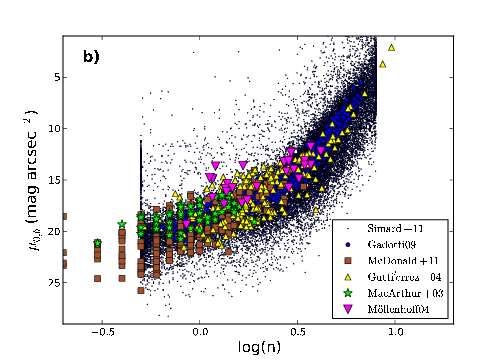
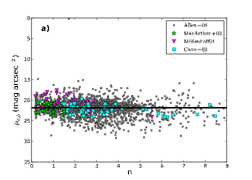
We reproduced the relation $\mu_{0}$ – $\log(n)$ in the $B$ band (Fig. 7a) and in the $r$ band (Fig. 7b) for all samples as in Fig. 6. The line $\mu_{0}=23-15.5\,\log(n)$ in Fig. 7a was drawn as in Graham (2011) where it has been estimated by eye. We also reproduced the relation $\mu_{0}$ – $\log(n)$ in the $r$ band separately for the sample by G09 in the Fig. 18 while discussing the Kormendy relation. For both bands the relation $\mu_{0}$ – $\log(n)$ clearly curves towards the range of small values of $n$ and does not follow a straight line.

Figure 7: The central surface brightness $\mu_{\mathrm{0,b}}$ of the underlying host galaxy bulge or of the elliptical shown against the Sérsic index $n$ on a logarithmic axis; a) the data are in the $B$ band where the solid line corresponds to the relation $\mu_{0}=23-15.5\,\log(n)$ from Graham (2011); b) the data were taken in the $r$ band (the data of G09 are reproduced separetly in Fig. 18 and in Fig. 20, where they are plotted with $n$ instead of $\log(n)$). The samples used are listed in Table 2.

4.4.2 Discussion and explanation

Several questions arise. Why is this relation curved? Is it real? Does it reflect some common physical processes which make spherical galaxies and bulges acquire their structure? Or, on the contrary, can this relation be explained simply by the procedure of image decomposition and surface brightness profile fitting?

To sort out these questions, let us first consider the relation $\mu_{\mathrm{e,b}}$ vs $n$. Surprisingly, being primarily measured (as for ellipticals) or fitted (as for bulges), $\mu_{\mathrm{e,b}}$ shows no trend with $n$. The top plot in Fig. 8 demonstrates data from several samples of elliptical galaxies and of spiral galaxy bulges in the $B$ band. The compiled sample is inhomogeneous; the scatter is large. Some points fall off the main distribution. This is a case of bright galaxies by Möllenhoff (2004). But both for the entire sample and for each subsample we can not observe the trend. The lack of the trend clearly manifests itself for the largest sample of galaxies from MGC. The sample is poorly inhabited in the region of large values of $n$, but the general behaviour is unambiguous. The straight line shows the median value of $\mu_{\mathrm{e,b}}$ for MGC’s galaxies. Bright galaxies from Möllenhoff (2004) are above this line contributing only to the scatter, but without creating the trend.

Figure 8: The effective surface brightness $\mu_{\mathrm{e,b}}$ of the underlying host galaxy bulge or of the elliptical shown against the Sérsic indices $n$; a) the data are in the $B$ band, $\langle\mu_{\mathrm{e,b}}\rangle=21.81$ mag arcsec^-2 corresponds to the MGC sample; b) the data were taken in the $r$ band, $\langle\mu_{\mathrm{e,b}}\rangle=20.48$ mag arcsec^-2 corresponds to the Simard et al. (2011) subsample. In order to show the lack of trend of $\mu_{\mathrm{e,b}}$ with $n$ for the Simard et al. (2011) subsample, the values of $\mu_{\mathrm{e,b}}$ were avaraged inside the bin $\Delta n=0.5$. The corresponding bars represent the standard deviation of $\mu_{\mathrm{e,b}}$ inside each bin. The samples used are listed in Table 2.

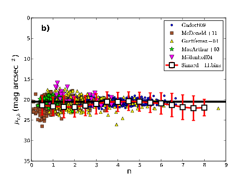
The most impressive example is shown in Fig. 8b. It shows the data in the $r$ band for the bulges from the sample by Simard et al. (2011). The data were complemented by several additional samples with available decompositions in the same $r$ band as in Fig. 7b. In Fig. 8b the data from the very homogeneous sample of spiral galaxies by G09 are also plotted. It is clearly seen that the points merely scatter around the median value of $\mu_{\mathrm{e,b}}$ (straight line). There is no trend of $\mu_{\mathrm{e,b}}$ with $n$. There is a slight bend around the median value of $\mu_{\mathrm{e,b}}$ for Simard’s (2011) data. The procedure of $\mu_{\mathrm{e,b}}$ deriving is not direct for this sample, and the fitting procedure itself can be a reason of existence of that bend. Faint Virgo cluster galaxies (McDonald et al., 2011) and bright galaxies from Möllenhoff (2004) deviate from the straight line lying above and below the median line.

The lack of the trend of $\mu_{\mathrm{e,b}}$ with $n$ was neither noted nor discussed earlier but helps us to understand the relation between $\mu_{\mathrm{0}}$ and $n$. As $\nu_{\mathrm{n}}$ is an almost linear function of $n$ (see Eq. 12), $\mu_{\mathrm{0,b}}$ can be expressed as:

$$\mu_{\mathrm{0,b}}\sim\langle\mu_{\mathrm{e,b}}\rangle-1.0857\,(2n-0.33)\,,$$ (16)

where $\langle\mu_{\mathrm{e,b}}\rangle$ is the median value for a sample. This is a linear self-relation between $\mu_{\mathrm{0,b}}$ and $n$.

As $\nu_{n}$ is an almost linear function of $n$ (see Eq. (12)), we have a linear self-relation between $\mu_{\mathrm{0,b}}$ and $n$ (see Fig. 20 for the sample by G09) that transforms into a curved self-relation between $\mu_{\mathrm{0,b}}$ and $\log(n)$ (see Fig. 7 and Fig. 18).

4.4.3 The relation between central surface brightness and Sérsic index: the Gadotti’s sample

To prove the above conclusion, we analyzed carefully the fiducial sample by G09 (we will often address to this sample further and use the data from the $r$ band). This sample contains a large amount of objects which were selected and decomposed very carefully. Thus, the data can be considered as quite homogeneous. Here we present the distributions over fitted photometric parameters $r_{\mathrm{e,b}}$, $\mu_{\mathrm{e,b}}$, and $n$ for this sample, both for bulges and ellipticals. We divided the bulges into two subsamples (faint bulges with $M_{\mathrm{bulge}}\geq-19.3$ and bright bulges with $M_{\mathrm{bulge}}<-19.3$) and considered separetely elliptical galaxies for which the bulge-to-total ratio $B/T=1$. The distributions are shown in Fig. 9.

Figure 9: Distributions over parameters $r_{\mathrm{e,b}}$, $\mu_{\mathrm{e,b}}$, and $n$ for the G09 sample. The division into three separate subsamples as it is found in G09. The black dashed line corresponds to faint bulges, the gray filled histogram is plotted for bright bulges, and the red solid line corresponds to elliptical galaxies. Vertical lines represent values of $r_{\mathrm{e,b}}=0.9$ kpc and $n=2.5$ to discriminate subsamples with bright and faint bulges.

The reasons for the division into subsamples were as follows. G09 showed that classical bulges ($n\ga 2$), pseudobulges ($n\la 2$), and bright elliptical galaxies are separate groups of objects. The most significant parameter separating these objects, is the Sérsic index $n$, and we can use boundary values of Sérsic model parameters distribution for several populations of objects. For the G09 sample there are two well visible peakes in distributions of $r_{\mathrm{e,b}}$ and $n$ (see Fig. 9). At the same time, the effective surface brightness distributions are similar for pseudobulges and classical bulges, and we can not distinguish the peaks of both distributions. We took the boundary values $r_{\mathrm{e,b}}\approx 0.9$ kpc, $\mu_{\mathrm{e,b}}\approx 20.2$ mag arcsec^-2 (median value for the subsample of bulges and pseudobulges), and $n\approx 2.5$. Then we put these values into the relation (see, for example, , 1994; Graham & Colless, 1997; Graham & Driver, 2005)

$$\begin{array}[]{rl}M_{\mathrm{bulge}}=\mu_{\mathrm{e,b}}&-2.5\log(ne^{\nu_{n}}\Gamma(2\,n)/\nu_{n}^{2\,n})-\\ &\\ &-2.5\,\log(2\pi r_{\mathrm{e,b}}^{2})-36.57\,,\\ \end{array}$$ (17)

As a result, we received $M_{\mathrm{sep}}\approx-19.3$ mag for the G09 sample.

Fig. 9 demonstrates three distinct populations of objects. The middle plot in Fig. 9 shows the distributions over $\mu_{\mathrm{e,b}}$. The overall range of $\mu_{\mathrm{e,b}}$ is rather small, no greater than 3 mag, but for each subsample the scatter is much smaller (about 1 mag). Thus, the distribution of $\mu_{\mathrm{e,b}}$ gives only the scatter around the relation (16) (see Fig. 10 which will be discussed below).

Figure 10: a) The dependence between the effective surface brightness $\mu_{\mathrm{e,b}}$ of the underlying host galaxy bulge or of the elliptical and the Sérsic index $n$; b) the linear relation between the central surface brightness $\mu_{\mathrm{0,b}}$ and the Sérsic index $n$. The data were taken from G09 ($r$ band). Black filled circles represent bright bulges ($M_{\mathrm{bulge}}<-19.3$ mag), black open circles represent faint bulges ($M_{\mathrm{bulge}}\geq-19.3$ mag), and red crosses correspond to elliptical galaxies. The solid line corresponds to the median value $\mu_{\mathrm{e,b}}\approx 20.2$ mag arcsec^-2 for the subsample of bulges and pseudobulges, the dash-dotted line corresponds to the median value $\mu_{\mathrm{e,b}}\approx 21.25$ mag arcsec^-2 for the subsample of ellipticals.

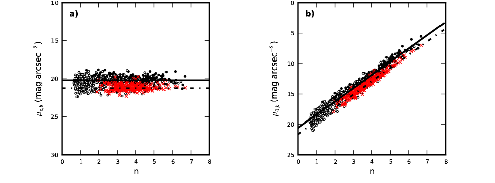
For small samples, the scatter around the relation between $\mu_{\mathrm{0,b}}$ and $n$ is small because of the limited range of $\mu_{\mathrm{e,b}}$ (as for subsamples of faint and bright bulges). The wider the distribution over $\mu_{\mathrm{e,b}}$ and the more inhomogeneous the compiled sample, the thicker the lane surrounding the relation (16) is, but the relation itself does not “sink” in the scatter.

In summary, there is no linear correlation between $\mu_{\mathrm{0,b}}$ and $\log(n)$. There is just an equality (14) which reflects the structure of the Sérsic model. The limited range of $\mu_{\mathrm{e,b}}$ for any sample transforms this equality into the linear pseudo-relation between $\mu_{\mathrm{0,b}}$ and $n$ (see Eq. (16)) creating a false illusion of a correlation, i.e a self-correlation. Moreover, at the limited range of $n$ any linear relation can be presented as logarithmic, i.e. depending on $\log(n)$. That is why there is no mystery in the widely discussed relation $\mu_{\mathrm{0,b}}$ vs $\log(n)$ (Binggeli & Jerjen, 1998; Khosroshahi et al., 2000a; , 2000b; Möllenhoff & Heidt, 2001; Graham & Guzmán, 2003; Aguerri et al., 2004; Ravikumar et al., 2006; Barway et al., 2009; Kourkchi et al., 2012). The relation is simply the result of a fitting procedure and is based on the formula (10) for the Sérsic surface brightness profile.

A self-correlation between $\mu_{\mathrm{0,b}}$ and $n$ follows from the fact that $\mu_{\mathrm{e,b}}$ is independent on $n$ that is well shown for G09 sample in Fig. 10a. Bulges, pseudobulges, and elliptical galaxies do not show any trend between $\mu_{\mathrm{e,b}}$ and $n$. Such an independence transforms into the linear pseudo-relation (Fig. 10b) between $\mu_{\mathrm{0,b}}$ and $n$ with a scatter that reflects the range of $\mu_{\mathrm{e,b}}$ in the samples under discussion. If we use $\log(n)$ instead of $n$, we obtain a curved pseudo-relation (Fig. 7). The nature of the curvature in Fig. 6 is exactly the same. The PhP1 includes $\mu_{\mathrm{0,b}}$ which according to (14) comprises $n$. We can approximate $n\sim\log(n)$ in a limited range of $n$ and obtain a nearly flat photometric plane in the form (15). In the wider range of $n$ it is curved (Fig. 7) because the relation between $\mu_{\mathrm{0,b}}$ and $n$ is linear (Fig. 10). In the next section, we show that the parameter $r_{\mathrm{e,b}}$ involved in the relation (15) does not affect our conclusion.

4.4.4 Effective radius vs Sérsic index for bulges and ellipticals

The existence of the univariate correlation between $r_{\mathrm{e,b}}$ and $n$ that might diminish the scatter in the bivariate relation, is very doubtful. Some authors revealed a correlation between $r_{\mathrm{e,b}}$ and $n$ (, 1993; Graham et al., 1996; , 2004; Möllenhoff, 2004; La Barbera et al., 2004, 2005). (2000b) and Möllenhoff & Heidt (2001) give the linear correlation coefficient for this correlation to be $\rho>0.6$ with a significance level of 99.98 %. Méndez-Abreu et al. (2010) were less enthusiastic about this correlation and estimated $\rho=0.28$ for their sample of S0-Sb galaxies in the $J$ band. Aguerri et al. (2004) analyzed the photometry of 116 bright galaxies from the Coma cluster and found the relation between $r_{\mathrm{e,b}}$ and $n$ to be statistically insignificant ($\rho=0.46$, $P=0.07$). Ravikumar et al. (2006) demonstrated that a plot of the Sérsic index against the effective radius shows the presence of two broad distributions (for Es and bright bulges, for dEs and faint bulges of S0s and spirals), but without a good correlation within each group. Barway et al. (2009) found systematic differences between bright and faint lenticulars with respect to the Sérsic index as a function of the effective radius. Bright lenticulars are well correlated ($\rho=0.79$ with significance greater than 99.99 %), but faint lenticulars do not show any correlation.

G09 sorted out the question about the correlation between $r_{\mathrm{e,b}}$ and $n$. He demonstrated that systems with larger $n$ tend to be more extended but this tendency is rather weak. The Sérsic index $n$ does slowly rise with $r_{\mathrm{e,b}}$ for bulges, but it is rather constant for ellipticals.

We replotted these correlations for the sample by G09 in the $r$ band. Fig. 11 represents the plane $r_{\mathrm{e,b}}$ – $n$. One can see that objects from three groups (faint bulges, bright bulges, and ellipticals) occupy quite different areas in Fig. 11. Bulges and elliptical galaxies are almost perpendicular to each other.

Figure 11: The dependence between the bulge effective radius and the Sérsic index plotted for the sample by G09 in the $r$ band (symbols as in Fig. 10).

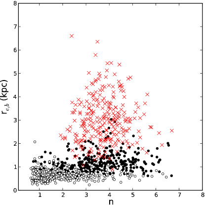
For bulges (rather faint objects) the scatter of $r_{\mathrm{e,b}}$ is small. On the contrary, the range of $n$ is large. Thus, the effective radius is almost independent on $n$. At the same time, bright galaxies (ellipticals) barely show the trend of $r_{\mathrm{e,b}}$ with $n$ along the wide area that is almost perpendicular to the $n$ axis. An inhomogeneous sample containing the random mixture of bulges and ellipticals, faint and bright objects can produce the false correlation between $r_{\mathrm{e,b}}$ and $n$.

Additionally, we have gathered data from the samples listed in Table 2 and plotted $r_{\mathrm{e,b}}$ against $n$ in the $B$ and $r$ bands (Fig. 12). The result is very convincing. One can notice a slight trend only for small samples, but the overall picture does not show any correlation.

Figure 12: The effective radius versus the Sérsic index for a) the $B$ band; b) the $r$ band. The samples used are listed in Table 2.

Here, it should be noted that we might be missing a significant part of galaxies with small bulges. The selection effects may put a low limit on the distribution of $r_{\mathrm{e,b}}$ which may change the view of found (or unfound) correlations. However, in this paper we do not consider the inhomogeneity or the completness of the samples.

Thus, the effective radius is not a third parameter that can improve the relation (15). Moreover, in the relation (15) $r_{\mathrm{e,b}}$ is expressed in kpc, so the term with $\log(r_{\mathrm{e,b}})$ can give a very small contribution in the $x$-axis expression presented in Fig. 6, and the leading relation in the expression (15) is a self-correlation (16).

4.5 Photometric Plane 1 as a self-relation

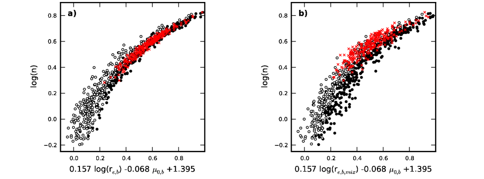
To demonstrate the insignificance of the contribution of the term with $r_{\mathrm{e,b}}$ which inputs only noise in the relation (18), we constructed the PhP1 for the G09 sample (Fig. 13a). For the overall sample we fitted the expression for the PhP1 as:

$$\log(n)=0.157\log(r_{\mathrm{e,b}})-0.068\,\mu_{\mathrm{0,b}}+1.395\,.$$ (18)

In the relation (18) the contribution of the term with $r_{\mathrm{e,b}}$ even for large galaxies ($\log(r_{\mathrm{e,b}})\approx 0.5$) is smaller than the scatter due to $\Delta\mu_{\mathrm{e,b}}\approx 3^{m}$ (see Fig. 9). Using (16), we rewrote the relation (18) in the form

$$\log(n)=0.157\log\langle r_{\mathrm{e,b}}\rangle-0.068\langle\mu_{\mathrm{e,b}}\rangle+0.074\,\nu_{n}+1.11\,,$$ (19)

where $\langle r_{\mathrm{e,b}}\rangle$ and $\langle\mu_{\mathrm{e,b}}\rangle$ are the median values of the effective radius and of the effective surface brightness, respectively. Now one can see that the PhP1 is simply another representation of the self-correlation (14), and the curvature of the PhP1 just shows the curvature of the expression for $\mu_{\mathrm{0,b}}$ via $\log(n)$.

The following trick helps to prove our main idea. We replotted the PhP1 (Fig. 13b) with the same expression (18) but mixed $r_{\mathrm{e,b}}$ values. As it has been done earlier, we split up the sample into three groups of galaxies: faint bulges (with $M_{r}\geq-19.3$), bright bulges (with $M_{r}<-19.3$), and ellipticals. The scatter in Fig. 13b increased, mainly for bright and large galaxies with a wide range of $r_{\mathrm{e,b}}$, but the overall shape of the dependence did not change. The curvature of the relation remains the same because the leading and trivial relation (self-correlation) between $\mu_{\mathrm{0,b}}$ and $\log(n)$ is curved.

Figure 13: The Photometric Plane (PhP1) for the G09 sample in the $r$ band; a) real data; b) G09 sample but with randomly mixed values of $r_{\mathrm{e,b}}$ (symbols as in Fig. 10).

Ravikumar et al. (2006) and Barway et al. (2009) noticed that different objects (ellipticals, bulges, faint and bright galaxies) form different photometric planes with different thicknesses. They noted that ellipticals and bulges of bright lenticulars have a tight Photometric Plane (PhP1), and they connected this fact with processes that lead to relaxed objects. Now we can see that the main difference in the PhP1s for samples used in our analysis, is the difference in the median value of $\mu_{\mathrm{e,b}}$ which shifts the plane. The range of $\mu_{\mathrm{e,b}}$ defines the thickness of the plane.

Thus, there is no mystery in the existence of the PhP1 which is simply a self-correlation contaminated by the term $r_{\mathrm{e,b}}$.

In Fig. 6 the coefficient under the term $\mu_{\mathrm{0,b}}$ is about the same (0.064 – 0.068) in different bands while the coefficient under the term $r_{\mathrm{e,b}}$ varies substantially. This proves that the leading relation in the expression (15) is the linear dependence of $\mu_{\mathrm{0,b}}$ on $n$ with the proviso that $\mu_{\mathrm{e,b}}$ is independent on $n$. But two intriguing questions remain. Why is the range of $\mu_{\mathrm{e,b}}$ for different objects rather small (on average, not greater than $5^{m}$ while the luminosity can change up to 8–9 magnitudes), and why $\mu_{\mathrm{e,b}}$ does not correlate with $n$?

4.6 Photometric Plane 2

Using a sample of early-type galaxies from the Virgo and Fornax clusters with photometric parameters in the $B$ band, Graham (2002) constructed the Photometric Plane as a variant of the Fundamental Plane (Djorgovski & Davis, 1987; Dressler et al., 1987) in which the Sérsic index $n$ has replaced the central velocity dispersion

$$\log(r_{\mathrm{e,b}})=a\log(n)+b\langle\mu\rangle_{\mathrm{e,b}}+c\,,$$ (20)

where $\langle\mu\rangle_{\mathrm{e,b}}$ is the mean surface brightness within the effective half-light radius. The value of $\langle\mu\rangle_{\mathrm{e,b}}$ can be obtained from $\mu_{\mathrm{e,b}}$ following, for example, (1994) and Graham & Colless (1997):

$$\langle\mu\rangle_{\mathrm{e,b}}=\mu_{\mathrm{e,b}}-2.5\log(ne^{\nu_{n}}\Gamma(2\,n)/\nu_{n}^{2\,n})\,.$$ (21)

Graham (2002) was motivated by the fact that $n$ quantifies the degree of mass concentration of a galaxy, and the central velocity dispersion traces the mass of a galaxy. Both these quantities may correlate. Graham (2002) found such a correlation and introduced the Photometric Plane (PhP2 in our notation) in the form given by the expression (20). La Barbera et al. (2004, 2005) derived the similar Photometric Plane in the $K$ band for early-type galaxies in two rich clusters at $z\sim 2$ and $z\sim 3$.

Without the term $\log(n)$ the relation (20) is simply a version of the Kormendy relation which is a univariate relation between $\log(r_{\mathrm{e,b}})$ and $\langle\mu\rangle_{\mathrm{e,b}}$. If there is another univariate relation between $\log(r_{\mathrm{e,b}})$ and $\log(n)$, we can reduce the scatter by constructing the bivariate relation (20). Graham (2002) claimed that the scatter in $\log(r_{\mathrm{e,b}})$ about the $\log(r_{\mathrm{e,b}})$ – $\log(n)$ relation for the data analysed was 0.35 dex while the scatter for the Kormendy relation between $\log(r_{\mathrm{e,b}})$ and $\langle\mu\rangle_{\mathrm{e,b}}$ was 0.25 dex. Using all three photometric parameters resulted in a tighter correlation with the scatter of 0.125 dex, La Barbera et al. (2004, 2005) came to the similar conclusion.

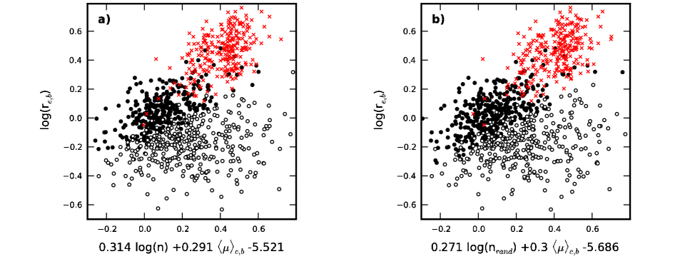
To check the above conclusion, we constructed the PhP2 in the form (20) for the G09 sample (Fig. 14a). Again, we distinguished between faint and bright bulges, and elliptical galaxies. We constructed PhP2 only for bright bulges and then superimposed on this plane all other galaxies from the G09 sample.

The scatter of points in Fig. 14a is very big. The relation is seen only for rather bright ellipticals and bulges (black filled circles).

First, this scatter is due to the lack of the correlation between $\log(r_{\mathrm{e,b}})$ and $\log(n)$ (see, for example, Figs. 11 and 12). Such a correlation reveals itself only for small samples, especially if they contain objects from the bottom left and top right corners as in Fig. 11, creating the illusion of the correlation. Secondly, the sample comprises faint objects that can deviate from the leading relation between $\log(r_{\mathrm{e,b}})$ and $\langle\mu\rangle_{\mathrm{e,b}}$.

To demonstrate the insignificance of the contribution of the term with $\log(n)$ in the relation (20), we took random values of $n$ for the the sample by G09 and reconstructed the PhP2 for bright objects (Fig. 14b) to compare it with the original data (Fig. 14a).

The most surprising thing is that the coefficient under the term $\langle\mu\rangle_{\mathrm{e,b}}$ retained its value, and it turned out to be robust. The coefficient under the term $\log(n)$ was slightly altered, but the overall picture did not change. This proves the littleness of the term $\log(n)$ in the relation (20).

Without the term of $\log(n)$ the relation (20) is a version of the Kormendy relation in which $\log(n)$ creates noise. Bright galaxies form a rather tight relation in Fig. 14a, and faint galaxies deviate from the relation in exactly the same way as in the Kormendy relation.

Figure 14: The Photometric Plane (PhP2) built for the sample by G09 in the $r$ band with true (a), i.e. taken from original papers, and random (b) values of the Sérsic index $n$. The limits of randomly taken $n$ were from 0.5 to 8 (symbols as in Fig. 10).

4.7 Photometric Plane 3

Kourkchi et al. (2012) used a sample of dwarf galaxies in the Coma cluster in magnitude range $-21<M_{I}<-15$ to construct the Photometric Plane in the form

$$\langle\mu\rangle_{\mathrm{e,b}}=a\log(r_{\mathrm{e,b}})+b\log(n)+c\,.$$ (22)

We designate this Photometric Plane as PhP3. The motivation of Kourkchi et al. (2012) was the same as in Graham (2002). They wanted to simplify the Fundamental Plane. Replacing the velocity dispersion with the Sérsic index, the PhP3 is obtained more economically than the Fundamental Plane because it is based only on photometric parameters. Kourkchi et al. (2012) also claimed that the scatter in the relation (22) diminished in comparison with two appropriate univariate relations.

As before, we constructed the PhP3 in the form (22) from the sample by G09 (Fig. 15a) with division into faint bulges, brigh bulges, and ellipticals. Objects from these three groups occupy quite different areas in Fig. 15a. Faint bulges have a larger scatter in the plane than bright bulges and ellipticals. The relation (22) comprises a weak self-correlation between $\langle\mu\rangle_{\mathrm{e,b}}$ and $n$ (see the relation (21)) which can affect the bivariate relation (22).

Figure 15: The Photometric Plane (PhP3) built for the sample by G09 in the $r$ band with true (a), i.e. taken from original papers, and random (b) values of the Sérsic index $n$ (symbols as in Fig. 10). The range of randomly taken $n$ was from 0.5 to 8.

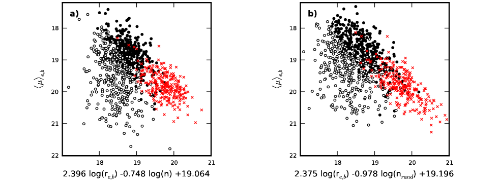
We destroyed this self-correlation by using random values of $n$. The reconstructed PhP3s are demonstrated in Fig. 15b. We can see that the term $\log(n)$ does not affect the overall shape of the relation, and it can be included in an arbitrary form. Thus, the relation (22) is a worse version of the Kormendy relation. It is not surprising that bright and faint bulges follow their own relations, and for the bright bulges the relation is tighter. The coefficient under the term with $\log(r_{\mathrm{e,b}})$ is about 2.4 which is close to the slope of the Kormendy relation.

4.8 Conclusion

In Sect. 4 we discussed various versions of the so-called Photometric Plane. This plane joins photometric characteristics ($n$, $\mu_{\mathrm{0,b}}$ or $\langle\mu\rangle_{\mathrm{e,b}}$, and $r_{\mathrm{e,b}}$.) of ellipticals and bulges of spiral galaxies.

As we have shown, the Photometric Plane has no independent physical sense — it simply reflects $\mu_{\mathrm{0,b}}$ – $n$ self-correlation (PhP1, Sect. 4.5) or is an entangled version of the Kormendy relation (PhP2 and PhP3, Sect. 4.6 and 4.7).

5 Kormendy relation

In this section we are about to touch on the essence of the above noted Kormendy relation which has being widely discussed for several decades.

5.1 Graham’s approach: outline

In some works we can find the idea that the Kormendy relation (and other similar to it curved relations between photometric parameters of ellipticals and of galaxy bulges) can not be considered as the evidence of the physical difference between dwarfs and bright ellipticals. The same issue stands for galaxies with pseudobulges and bright classical bulges. This point of view has been actively propagated by Graham in several articles (e.g. Graham & Guzmán, 2003; Graham, 2011, 2013a). His attempt to unify dwarfs and giant galaxies stems from the idea that the curved relations between photometric parameters are the result of the existence of two linear relations valid for both classes of objects. Graham’s conclusions were extended not only to elliptical galaxies, but also to disc galaxies with classical bulges and pseudobulges (Graham, 2013b). In this section we check these conclusions about the curved relations operating with the already used G09 sample as the best representative for bulges from our set of samples.

Graham (2011, 2013a) uses two main correlations between the Sérsic model parameters. These are the correlation between the luminosity and the central surface brightness of a spherical component (e.g. Binggeli & Jerjen, 1998; Graham & Guzmán, 2003), and the relation between the luminosity and the Sérsic index (e.g. , 1993; Young & Currie, 1994; Binggeli & Jerjen, 1998; Möllenhoff & Heidt, 2001; Graham & Guzmán, 2003; Ferrarese et al., 2006). In the $B$ band he found:

$$\begin{array}[]{l}M_{\mathrm{bulge}}=0.67\mu_{\mathrm{0,b}}-29.5\,,\\ M_{\mathrm{bulge}}=-9.4\log(n)-14.3\,.\\ \end{array}$$ (23)

From the above relations, Graham derived the expression between the central surface brightness and the Sérsic index:

$$\mu_{\mathrm{0,b}}=22.8-14.1\log(n)\,.$$

Graham (2013a) noted that this relation is roughly applicable only for values of $n\geq 1$ as one can see in fig. 7b from (Graham, 2013a).

5.2 The usage of Graham’s approach for the Gadotti’s sample

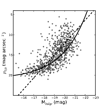
Let us follow the main idea of Graham (2013a) and derive two linear relations analogous to (23) but for the sample by G09. The distributions of the main photometric parameters are shown in Fig. 9. The univariate, namely, the relation between $\mu_{\mathrm{0,b}}$ and $M_{\mathrm{bulge}}$ is reproduced in Fig. 16 only for bulges. We found the regression line (dashed line) for the data. It corresponds to the expression

$$M_{\mathrm{bulge}}=0.35\,\mu_{\mathrm{0,b}}-24.23\,.$$ (24)

Figure 16: The correlation between the central surface brightness and the luminosity of bulges from the G09 sample in the $r$ band. The regression line (dashed line) corresponds to the relation (24) while the solid line refers to relations (25) and (29) .

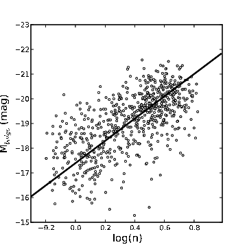
The relation between the Sérsic index and the luminosity is presented with the regression line (solid line) in Fig. 17, also only for bulges. We expressed the relation as:

$$M_{\mathrm{bulge}}=-4.51\,\log(n)-17.394\,.$$ (25)

Figure 17: The correlation between the luminosity and the Sérsic index (in the logarithmic scale) for bulges from the G09 sample in the $r$ band. The regression line corresponds to relation (25).

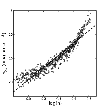
From these two relations one can derive:

$$\mu_{\mathrm{0,b}}=-12.88\,\log(n)+19.52\,,$$ (26)

The $\mu_{\mathrm{0,b}}$ – $n$ relation is presented in Fig. 18 with a regression line corresponding to the expression (26). Here we forget for a moment about our conclusion in Section 4.4.3 that this correlation is linear, but we will come back to this fact later.

Figure 18: The correlation between the central surface brightness and the Sérsic index (in the logarithmic scale) for bulges from the G09 sample in the $r$ band. The regression line corresponds to relation (26).

Then we can repeat the algorithm described in detail in Graham (2013a). We take the expression for $M_{\mathrm{bulge}}$ (it follows from Graham & Driver (2005)) as:

$$M_{\mathrm{bulge}}=\langle\mu\rangle_{\mathrm{e,b}}-2.5\,\log(2\pi r_{\mathrm{e,b}}^{2})-36.57\,,$$ (27)

where $\langle\mu\rangle_{\mathrm{e,b}}$ can be found from Eq. (21).

Now we can eliminate the absolute magnitude from the Eq. (27) replacing it from relation (24) where $\mu_{\mathrm{0,b}}$ can be expressed through $\langle\mu\rangle_{\mathrm{e,b}}$ from (21) and (14). At last, we will have the relation between $r_{\mathrm{e,b}}$ and $\mu_{\mathrm{e,b}}$ such that

$$\log(r_{\mathrm{e,b}})=0.2\,\left(0.56\,\mu_{\mathrm{e,b}}-A_{\mathrm{n}}-12.60+0.48\,\nu_{n}\right)\,,$$ (28)

where $A_{\mathrm{n}}=2.5\log(ne^{\nu_{n}}\Gamma(2\,n)/\nu_{n}^{2\,n})$.

Each value of $n$ can be associated with each value of $\mu_{\mathrm{e,b}}$ using relations (26) and (14). Thus, relation (28) is between $r_{\mathrm{e,b}}$ and $\mu_{\mathrm{e,b}}$ only. It is curved and shown in Fig. 19. Similar to this algorithm, we can build other curved relations such as $\langle\mu\rangle_{\mathrm{e,b}}$ – $r_{\mathrm{e,b}}$, $\mu_{\mathrm{e,b}}$ – $M_{\mathrm{bulge}}$, $\langle\mu\rangle_{\mathrm{e,b}}$ – $M_{\mathrm{bulge}}$, $r_{\mathrm{e,b}}$ – $M_{\mathrm{bulge}}$ (see Graham, 2013a).

Figure 19: The Kormendy relation for the bulges from the G09 sample in the $r$ band with superimposed relations constructed following Graham (2013a) and our approach (see the text). Symbols are as in Fig. 14. The line of gray filled circles represents the curved relation (28), the dashed red line is a relation for which $\mu_{\mathrm{e,b}}$ is recalculated according to (29) instead of (26) .

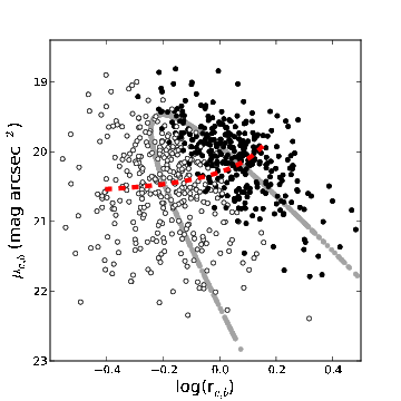
5.3 Our approach for the Gadotti’s sample

Let us now turn back to what we showed earlier in Section 4.4.3 where the true correlation between the central surface brightness and the Sérsic index appeared to be linear. For bulges from the sample by G09, this can be written as:

$$\mu_{\mathrm{0,b}}=-2.28\,n+20.96\,.$$ (29)

This relation is presented in Fig. 20.

Figure 20: The correlation between the central surface brightness of a bulge and the Sérsic index for the G09 sample in the $r$ band. The regression line corresponds to relation (29). Fig. 7 and Fig. 18 show the same with $\log(n)$.

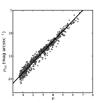
Earlier we showed that the effective brightness of elliptical galaxies and bulges does not depend on the Sérsic index, and for the subsample of bulges by the G09 sample the median value is $\langle\mu_{\mathrm{e,b}}\rangle=20.21$ mag arcsec^-2. Therefore, if we take relation (29) instead of (26), relation (25) presented in Fig. 17, and obtain the relation between $M_{\mathrm{bulge}}$ and $\mu_{\mathrm{0,b}}$, it will be curved. We marked this curved relation in Fig. 16 with the solid line. Surprisingly, this curved line represents the data better than the linear one and seems to be more appropriate to describe $\mu_{\mathrm{0,b}}$ – $M_{\mathrm{bulge}}$ correlation. Then, we can repeat the algorithm for building a relation between $\mu_{\mathrm{e,b}}$ and $r_{\mathrm{e,b}}$ and superimpose it on the data in the plane $\mu_{\mathrm{e,b}}$ – $r_{\mathrm{e,b}}$. This relation is shown in Fig. 19 as a black solid line. We can see that this relation does not describe the observed scatter of points at all and simply reflects the fact of independence of the parameter $\mu_{\mathrm{e,b}}$ on $n$.

From all of these facts we can conclude that at least for bulges presented in the sample by G09, the Graham’s approach is not applicable in order to explain the Kormendy relation by unifying it with two linear relations for faint and bright objects since one of them appeared to be wrong.

5.4 Another presentation of the Kormendy relation

Nonetheless, we shall try to apply another approach to check whether the Kormendy relation is real and does not follow from any unifying relations. To do this, we build several artificial samples which are described in Table 3. Here we suggest the detailed recipe how to construct the Kormendy relation and all other correlations for bulges and elliptical galaxies we have already discussed. We shall see that such relations have features of the real physical difference between galaxies with different photometric characteristics and the features of the embedded Sérsic law being used to describe a bulge component or an elliptical galaxy.

We consider distributions of the three Sérsic model parameters: $r_{\mathrm{e,b}}$, $\mu_{\mathrm{e,b}}$, and $n$ from the sample by G09. Let us note here that in this subsection we use the whole sample including elliptical galaxies. It is done to show more clearly our main idea about existence of curved relations (using wider ranges of all Sérsic model parameters). We start with the very simple case of uncorrelated parameters and end up with a sample similar to that which was investigated in G09.

Table 3: List of model samples created to illustrate the appearence of the curved relations. ‘True’ means original data column taken from G09, ‘mixed’ means randomly mixed data column, and ‘approx’ indicate that the parameter was found by using an approximation (see text).

Sample #	$\mu_{\mathrm{e,b}}$	$r_{\mathrm{e,b}}$	$n$	Comments	Correlations
0	true	true	true	G09 sample	All correlations from Gadotti (2009)
1	mixed	mixed	mixed	From G09	PhP1, $M_{b}$ vs $r_{\mathrm{e,b}}$
2	true	true	mixed	From G09	PhP1, all Kormendy relations
3	true	mixed	true	From G09	PhP1, $M_{b}$ vs $r_{\mathrm{e,b}}$
4	mixed	true	true	From G09	PhP1, $M_{b}$ vs $r_{\mathrm{e,b}}$, $M_{b}$ vs. $n$
5	approx	mixed	mixed	From G09, $\mu_{\mathrm{e,b}}$ built from (30)	PhP1, $M_{b}$ vs. $r_{\mathrm{e,b}}$, $M_{b}$ vs. $n$
6	approx	true	true	From G09, $\mu_{\mathrm{e,b}}$ built from (31)	All correlations from Gadotti (2009)

For the comparison, we plotted the correlations for the G09 sample (Fig. 21(0)) where the luminosity of the spheroidal component $M_{\mathrm{bulge}}$ was taken from the original tables of the decomposition results.

First, we consider the randomly mixed distribution of values for all three parameters from the sample by G09 (see Table 3, sample #1). It means that we randomly choose the values of this parameters from the G09 tables. We calculated the bulge total luminosity $M_{\mathrm{bulge}}$ via Eq. (17). It is evident that the Kormendy relation and different versions of it will not occur because $\mu_{\mathrm{e,b}}$ and $r_{\mathrm{e,b}}$ are not correlated. We can see in Fig. 21(1) that there is no correlation between the bulge total magnitude $M_{\mathrm{bulge}}$ and $\mu_{\mathrm{e,b}}$ as well as between $M_{\mathrm{bulge}}$ and the Sérsic index $n$. There is, however, a correlation $M_{\mathrm{bulge}}$ vs $r_{\mathrm{e,b}}$. The shape of this correlation differs from that valid for the sample by G09 (Fig. 21(0)).

We then build the samples with randomly mixed values of one parameter whereas other two parameters may correlate because they are taken from the real distributions (see Fig. 9). It means that we take values of two parameters for given galaxies as they are, and the third parameter is chosen randomly from the column containing this parameter (samples #2–#4). The luminosity of the spheroidal component $M_{\mathrm{bulge}}$ for samples #2–#4 was also calculated using Eq. 17. Some correlations can reveal themselves for such artificial samples, but others can be destroyed. For example, the Kormendy relation for correlated $r_{\mathrm{e,b}}$ and $\mu_{\mathrm{e,b}}$ (sample #2) keeps its shape (Fig. 21(2)), but it is completly pulled down for samples #3 and #4 (Fig. 21(3),(4)). The correlation $M_{\mathrm{bulge}}$ – $n$ disappears for samples #2 and #3 but is seen for sample #4.

To create the next sample #5, we take the mixed distributions of parameters from the $r_{\mathrm{e,b}}$ – $n$ plane while values of $\mu_{\mathrm{e,b}}$ are calculated from the Eqs. (27) and (21) where $M_{\mathrm{bulge}}$ is approximated (fitted) for sample #1:

$$M_{\mathrm{bulge}}=-4.62\,\log(r_{\mathrm{e,b}}-0.24)-19.775\,.$$ (30)

The line corresponding to this equation is presented in Fig. 21(1) on the second left plot. In Fig. 21(5) one can see that there is something similar to the Kormendy relation, but it is quite corrupted while the correlation $M_{\mathrm{bulge}}$ vs $n$ has not yet appeared.

At last, we take the same distribution of parameters from the $r_{\mathrm{e,b}}$ – $n$ plane as for sample #4 (i.e. as for the G09 sample), but $\mu_{\mathrm{e,b}}$ is calculated from the Eq. (27) where $M_{\mathrm{bulge}}$ is found (fitted) from the true correlation for the sample by G09 (see the solid line in Fig. 21(0), second left plot):

$$M_{\mathrm{bulge}}=-3.04\,\log(r_{\mathrm{e,b}}-0.38)-20.03\,.$$ (31)

As we discussed earlier (see Fig. 11), the distribution of galaxies in the $r_{\mathrm{e,b}}$ – $n$ plane represents two perpendicular subsystems: classical bulges + ellipticals and pseudobulges. This distribution is actually trimodal (see Fig. 9) that is very important for understanding curved relations as we shall see below.

In Fig. 21(6) it is apparent that for the last artificial sample #6 the built correlations resemble the correlations for the G09 sample very well. Therefore, these correlations can be reproduced only when the observed trimodal galaxy distribution in the $r_{\mathrm{e,b}}$ – $n$ plane (see Fig. 11) and the observed average scaling relation between $r_{\mathrm{e,b}}$ and $M_{\mathrm{bulge}}$ are assumed.

Figure 21: Correlations between some photometric parameters plotted for samples from Table 3. Each row represents one sample (row marked as “0” represents the distributions for the G09 sample). Red filled stars represent faint bulges ($M_{\mathrm{bulge}}\geq-19.3$ mag) and grey circles represent bright bulges and elliptical galaxies ($M_{\mathrm{bulge}}<-19.3$ mag). The solid lines are described in the text.

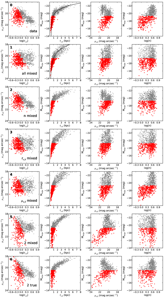
Let us now consider these correlations in more detail. The correlation $M_{\mathrm{bulge}}$ – $r_{\mathrm{e,b}}$ exists for all samples (even for randomly mixed parameter values) because of the presence of the term $r^{2}_{\mathrm{e,b}}$ in Eq. (27). Nevertheless, Fig. 22 shows explicitly that the true distribution of galaxies in the $M_{\mathrm{bulge}}$ – $r_{\mathrm{e,b}}$ plane (i.e. sample #0) can not be described using only Eq. (27). The correlation (31) for the last sample #6 has a slightly different form than for other samples. In Fig. 22, one can see the difference between the shape of the $M_{\mathrm{bulge}}$ – $r_{\mathrm{e,b}}$ correlation for samples #5 and  #6. The distribution of points in the $M_{\mathrm{bulge}}$ – $r_{\mathrm{e,b}}$ plane for sample #6 represents the true variety of galaxies (comparing with sample #0) what implies that the parameters $r_{\mathrm{e,b}}$, $\mu_{\mathrm{e,b}}$, and $n$ are correlated in a certain way.

Figure 22: Comparison between the two relations (31) and (30). Red open circles correspond to the data from the G09 sample in the $r$ band, blue filled circles correspond to sample #1. Solid and dashed lines represent the approximation of the data for the G09 sample and sample #1, respectively (Eqs. (31) and (30)).

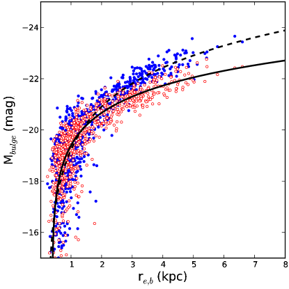
The Kormendy relation $\mu_{\mathrm{e,b}}$  – $r_{\mathrm{e,b}}$ appeares because of the same fact. The specific form of the correlation between $M_{\mathrm{bulge}}$ and $r_{\mathrm{e,b}}$ generates the curved relation between $\mu_{\mathrm{e,b}}$ and $r_{\mathrm{e,b}}$. The correlation $M_{\mathrm{bulge}}$ – $\mu_{\mathrm{e,b}}$, in turn, can be retrieved as a consequence of existing correlation $\mu_{\mathrm{e,b}}$  – $r_{\mathrm{e,b}}$ as follows from the consideration of sample #2, where $\mu_{\mathrm{e,b}}$ and $r_{\mathrm{e,b}}$ are correlated, and $n$ is a randomly mixed column. Thus, $M_{\mathrm{bulge}}$ – $r_{\mathrm{e,b}}$ relation as well as $M_{\mathrm{bulge}}$ – $\mu_{\mathrm{e,b}}$ relation is another representation of the Kormendy relation.

The correlation $M_{\mathrm{bulge}}$ – $n$ is a consequence of the bimodality of $n$ and $r_{\mathrm{e,b}}$. It is well seen that bright bulges and elliptical galaxies have little scatter of $n$ with the mean value of about 3.4 and the mean effective radius larger than that for faint bulges (Fig. 9). The population of faint bulges has a wider distribution of $n$ with smaller values of effective radius. Thus, we have two almost perpendicular subsystems in the plane $r_{\mathrm{e,b}}$ – $n$. These two clouds are also presented in the $M_{\mathrm{bulge}}$ – $n$ plane where bright bulges and elliptical galaxies lie in the upper right corner, while faint bulges are in the bottom left corner (see Fig. 21). If we had only galaxies with $M_{\mathrm{bulge}}\geq-19.3$ or $M_{\mathrm{bulge}}<-19.3$, the $M_{\mathrm{bulge}}$ – $n$ correlation would not be appear! These two separate clouds in the $M_{\mathrm{bulge}}$ – $n$ plane reveal the correlation between these two parameters.

Thus, the curved nature of the considered relations stems from the physical difference between faint and bright bulges. ‘Unifying’ curved relations of the kind of the grey line shown in Fig. 19 are the result of the hidden functional correlations of the main fitting parameters $r_{\mathrm{e,b}}$, $\mu_{\mathrm{e,b}}$, and $n$, combined with the intrinsic bi- or three modality of their true distributions.

6 Conclusions

We presented the results of the critical review of some widely discussed correlations between bulge and disc structural parameters, in different photometric bands and of various morphology. The main conclusions we can draw from this work can be summarized as follows:

1. The correlation between the edge-on disc central surface brightness reduced to the face-on view and the relative thickness of the stellar disc is a self-correlation. It can not empirically confirm that faint discs are, on average, more thin than discs of higher surface brightness. This correlation only appears as the consequence of application of the transparent exponential disc model and reflects the distribution characteristics of the sample studied.

2. There is no correlation between the effective surface brightness $\mu_{\mathrm{e,b}}$ and the Sérsic index $n$ for both bulges of spiral galaxies and ellipticals. The range of $\mu_{\mathrm{e,b}}$ for different type objects is rather small (not greater than 5^m for bulges and elliptical galaxies excluding dEs).

3. The Photometric Planes 1, 2, and 3 we considered, are relations between Sérsic model parameters which do not reveal anything new about bulges and elliptical galaxies. The PhP1 is a worse representation of the $\mu_{\mathrm{0,b}}$ – $n$ self-correlation that arises as a consequence of not only using the Sérsic law, but also of the independence of the effective surface brightness from the Sérsic index and a small range of the effective surface brightness regardless of the objects considered. The PhP2 and PhP3 are another (noisy) version of the Kormendy relation and do not give any new information about the structure of bulges and elliptical galaxies.

4. The Kormendy relation is a true correlation between main photometric parameters of bulges and elliptical galaxies which does help to divide galaxies into several populations. Classical bulges, pseudo-bulges, and elliptical galaxies have different origins and can not be described by curved relations proposed in Graham & Guzmán (2003); Graham (2011, 2013a). The bimodality of bulge parameters (or even trimodality, including elliptical galaxies) is a real observational fact.

   We end by warning the readers when dealing with  correlations between quantities depending on hidden common parameters.

References

- Aguerri et al. (2004) Aguerri J.A.L, Iglesias-Paramo J., Vilchez J.M., Munõs-Tuñón C., 2004, AJ, 127, 1344
- Allen et al. (2006) Allen P.D, Driver S.P., Graham A.W., Cameron E., Liske J., De Propris R., 2006, MNRAS, 371, 2
- Araki (1985) Araki S., A Theoretical Study of the Stability of Disk Galaxies and Planetary Rings, PhD Thesis, Massachus. Inst. Tech., 1985
- Balcells, Graham & Domínguez-Palmero (2006) Balcells M., Graham A.W., Domínguez-Palmero L., 2003, ApJ, 582, L79
- Barway et al. (2009) Barway S., Wadadekar Y., Kembhavi A.K., Mayya Y.D., 2009, MNRAS, 394, 1991
- Bedregal, Aragon-Salamanca & Merrifield (2006) Bedregal A.G., Aragon-Salamanca A., Merrifield M.R., 2006, MNRAS, 373, 1125
- Binggeli & Jerjen (1998) Binggeli B., Jerjen H., 1998, A&A, 333, 17
- Bizyaev & Mitronova (2002) Bizyaev D., Mitronova S., 2002, A&A, 389, 795 (BM02)
- Bizyaev & Kajsin (2004) Bizyaev D., Kajsin S., 2004, ApJ, 613, 886
- Bizyaev & Mitronova (2009) Bizyaev D., Mitronova S., 2009, ApJ, 702, 1567 (BM09)
- (11) Caon N., Capaccioli M., D’Onofrio M., 1993, MNRAS, 265, 1013
- (12) Caon N., Capaccioli M., D’Onofrio M., 1994, A&A, 286, 39
- Courteau et al. (2007) Courteau S., Dutton A.A., van den Bosch F.C., MacArthur L.A., Dekel A., McIntosh D.H., Dale D.A., 2007, ApJ, 671, 203
- Davies et al. (1988) Davies J.I., Phillipps S., Cawson M.G.M., Disney M.J., Kibblewhite E.J., 1988, MNRAS, 232, 239
- de Grijs (1998) de Grijs R., 1998, MNRAS, 299, 595
- de Jong (1996) de Jong R.S., 1996, A&A, 313, 45
- de Vaucouleurs (1948) de Vaucouleurs, 1948, Annales d’Astrophysique, 11, 247
- de Vaucouleurs (1953) de Vaucouleurs, 1953, MNRAS, 113, 134
- de Vaucouleurs (1959) de Vaucouleurs, 1959, Hdb. d. Physik, 53, 311
- de Souza, Gadotti & dos Anjos (2004) de Souza R.E., Gadotti D.A., dos Anjos S., 2004, ApJS, 153, 411
- Djorgovski & Davis (1987) Djorgovski S., Davis M., 1987, ApJ, 313, 59
- Dong & de Robertis (2006) Dong X.Y., de Robertis M.M., 2006, AJ, 131, 1236
- Dressler et al. (1987) Dressler A., Linden-Bell D., Burstein D., Davies R.L., Faber S.M., Terlevich R., Wegner G., 1987, ApJ, 313, 42
- Faber & Jackson (1976) Faber S.M., Jackson R.E., 1976, ApJ, 204, 668
- (25) Falcón-Barroso J., Peletier R.F., Balcells M., 2002, MNRAS, 335, 741
- Ferrarese et al. (2006) Ferrarese L., Côté P., Jordán A., Peng E.W., Blakeslee J.P., Piatek S., Mei S., Merritt D., Milosavljević M., Tonry J.L., West M.J., 2006, ApJS, 164, 334
- Freeman (1970) Freeman K.C., 1970, ApJ, 160, 811
- Gadotti (2009) Gadotti D.A., 2009, MNRAS, 393, 1531 (G09)
- Gerssen et al. (1997) Gerssen J., Kuijken K., Merrifield M., 1997, MNRAS, 288, 618
- Gerssen et al. (2000) Gerssen J., Kuijken K., Merrifield M., 2000, MNRAS, 317, 545
- (31) Gerssen J., Shapiro Griffin K., 2012, MNRAS, 423, 2726
- Graham (2001) Graham A.W., 2001, AJ, 121, 820
- Graham (2002) Graham A.W., 2002, MNRAS, 334, 859
- Graham (2011) Graham A.W., 2011, EAS Publications Series, 48, 231 (arXiv:1009.5002)
- Graham (2013a) Graham A.W. 2013a, in “Planets, Stars and Stellar Systems”, Vol.6, eds. T.D.Oswalt, W.C.Keel, 2013a, p.91 (arXiv:1108.0997)
- Graham (2013b) Graham A.W. 2013b, arXiv:1311.7207
- Graham et al. (1996) Graham A., Lauer T.R., Colless M., Postman M., 1996, ApJ, 465, 534
- Graham & Colless (1997) Graham A., Colless M., 1997, MNRAS, 287, 221
- Graham et al. (2001) Graham A.W., Trujillo I., Caon N., 2001, AJ, 122, 1707
- Graham & Guzmán (2003) Graham A.W., Guzmán R., 2003, AJ, 125, 2936
- Graham & Driver (2005) Graham A.W., Driver S.P., 2005, PASA, 22, 118
- (42) Gutiérrez C.M., Trujillo I., Aguerri J.A.L., Graham A.W., Caon N., 2004, ApJ, 602, 664
- Karachentsev (1989) Karachentsev I.D., 1989, AJ, 97, 1566
- Khoperskov et al. (2003) Khoperskov A.V., Zasov A.V., Tyurina N.V., 2003, Astron. Rep., 47, 357
- Khosroshahi et al. (2000a) Khosroshahi H.G., Wadadekar Y., Kembhavi A., Mobasher B., 2000a, ApJ, 531, L103
- (46) Khosroshahi H.G., Wadadekar Y., Kembhavi A., 2000b, ApJ, 533, 162
- Khosroshahi et al. (2004) Khosroshahi H.G., Raychaudhury S., Ponman T.J., Miles T.A., Forbes D.A., 2004, MNRAS, 349, 527
- Kormendy (1977a) Kormendy J., 1977a, ApJ, 217, 406
- Kormendy (1977b) Kormendy J., 1977b, ApJ, 218, 333
- Kourkchi et al. (2012) Kourkchi E., Khosroshahi H.G., Carter D., Mobasher B., 2012, MNRAS, 420, 2835
- (51) Kregel M., van der Kruit P.C., de Grijs R., 2002, MNRAS, 334, 646
- (52) Kregel M., van der Kruit P.C., Freeman K.C., 2005, MNRAS, 358, 503
- Kulsrud et al. (1971) Kulsrud R.M., Mark J.W.K., Caruso A., 1971, Ap&SS, 14, 52
- La Barbera et al. (2004) La Barbera F., Merluzzi P., Busarello G., Massarotti M., Mercurio A., 2004, A&A, 425, 797
- La Barbera et al. (2005) La Barbera F., Covone G., Busarello G., Capaccioli M., Haynes C.P., Mercurio A., Merluzzi P., 2005, MNRAS, 358, 1116
- Laurikainen et al. (2010) Laurikainen E., Salo H., Buta R., Knapen J.H., Comerón S., 2010, MNRAS, 405, 1089
- Lima Neto et al. (1999) Lima Neto G.B., Gerbal D., Márquez I., 1999, MNRAS, 309, 481
- MacArthur, Courteau & Holtzman (2003) MacArthur L.A., Courteau S., Holtzman J.A., 2003, ApJ, 582, 689
- Márquez et al. (2000) Márquez I., Lima Neto G.B., Capelato H., Durret F., Gerbal D., 2000, A&A, 353, 873
- Márquez et al. (2001) Márquez I., Lima Neto G.B., Capelato H., Durret F., Lanzoni B., Gerbal D., 2001, A&A, 379, 767
- McDonald et al. (2011) McDonald M., Courteau S., Tully R.B., Roediger J., 2011, MNRAS, 414, 2055
- Méndez-Abreu et al. (2010) Méndez-Abreu J., Aguerri J.A.L., Corsini E.M., Simonneau E., 2008, A&A, 478, 353
- Möllenhoff (2004) Möllenhoff C., 2004, A&A, 415, 63
- Möllenhoff & Heidt (2001) Möllenhoff C., Heidt J., 2001, A&A, 368, 16
- Moriondo, Giovanelli & Haynes (1999) Moriondo G., Giovanelli R., Haynes M.P., 1999, A&A, 346, 415
- (66) Mosenkov A.V., Sotnikova N.Ya., Reshetnikov V.P., 2010, MNRAS, 401, 559 (MSR10)
- (67) Pohlen M., Balcells M., Lu̇tticke R., Dettmar R.-J., 2004, A&A, 422, 465
- (68) Pohlen M., Dettmar R.-J., Lu̇tticke R., Schwarzkopf U., 2000, A&AS, 144, 405
- Polyachenko & Shukhman (1977) Polyachenko V.L., Shukhman I.G., 1977, SvAL, 3, 134
- Ravikumar et al. (2006) Ravikumar C.D., Barway S., Kembhavi A.K., Wadadekar Y., Kuriakose V.C., 2006, MNRAS, 446, 821
- (71) Reshetnikov V.P., Combes F., 1997, A&A, 324, 80
- Rodionov & Sotnikova (2013) Rodionov S.A., Sotnikova N.Ya., 2013, MNRAS, 434, 2373
- Sérsic (1968) Sérsic J.L., 1968, Atlas de Galaxias Australes, Observatorio Astronomico, Cordoba
- Shapiro et al. (2003) Shapiro K.L., Gerssen J., van der Marel R.P., 2003, AJ, 126, 2707
- Simard et al. (2011) Simard L., Mendel J.T., Patton D.R., Ellison S.L., McConnachie A.W., 2011, ApJS, 196, 11
- Sotnikova & Rodionov (2006) Sotnikova N.Ya., Rodionov S.A., 2006, Astr. Lett., 32, 649
- (77) Sotnikova N.Ya., Reshetnikov V.P., Mosenkov A.V., 2012, Astr. Astroph. Trans., 27, 325
- Spitzer (1942) Spitzer L., 1942, ApJ, 95, 325
- Stiavelli et al. (2001) Stiavelli M., Miller B.W., Ferguson H.C., Mack J., Whitmore B.C., Lotz J.M., 2001, AJ, 121, 1385
- Toomre (1964) Toomre A., 1964, ApJ, 139, 1217
- Toomre (1966) Toomre A., 1966, Geophys. Fluid Dyn., 66-46, 111
- Trujillo et al. (2001) Trujillo I., Graham A.W., Caon N., 2001, MNRAS, 326, 869
- Tully & Fisher (1977) Tully R.B., Fisher J.R., 1977, ApJ, 54, 661
- van der Kruit & Freeman (2011) van der Kruit P.C., Freeman K.C., 2011, ARA&A, 49, 301
- van der Kruit & Searle (1981a) van der Kruit P.C., Searle L., 1981a, A&A, 95, 105
- van der Kruit & Searle (1981b) van der Kruit P.C., Searle L., 1981b, A&A, 95, 116
- van der Kruit & Searle (1982a) van der Kruit P.C., Searle L., 1982a, A&A, 110, 61
- van der Kruit & Searle (1982b) van der Kruit P.C., Searle L., 1982b, A&A, 110, 79
- Wainscoat, Freeman & Hyland (1989) Wainscoat R.J., Freeman K.C., Hyland A.R., 1989, ApJ, 337, 163
- Yoachim & Dalcanton (2006) Yoachim P., Dalcanton J.J., 2006, AJ, 131, 226
- Young & Currie (1994) Young C.K., Currie M.J., 1994, MNRAS, 268, L11
- Zasov, Makarov & Mikhailova (2002) Zasov A.V., Makarov D.I., Mikhailova E.A., 1991, Astron. Lett., 17, 374
- Zasov et al. (2002) Zasov A.V., Bizyaev D.V., Makarov D.I., Tyurina N.V., 2002, Astron. Lett., 28, 527