Numerical analysis of the rescaling method for parabolic problems with blow-up in finite time

Abstract

In this work, we study the numerical solution for parabolic equations whose solutions have a common property of blowing up in finite time and the equations are invariant under the following scaling transformation

$$u\mapsto u_{\lambda}(x,t):=\lambda^{\frac{2}{p-1}}u(\lambda x,\lambda^{2}t).$$

For that purpose, we apply the rescaling method proposed by Berger and Kohn [9] to such problems. The convergence of the method is proved under some regularity assumption. Some numerical experiments are given to derive the blow-up profile verifying henceforth the theoretical results.

1 Introduction

We study the solution of the following parabolic problem

$$\left\{\begin{array}[]{lll}u_{t}(x,t)&=u_{xx}(x,t)+g(u,u_{x}),&\text{in}\quad\Omega\times(0,T),\\ u(x,t)&=0&\text{on}\quad\partial\Omega\times[0,T),\\ u(x,0)&=u_{0}(x),&\text{on}\quad\bar{\Omega}.\end{array}\right.$$ (1)

where $u(t):x\in\Omega\mapsto u(x,t)\in\mathbb{R}$, $p>1$. The function $g$ is given by

$$g(u,u_{x})=|u|^{p-1}u+\beta|u_{x}|^{q},\quad\text{with}\quad q=\frac{2p}{p+1},$$

for some $\beta\in\mathbb{R}$. This equation can be viewed as a population dynamic model (see [46] for an example).
We also consider the complex Ginzburg-Landau equation,

$$\left\{\begin{array}[]{lll}u_{t}(x,t)&=(1+\imath\gamma)u_{xx}+(1+\imath\delta)|u|^{p-1}u,&\text{in}\quad\Omega\times(0,T),\\ u(x,t)&=0&\text{on}\quad\partial\Omega\times[0,T),\\ u(x,0)&=u_{0}(x),&\text{on}\quad\bar{\Omega}.\end{array}\right.$$ (2)

where $u(t):x\in\Omega\to u(x,t)\in\mathbb{C}$, $p>1$ and the constants $\gamma,\delta$ are real. This equation appears in various physical situations. An example is the theory of phase transitions and superconductivity. We refer to Popp et al. [47] and the references therein for the physical background.

In both problems, $\Omega$ is a bounded interval and $u_{0}:\bar{\Omega}\to\mathbb{R}$ is a given initial value that belongs to $H$ where $H\equiv W^{1,\infty}(\Omega)$ for equation (1) and $H\equiv L^{\infty}(\Omega)$ for equation (2). In particular, we consider $\Omega=(-1,1)$ and $u_{0}$ is positive, nontrivial, smooth and verifies $u_{0}(-1)=u_{0}(1)=0$; in addition, $u_{0}$ is symmetric and nondecreasing on the interval $(-1,0)$. Thanks to a fixed-point argument, the Cauchy problem for equation (1) can be solved in $W^{1,\infty}(\Omega)$, locally in time. For equation (2), we solve it in $L^{\infty}(\Omega)$. Then, it is easy to see that the maximal solution is either global in time, or exists only for $t\in[0,T)$ for some $T>0$. In that case, the solution blows up in finite time $T$, namely,

$$\lim_{t\to T}\|u(t)\|_{H}=+\infty,$$

and $T$ is called the blow-up time of $u(t)$.

When $\beta=0$, the theoretical part for equation (1) is largely well-understood. The literature on the subject is huge, so we refer the reader to the book by Souplet and Quittner [48]. When $\beta\neq 0$ and $q>0$, less is known about blow-up for equation (1). As a matter of fact, we loose the gradient structure, and energy methods break down. We keep however a maximum principal. We have several contributions on the subject by [14], [46], [49] and [16]. Note that our choice $q=\frac{2p}{p+1}$ is critical in the sense that it is the only choice that makes equation (1) invariant under the dilation given in (3) below. As for equation (2), when $\gamma\neq\delta$, we have no gradient structure nor maximum principle. Therefore, classical methods cannot be applied here. Up to our knowledge, there are not many papers on this subject, apart from the paper of Popp et al. [47] and the paper by Masmoudi and Zaag [39] who construct a stable blow-up solution. There is also a paper by Cazenave, Dickstein and Weissler [11] when $\gamma=\delta$ (note that in this case, there is a Lyapunov functional).

In comparison with the theoretical aspects, the numerical analysis of blow-up has received little attention, particularly on the numerical blow-up profile. For other numerical aspects related to sufficient blow-up conditions, the blow-up rate, the blow-up time and the blow-up set, there are several studies for (1) in the case $\beta=0$. The first work on this problem was done in [43, 44] by using the finite difference and finite element method on a uniform spatial mesh. For sufficient blow-up conditions, the solution of semi or full-discretized equation blowing up in finite time was established in [1, 3], [12, 13], [15], [43] and [45]. For the numerical blow-up rate, there is a series of studies by [20, 5, 21, 31], [36] and [45]. Those papers gave the relation between the discretized problem and the continuous ones. For the numerical convergence of the blow-up time, it was investigated in [1, 2, 50, 4], [36] and [45]. On numerical blow-up sets, we would like to mention the works in [19, 32, 21] and [6]. Up to our knowledge, there are not many papers on the numerical blow-up profile, apart from the paper of Berger and Kohn [9] who already obtained very good numerical results on this subject. There is also the work of Baruch et al. [8] studying standing-ring solutions.

For this reason, we will rely on the rescaling method suggested in [9] to obtain a numerical solution for the equations mentioned above. This algorithm fundamentally relies on the scale invariance of equation (1) and (2): if $u$ a solution of (1) (or (2)), then for all $\lambda>0$, the function $u_{\lambda}$ given by

$$u_{\lambda}(\xi,\tau)=\lambda^{\frac{2}{p-1}}u(\lambda\xi,\lambda^{2}\tau),$$ (3)

is also a solution of (1) (or (2)). This property allows to make a zoom of the solution when it is close to the singularity, still keeping the same equation. Our aim is to give a numerical confirmation for the theoretical profile of the semilinear heat equation (1) in the case $\beta=0$ (already done in [9]) and especially the complex Ginzburg-Landau equation (2) which has never been done earlier numerically, and is quite challenging. In the case $\beta\neq 0$ in equation (1), we give a numerical answer to the question of the blow-up profile, where no theoretical is available. This way, our numerical result gives use to new conjecture.

The paper is organized as follows: In section 2, we give some theoretical framework on the study. Section 3 presents the approximation scheme and the rescaling algorithm. The convergence of the numerical solution for problem (1) is proved in section 4. In the last section, we give some numerical experiments to confirm the theoretical results.

Acknowledgement: The author is grateful to L. El Alaoui and H. Zaag for helpful suggestions and remarks during the preparation of this paper.

2 The theoretical framework

Equation (1) in case $\beta=0$: The existence of blow-up solution for equation (1) has been proved by several authors ([24, 25, 38, 7]). We have lots of results concerning the behavior of the solution $u$ of (1) at blow-up time, near blow-up points ([28, 29, 30], [22, 23], [35, 34, 34, 51, 52] and [40, 42]). This study has been done through the introduction for each $a\in\Omega$ ($a$ may be a blow-up point of $u$ or not) the following similarity variables:

$$w_{a,T}(y,s)=(T-t)^{\frac{1}{p-1}}u(x,t),\quad y=\frac{x-a}{\sqrt{T-t}},\quad s=-\log{(T-t)},$$ (4)

and $w_{a,T}=w$ solves a new parabolic equation in $(y,s)$: for all $s\geq-\log{T}$ and $y\in D_{a,s}$, $D_{a,s}=\{y\in\mathbb{R}|a+ye^{-s/2}\in\Omega\}$,

$$\partial_{s}w=\Delta w-\frac{1}{2}y\cdot\nabla w-\frac{w}{p-1}+|w|^{p-1}w.$$ (5)

Studying solutions of (1) near blow-up is therefore equivalent to analyzing large-time asymptotics of solutions of (5). Each result for $u$ has an equivalent formulation in terms of $w$.

One of the main results which is established in [29, 30] is that $a$ is a blow-up point if and only if

$$\lim_{t\to T}(T-t)^{\frac{1}{p-1}}u(a+y\sqrt{T-t},t)=\pm\kappa,$$

uniformly in $|y|\leq C$, where $\kappa=(p-1)^{-\frac{1}{p-1}}$.

In [26, 27], the authors used a formal argument adapted from [37] to derive the ansatz

$$u(x,t)\sim(T-t)^{-\frac{1}{p-1}}\left(p-1+\frac{(1-p)^{2}}{4p}\frac{(x-a)^{2}}{(T-t)|\log{(T-t)}|}\right)^{-\frac{1}{p-1}}.$$ (6)

This ansatz has been proved in [51, 10, 42] for some examples of initial data. More precisely, $w$ has a limiting profile in the variable $z=\frac{y}{\sqrt{s}}$ (see [40, 42], [51, 35]), in the sense that

$$\sup_{|y|\leq K\sqrt{s}}\left|w(y,s)-f\left(\frac{y}{\sqrt{s}}\right)\right|\to 0\quad\text{as }s\to+\infty,$$ (7)

for any $K>0$, where

$$f(z)=\left(p-1+\frac{(p-1)^{2}}{4p}|z|^{2}\right)^{-\frac{1}{p-1}}.$$ (8)

The profile (8) is stable under perturbations of initial data, other profiles are possible but they are suspected to be unstable (see [40, 18, 17]). Note that Herrero and Velázquez proved the genericity of the behavior (6) in [34] and [33] in one space dimension.

Equation (1) in case $\beta\neq 0$: When $\beta\in(-2,0)$, in [49] (see also [46, 14]), the authors proved the existence of a non-trivial backward self-similar solution which blows up in finite time, only at one point and described the asymptotic behavior of its radially symmetric profile. More precisely, they showed the existence of a solution of (1) of the form

$$u(x,t)=(T-t)^{-\frac{1}{p-1}}v\left(\frac{x}{\sqrt{T-t}}\right),$$ (9)

where $v$ satisfies for all $\xi\in\mathbb{R}$,

$$\Delta v(\xi)+\beta|\nabla v(\xi)|^{q}-\left[\frac{\xi}{2}\cdot\nabla v(\xi)+\frac{1}{p+1}v(\xi)\right]+|v(\xi)|^{p-1}v(\xi)=0.$$

Note that this type of behavior does not hold when $\beta=0$. Indeed, from Giga and Kohn [28], we know that the only solutions of the form (9) are $0$ and $\pm\kappa(T-t)^{-\frac{1}{p-1}}$ with $\kappa=(p-1)^{-\frac{1}{p-1}}$.

We wonder however whether equation (1) has solutions which behave like the solution of the case $\beta=0$, namely such that, for all $K>0$,

$$\sup_{|z|<K}|(T-t)^{1/(p-1)}u(x,t)-\bar{f_{\beta}}(z)|\to 0,\quad\text{as}\quad t\to T,$$ (10)

where $z=\frac{x}{\sqrt{(T-t)|\log(T-t)|}}$,

$$\bar{f_{\beta}}(z)=\left(p-1+b(\beta)|z|^{2}\right)^{-\frac{1}{p-1}},\quad\text{with}\quad b(0)=\frac{(p-1)^{2}}{4p},$$ (11)

or in similarity variables defined in (4),

$$\sup_{|z|<K}|w(y,s)-\bar{f_{\beta}}(z)|\to 0,\quad\text{as}\quad s\to\infty.$$ (12)

Up to our knowledge, there is no theoretical answer to this equation. We answer it positively through a numerical method in this paper (see Section 5.2 below).

The complex Ginzburg-Landau equation: In [39], Masmoudi and Zaag constructed the first solution to equation (2) which blows up in finite time $T$ only at one blow-up point and gave a sharp description of its blow-up profile. Furthermore, they showed the stability of that solution with respect to pertubation in initial data. Their result extends the previous result of Zaag [53] done for $\gamma=0$. More precisely, they used the following self-similar transformation of equation (2):

$$w_{a,T}(y,s)=(T-t)^{\frac{1+\imath\delta}{p-1}}u(x,t),\quad y=\frac{x-a}{\sqrt{T-t}},\quad s=-\log{(T-t)},$$ (13)

and then $w(y,s)$ satisfies the following equation:

$$\partial_{s}w=(1+\imath\gamma)\Delta w-\frac{1}{2}y\cdot\nabla w-\frac{1+\imath\delta}{p-1}w+(1+\imath\delta)|w|^{p-1}w.$$

Their main result is the following: for any $(\delta,\gamma)\in\mathbb{R}^{2}$ such that $p-\delta^{2}-\gamma\delta(p+1)>0$, equation (2) has a solution $u(x,t)$ blowing up in finite time $T$ only at a point $a\in\mathbb{R}$. Moreover, if $w=w_{a,T}$ defined in (13), then

$$\left\||s|^{-\imath\mu}w(y,s)-\tilde{f}_{\delta,\gamma}(z)\right\|_{L^{\infty}}\leq\frac{C}{1+\sqrt{|s|}},\quad z=\frac{y}{\sqrt{s}},$$ (14)

where $\mu=-\frac{2\gamma b(\delta,\gamma)}{(p-1)^{2}}(1+\delta^{2}),\;b(\delta,\gamma)=\frac{(p-1)^{2}}{4(p-\delta^{2}-\gamma\delta(p+1))}$ and

$$\tilde{f}_{\delta,\gamma}(z)=\left(p-1+b(\delta,\gamma)|z|^{2}\right)^{-\frac{1+\imath\delta}{p-1}}.$$ (15)

Remark 1.

We remark that equation (2) is rotation invariant. Therefore, $e^{\imath\theta}\tilde{f}_{\delta,\gamma}$ is also an asymptotic profile of the solution of (2) with $\theta\in\mathbb{R}$.

Remark 2.

In our paper, we give the first numerical computation of this result. Note that the stability result of [39] concerning that solution makes it visible in numerical simulations.

3 The numerical method

In this section, we recall the rescaling algorithm introduced in [9].

3.1 The numerical scheme

We first give an Euler approximation of (1) and (2). Let $I$ be a positive integer and let us discretize the domain $\Omega=(-1,1)$ by the grid $x_{i}=ih$ where $-I\leq i\leq I$ and $h=\frac{1}{I}$. Let $\tau>0$ be a time step and $n\geq 0$ be a positive integer. Then, we set $t_{n}=n\tau$. In what follows, the lowercase letter denotes the exact values, whereas the capital letter denotes its approximation, for example, we write $u_{i,n}\equiv u(x_{i},t_{n})$ and $U_{i,n}$ the approximation of $u(x_{i},t_{n})$. In the following, the notation $\mathbf{U}_{n}$ stands for $(U_{-I},\dots,U_{0},\dots,U_{I})^{T}$. In addition, we denote

$$\delta_{t}U_{i,n}=\frac{U_{i,n+1}-U_{i,n}}{\tau},$$

$$\delta_{x}U_{i,n}=\frac{U_{i+1,n}-U_{i-1,n}}{2h},$$ (16)

$$\delta_{x}^{2}U_{i,n}=\frac{U_{i-1,n}-2U_{i,n}+U_{i+1,n}}{h^{2}}.$$

Discretization of the semilinear heat equation:
The Euler discretization of (1) is defined as follows: for $n\geq 0$ and $-I+1\leq i\leq I-1$,

$$\left\{\begin{array}[]{rcll}\delta_{t}U_{i,n}&=&\delta^{2}_{x}U_{i,n}+\left|U_{i,n}^{p-1}\right|U_{i,n}+\beta|\delta_{x}U_{i,n}|^{\frac{2p}{p+1}},\\ U_{-I,n}&=&U_{I,n}=0,\end{array}\right.$$ (17)

with $U_{i,0}=\phi_{i}$ where $\phi_{i}=u_{0}(x_{i})$. Note that $U_{i,n}$ is defined for all $n\geq 0$ and $-I\leq i\leq I$.

Discretization of the Ginzburg-Landau equation:
Let us write the solution of (2) as $u=v+\imath w$ and $|u|=\sqrt{v^{2}+w^{2}}$. Then (2) can be rewritten as follows:

$$\left\{\begin{array}[]{lll}v_{t}&=&v_{xx}-\gamma w_{xx}+\left(v^{2}+w^{2}\right)^{\frac{p-1}{2}}(v-\delta w)\\ w_{t}&=&\gamma v_{xx}+w_{xx}+\left(v^{2}+w^{2}\right)^{\frac{p-1}{2}}(\delta v+w)\\ v(x,0)&=&\Re\big{(}u_{0}(x)\big{)},\quad w(x,0)=\Im\big{(}u_{0}(x)\big{)}.\end{array}\right.$$ (18)

Denote by $V_{i,n}$ and $W_{i,n}$ approximations of $v(x_{i},t_{n})$ and $w(x_{i},t_{n})$ respectively. On setting $\mathbf{V}_{n}=(V_{-I,n},\dots,V_{I,n})^{T}$, $\mathbf{W}_{n}=(W_{-I,n},\dots,W_{I,n})^{T}$, the Euler scheme approximating the solution of (18) is given below: for $n\geq 0$ and $-I+1\leq i\leq I-1$,

$$\left\{\begin{array}[]{rcl}\delta_{t}V_{i,n}&=&\delta^{2}_{x}V_{i,n}-\gamma\delta^{2}_{x}W_{i,n}+R_{i,n}(V_{i,n}-\delta W_{i,n}),\\ \delta_{t}W_{i,n}&=&\gamma\delta^{2}_{x}V_{i,n}+\delta^{2}_{x}W_{i,n}+R_{i,n}(\delta V_{i,n}+W_{i,n}),\\ V_{-I,n}&=&V_{I,n}=W_{-I,n}=W_{I,n}=0,\end{array}\right.$$ (19)

with $V_{i,0}=\Re\big{(}\phi_{i}\big{)},W_{i,0}=\Im\big{(}\phi_{i}\big{)}$ where $\phi_{i}=u_{0}(x_{i})$ and $R_{i,n}=(V_{i,n}^{2}+W_{i,n}^{2})^{\frac{p-1}{2}}$.

Remark 3.

By Taylor expansion, one can show that the central difference approximation given in (16) is second-order accurate. Therefore, both difference schemes (17) and (19) are first-order accurate in time and second-order in space.

In what follows, let $\mathbf{a}=(a_{-I},\dots,a_{0},\dots,a_{I})^{T}$, denote $\|\mathbf{a}\|_{\infty}=\max\limits_{i}|a_{i}|$. We say that $\mathbf{a}$ is positive if each component of $\mathbf{a}$ is positive and write $\mathbf{a}>0$. Similar notations $\geq,\leq,<$ can be defined.

3.2 The rescaling method

For the sake of clarity, we present the rescaling method in [9], only for the approximation of the semilinear heat equation (17). Straightforward adaptations allos to derive it for the Ginzburg-Landau equation approximated in (19).
We first introduce some notations:

1. $\lambda<1$ is a scaling factor such that $\lambda^{-1}$ is a small positive integer.

2. $M$ is a maximum amplitude before rescaling.

3. $\alpha$ is a parameter controlling the width of the interval to be rescaled.

4. $u^{(k)}(\xi_{k},\eta_{k})$ is the $k$-th rescaled solution defined in space-time variables $(\xi_{k},\eta_{k})$. If $k=0$, $u^{(0)}(\xi_{0},\eta_{0})\equiv u(x,t),\,(\xi_{0},\eta_{0})\equiv(x,t)$.

5. $h_{k},\tau_{k}$ denote the space and time step used to approximate $u^{(k)}$.

6. $U^{(k)}_{i,n}$ is an approximation value of $u^{(k)}(\xi_{k,i},\eta_{k,n})$ where $\xi_{k,i}=ih_{k}$ and $\eta_{k,n}=n\tau_{k}$.

Let $\{(x_{i},t_{n},F_{i,n})|-I\leq i\leq I,0\leq n\leq N\}$ be a set of data points, we associate the function $F_{h,\tau}$ which is a piecewise linear approximation in both space and time such that $F_{h,\tau}(x_{i},t_{n})=F_{i,n}$ and for all $(x,t)\in(x_{i},x_{i+1})\times(t_{n},t_{n+1})$,

$$F_{h,\tau}(x,t) =\frac{1}{h\tau}\left[F_{i,n}(x_{i+1}-x)(t_{n+1}-t)+F_{i+1,n}(x-x_{i})(t_{n+1}-t)\right]$$

$$+\frac{1}{h\tau}\left[F_{i,n+1}(x_{i+1}-x)(t-t_{n})+F_{i+1,n+1}(x-x_{i})(t-t_{n})\right].$$ (20)

At some points, we may use the notation $F_{h,n}(x)\equiv F_{h,\tau}(x,t_{n})$ for a given $t_{n}$ and $F_{i,\tau}(t)\equiv F_{h,\tau}(x_{i},t)$ for a given $x_{i}$.

We now recall the rescaling method introduced in [9].
The solution of (17) is integrated until getting the first time step $\mathbf{n}_{0}$ such that $\|\mathbf{U}_{\mathbf{n}_{0}}\|_{\infty}\geq M$. Then we find out a value $\tau^{*}_{0}$ satisfying

$$(\mathbf{n}_{0}-1)\tau\leq\tau_{0}^{*}\leq\mathbf{n}_{0}\tau\quad\text{and}\quad\|\mathbf{U}_{h,\tau}\left(\cdot,\tau_{0}^{*}\right)\|_{\infty}=M,$$

and two grid points $x_{i_{0}^{-}},x_{i_{0}^{+}}$, with $i_{0}^{+},i_{0}^{-}\in\{-I,\dots,0,\dots,I\}$, such that

$$\left\{\begin{array}[]{rcl}\mathbf{U}_{h,\tau}(x_{i_{0}^{-}-1},\tau^{*}_{0})&<\alpha M&\leq\mathbf{U}_{h,\tau}(x_{i_{0}^{-}},\tau^{*}_{0}),\\ \mathbf{U}_{h,\tau}(x_{i_{0}^{+}+1},\tau^{*}_{0})&<\alpha M&\leq\mathbf{U}_{h,\tau}(x_{i_{0}^{+}},\tau^{*}_{0}).\end{array}\right.$$

On the interval $(x_{i_{0}^{-}},x_{i_{0}^{+}})$ and for $t\geq\tau_{0}^{*}$, we refine the mesh by a factor $\lambda$ in space and $\lambda^{2}$ in time. More precisely, we introduce

$$u^{(1)}(\xi_{1},\eta_{1})=\lambda^{\frac{2}{p-1}}u(\lambda\xi_{1},\tau_{0}^{*}+\lambda^{2}\eta_{1}),$$

which is also a solution of equation (1), thanks to the scale invariance property stated after (3). From a numerical point of view, it is important to use for $u^{(1)}$ the same discretization as for $u$. Let $h_{1}$ be the space discretization step and $\tau_{1}$ be the time discretization step, then we need to set $h_{1}=h$ and $\tau_{1}=\tau$ to use the same scheme (17) for approximating $u^{(1)}$. In other words, the approximation of $u$ on the interval $(x_{i_{0}^{-}},x_{i_{0}^{+}})$ with the steps $\lambda h,\lambda^{2}\tau$ is equivalent to the approximation of $u^{(1)}$ on the interval $\lambda^{-1}\left(x_{i_{0}^{-}},x_{i_{0}^{+}}\right)$ by using $h$ and $\tau$ as discretization parameters.

Let $I_{1}=\lambda^{-1}i_{0}^{+}$ and $\mathbf{U}^{(1)}_{n}=\left(U^{(1)}_{-I_{1},n},\dots,U^{(1)}_{0,n},\dots,U^{(1)}_{I_{1},n}\right)^{T}$ be an approximation of $u^{(1)}$ at time $\eta_{1,n}$. Then, $\mathbf{U}^{(1)}_{n+1}$ solves the following equations: for all $n\geq 0$, $i$ between $-I_{1}+1$ and $I_{1}-1$,

$$\left\{\begin{array}[]{lcl}\delta_{t}U^{(1)}_{i,n}&=&\delta^{2}_{x}U^{(1)}_{i,n}+\left|U^{(1)}_{i,n}\right|^{p-1}U^{(1)}_{i,n}+\beta\left|\delta_{x}U^{(1)}_{i,n}\right|^{\frac{2p}{p+1}},\\ &\\ U^{(1)}_{I_{1},n}&=&U^{(1)}_{-I_{1},n}=\psi_{n}^{(1)},\quad U^{(1)}_{i,0}=\phi_{i}^{(1)},\end{array}\right.$$

where

$$\psi_{n}^{(1)} =\lambda^{\frac{2}{p-1}}\mathbf{U}_{h,\tau}(x_{i_{0}^{+}},\tau_{0}^{*}+\lambda^{2}n\tau),\quad n\geq 0,$$ (21)

$$\phi_{i}^{(1)} =\lambda^{\frac{2}{p-1}}\mathbf{U}_{h,\tau}(\lambda\xi_{1,i},\tau_{0}^{*}),\quad-I_{1}\leq i\leq I_{1}.$$ (22)

We stop the computation of $\mathbf{U}^{(1)}$ at the first time level $\eta_{1,\mathbf{n}_{1}}$ ($\mathbf{n}_{1}\geq 1$) such that $\left\|\mathbf{U}^{(1)}_{\mathbf{n}_{1}}\right\|_{\infty}\geq M$. After that, we determine $\tau_{1}^{*}$ and two grid points $\xi_{1,i_{1}^{-}},\xi_{1,i_{1}^{+}}$ where $i_{1}^{-},i_{1}^{+}\in\{-I_{1},\dots,0,\dots,I_{1}\}$ by

$$\left\{\begin{array}[]{l}(\mathbf{n}_{1}-1)\tau_{1}\leq\tau_{1}^{*}\leq\mathbf{n}_{1}\tau_{1}\\ \left\|\mathbf{U}_{h,\tau}^{(1)}\left(\cdot,\tau_{1}^{*}\right)\right\|_{\infty}=M,\end{array}\right.\;\text{and}\;\left\{\begin{array}[]{rcl}\mathbf{U}_{h,\tau}^{(1)}(\xi_{1,i_{1}^{-}-1},\tau^{*}_{1})&<\alpha M&\leq\mathbf{U}_{h,\tau}^{(1)}(\xi_{1,i_{1}^{-}},\tau^{*}_{1}),\\ \mathbf{U}_{h,\tau}^{(1)}(\xi_{1,i_{1}^{+}+1},\tau^{*}_{1})&<\alpha M&\leq\mathbf{U}_{h,\tau}^{(1)}(\xi_{1,i_{1}^{+}},\tau^{*}_{1}).\end{array}\right.$$

We remark that the computation of $\mathbf{U}^{(1)}$ requires an initial and a boundary conditions. The initial data conditions are already obtained by (22). It remains to focus on the boundary condition (21). Both $\mathbf{U}$ and $\mathbf{U}^{(1)}$ are stepped forward independently, each on its own grid. A single time step of $\mathbf{U}$ corresponds to $\lambda^{-2}$ time steps of $\mathbf{U}^{(1)}$. Therefore, the linear interpolation in time of $\mathbf{U}$ is used to find the boundary values of $\mathbf{U}^{(1)}$. After stepping forward $\mathbf{U}^{(1)}$ $\lambda^{-2}$ times, the values of $\mathbf{U}$ at grid points on the interval $(x_{i^{-}_{0}},x_{i^{+}_{0}})$ are modified to better with the fine grid solution $\mathbf{U}^{(1)}$. On the interval where $\mathbf{U}^{(1)}>\alpha M$, the entire procedure is repeated, yielding $\mathbf{U}^{(2)}$, and so forth.

The $(k+1)$-st rescaled solution $u^{(k+1)}$ is introduced when $\eta_{k}$ reaches a value $\tau_{k}^{*}$ satisfying

$$(\mathbf{n}_{k}-1)\tau_{k}\leq\tau_{k}^{*}\leq\mathbf{n}_{k}\tau_{k},\quad\mathbf{n}_{k}>0\quad\text{and}\quad\left\|\mathbf{U}^{(k)}\left(\cdot,\tau_{k}^{*}\right)\right\|_{\infty}=M.$$ (23)

The interval $(\xi_{k,i_{k}^{-}},\xi_{k,i_{k}^{+}})$ to be rescaled satisfies

$$\left\{\begin{array}[]{rcl}\mathbf{U}^{(k)}_{h,\tau}(\xi_{k,i_{k}^{-}-1},\tau^{*}_{k})&<\alpha M&\leq\mathbf{U}^{(k)}_{h,\tau}(\xi_{k,i_{k}^{-}},\tau^{*}_{k}),\\ \mathbf{U}^{(k)}_{h,\tau}(\xi_{k,i_{k}^{+}+1},\tau^{*}_{k})&<\alpha M&\leq\mathbf{U}^{(k)}_{h,\tau}(\xi_{k,i_{k}^{+}},\tau^{*}_{k}).\end{array}\right.$$

The solution $u^{(k+1)}$ is related to $u^{(k)}$ by

$$u^{(k+1)}(\xi_{k+1},\eta_{k+1})=\lambda^{\frac{2}{p-1}}u^{(k)}(\lambda\xi_{k+1},\tau_{k}^{*}+\lambda^{2}\eta_{k+1}).$$ (24)

Let $I_{k+1}=\lambda^{-1}i_{k}^{+}$ and

$$\mathbf{U}^{(k+1)}_{n}=\left(U^{(k+1)}_{-I_{k+1},n},\dots,U^{(k+1)}_{0,n},\dots,U^{(k+1)}_{I_{k+1},n}\right)^{T}$$

be an approximation of $u^{(k+1)}$ at time $\eta_{k+1,n}$. Then $\mathbf{U}^{(k+1)}_{n+1}$ is a solution of the following equations: for all $n\geq 0$, $i$ between $-I_{k+1}+1$ and $I_{k+1}-1$,

$$\left\{\begin{array}[]{rcl}\delta_{t}U^{(k+1)}_{i,n}&=&\delta^{2}_{x}U^{(k+1)}_{i,n}+\left|U^{(k+1)}_{i,n}\right|^{p-1}U^{(k+1)}_{i,n}+\beta\left|\delta_{x}U^{(k+1)}_{i,n}\right|^{\frac{2p}{p+1}},\\ &\\ U^{(k+1)}_{I_{k},n}&=&U^{(k+1)}_{-I_{k},n}=\psi_{n}^{(k+1)},\quad U^{k+1}_{i,0}=\phi_{i}^{(k+1)},\end{array}\right.$$ (25)

where

$$\psi_{n}^{(k+1)} =\lambda^{\frac{2}{p-1}}\mathbf{U}^{(k)}_{h,\tau}(\xi_{k,i_{k}^{+}},\tau_{k}^{*}+\lambda^{2}n\tau),\quad n\geq 0,$$ (26)

$$\phi_{i}^{(k+1)} =\lambda^{\frac{2}{p-1}}\mathbf{U}^{(k)}_{h,\tau}(\lambda\xi_{k+1,i},\tau_{k}^{*}),\quad-I_{k+1}\leq i\leq I_{k+1}.$$ (27)

We step forward $\mathbf{U}^{(k+1)}$ on the interval $\lambda^{-1}(\xi_{k,i_{k}^{-}},\xi_{k,i_{k}^{+}})$ with the space step $h_{k+1}$ and time step $\tau_{k+1}$. Here, we set $h_{k+1}=h_{k}=\dots=h$ and $\tau_{k+1}=\tau_{k}=\dots=\tau$ to use the same scheme as for $\mathbf{U}^{(k)},\mathbf{U}^{(k-1)},\dots,\mathbf{U}$. The initial data of (25) is given in (27). For the boundary data of (25), it is obtained by using the linear interpolation in time of $\mathbf{U}^{(k)}$ given in (26). Hence, we step forward independently the previous solutions $\mathbf{U}^{(k)},\mathbf{U}^{(k-1)},\dots$ each one on its own grid. Previously, $\mathbf{U}^{(k)}$ is stepped forward once every $\lambda^{-2}$ time steps of $\mathbf{U}^{(k+1)}$, $\mathbf{U}^{(k-1)}$ once every $\lambda^{-4}$ time steps of $\mathbf{U}^{(k+1)},\dots$. After $\lambda^{-2}$ time steps of $\mathbf{U}^{(k+1)}$, the values of $\mathbf{U}^{(k)}$ on the interval which has been refined need to be updated to fit with the calculation of $\mathbf{U}^{(k+1)}$; this is performed on $\mathbf{U}^{(k-1)}$ after $\lambda^{-4}$ time steps of $\mathbf{U}^{(k+1)}$ and so forth. We stop the evolution of $\mathbf{U}^{(k+1)}$ when its amplitude reaches the given threshold $M$ and another rescaling can be performed.

To make it clearer, we describe the rescaling method by the following algorithm. Assume that we perform up to the $K$-th rescaled solution.

• Set up parameters: $M,\lambda,\alpha,h,\tau,I$.

• Initial phase:

  • Forward $\mathbf{U}$ until $\max_{i}U_{i}\geq M$.

  • Get the values of $\tau_{0}^{*}$ and $x_{i_{0}^{-}},x_{i_{0}+}$.

• Iterative phase: set $k=1$, while $k\leq K$ then

  • Define a grid for $\mathbf{U}^{(k)}$ on the interval $\lambda^{-1}\left(\xi_{k-1,i_{k-1}^{-}},\xi_{k-1,i_{k-1}^{+}}\right)$.

  • Compute the initial data for $\mathbf{U}^{(k)}$ from $\mathbf{U}^{(k-1)}_{h,\tau}(\cdot,\tau_{k-1}^{*})$.

  • For $i=0$ to $k-1$: forward $\mathbf{U}^{(i)}$ one step.

  • Set $n=1$.

  • While $\max_{i}U_{i}^{(k)}<M$ then

    • Forward $\mathbf{U}^{(k)}$ one step.

    • Compute the boundary values of $\mathbf{U}^{(k)}$ from $\mathbf{U}^{(k-1)}_{h,\tau}(\xi_{k-1,i_{k-1}^{+}},\tau_{k-1}^{*}+\lambda n\tau_{k})$.

    • For $j=0$ to $k-1$: if $\mod\left(n,\lambda^{-2(j+1)}\right)=0$ then

      • Update $\mathbf{U}^{(k-j-1)}$ on the interval to be rescaled.

      • Forward $\mathbf{U}^{(k-j-1)}$ one step.

    • Set $n=n+1$.

  • Get the values of $\tau_{k}^{*}$ and $\xi_{k,i_{k}^{-}},\xi_{k,i_{k}^{+}}$.

  • For $i=1$ to $k$: update $\mathbf{U}^{k-i}$.

  • Set $k=k+1$, $\mathbf{n}_{k}=n$ and go to step $(a)$.

Remark 4.

The value of $M$ should be chosen such that the maximum of the initial data of all rescaled solutions are equal. This means that for all $k\geq 0$,

$$\lambda^{\frac{2}{p-1}}\|u^{(k)}(\tau_{k}^{*})\|_{\infty}=\|u_{0}\|_{\infty}.$$

Using the fact that $\|u^{(k)}(\tau_{k}^{*})\|_{\infty}=M$, it yields that $M=\|u_{0}\|_{\infty}\lambda^{-\frac{2}{p-1}}$.

To end this section, we want to give a definition of the numerical solution $\mathbf{U}_{h,\tau}(x,t)$ of the rescaling method. Let $\sigma>0$ small enough, $h>0$ and $\tau>0$ be the space and time step, then, for each $(x,t)\in[-1,1]\times[0,T-\sigma]$, we can find an integer $K\geq 0$ such that

$$\mu_{K-1}\leq t<\mu_{K}\quad\text{and}\quad\left\|\mathbf{U}^{(K)}_{h,\tau}\left(\cdot,\lambda^{-2K}\left(t-\mu_{K-1}\right)\right)\right\|_{\infty}<M,$$

where $\mu_{q}:=\sum_{i=0}^{q}\lambda^{2i}\tau^{*}_{i}$. Then, $\mathbf{U}_{h,\tau}(x,t)$ is defined as follows:

$$\small{\mathbf{U}_{h,\tau}(x,t)=\left\{\begin{array}[]{ll}\lambda^{-\frac{2K}{p-1}}\mathbf{U}_{h,\tau}^{(K)}\left(\lambda^{-K}x,\lambda^{-2K}\left(t-\mu_{K-1}\right)\right)&\text{if $x\in\Omega_{K}$,}\\ \lambda^{-\frac{2(K-1)}{p-1}}\mathbf{U}_{h,\tau}^{(K-1)}\left(\lambda^{-(K-1)}x,\lambda^{-2(K-1)}\left(t-\mu_{K-2}\right)\right)&\text{if $x\in\Omega_{K-1}\backslash\Omega_{K}$,}\\ \vdots&\\ \lambda^{-\frac{2}{p-1}}\mathbf{U}^{(1)}_{h,\tau}\left(\lambda^{-1}x,\lambda^{-2}\left(t-\mu_{0}\right)\right)&\text{if $x\in\Omega_{1}\backslash\Omega_{2}$,}\\ \mathbf{U}_{h,\tau}^{(0)}(x,t)&\text{if $x\in\Omega\backslash\Omega_{1}$.}\end{array}\right.}$$ (28)

where $\Omega_{k}=(\lambda^{k}\xi_{k-1,i_{k-1}^{-}},\lambda^{k}\xi_{k-1,i_{k-1}^{+}})$ for $k\geq 1$ and $\mathbf{U}^{(k)}_{h,\tau}$ is the linear interpolation defined in (20).
One can see that the solution defined in (28) tends to infinity when $k$ goes to infinity. We say that the solution defined in (28) blows up in a finite time if

$$T_{h,\tau}=\lim_{K\to+\infty}\sum_{k=0}^{K}\lambda^{2k}\tau_{k}^{*}<+\infty.$$ (29)

The time $T_{h,\tau}$ is call the numerical blow-up time.

Remark 5.

We can see that $T_{h,\tau}$ defined in (29) is finite if the solution $\mathbf{U}_{h,\tau}^{(k)}$ (defined from $\mathbf{U}_{n}^{(k)}$ by (20)) reaches the given threshold $M$ in a bounded number of time steps, namely when $\bar{\tau}=\sup_{k\geq 0}\tau_{k}^{*}<+\infty$. In this case, we see that

$$T_{h,\tau}\leq\lim_{K\to+\infty}\bar{\tau}\sum_{k=0}^{K}\lambda^{2k}=\frac{\bar{\tau}}{1-\lambda^{2}}<+\infty.$$

4 Convergence of the rescaling method

This section is devoted to the convergence analysis of the rescaling method for problem (1) with $\beta\in\mathbb{R}$ and $q\in[1,2)$ not necessarily $q=\frac{2p}{p+1}$, under some regularity assumptions. Note that the discrete problem (17) when $\beta=0$ has already been treated in [45]. When $\beta\neq 0$, proceeding as for $\beta=0$, the crucial step is to obtain a comparison principle for the discrete problem (see Lemma 5 below). Note that we could not prove analogous results for the equation (2), since we already have no comparison principle in the continuous case.

Theorem 1.

Consider $h>0$ sufficiently small and $\tau>0$ such that $\tau\leq\frac{h^{2}}{2}$. Let $\sigma>0$, suppose that the problem (1) (with $q\in[1,2)$) has a non-negative solution $u(x,t)\in\mathcal{C}^{4,2}\left([-1,1]\times[0,T-\sigma]\right)$ and the initial data of (17) satisfies

$$\sup_{x\in[-1,1]}|\phi_{h}(x)-u(x,0)|=\mathcal{O}(h^{2})\quad as\quad h\rightarrow 0.$$

Then the solution $\mathbf{U}_{h,\tau}$ defined in (28) satisfies

$$\sup_{(x,t)\in[-1,1]\times[0,T-\sigma]}|\mathbf{U}_{h,\tau}(x,t)-u(x,t)|=\mathcal{O}\left(h^{2}\right)\quad as\quad h\rightarrow 0.$$

Remark 6.

The convergence of the rescaling method stated in Theorem 1 is proved by a recursive application of Proposition 2 below. Therefore, it is enough to give the proof of this proposition.

Remark 7.

The choice of the central difference approximation for the gradient in (16) is crucial to get the $\mathcal{O}(h^{2})$ convergence in Theorem 1.

Remark 8.

When $\beta\neq 0$ and $q<2$, we have been unable to show that equation (1) has a $\mathcal{C}^{4,2}$ solution (this is the case when $q=\frac{2p}{p+1}$). On the contrary, when $\beta=0$ or $q\geq 2$, we do have $\mathcal{C}^{4,2}$ solutions (just take $p\geq 2$ and $u_{0}\in\mathcal{C}^{4}([-1,1])$, see A for a justification of this fact). Hence, our convergence result (Theorem 1) is at least meaningful when $\beta=0$.

One can see from the definition of $\mathbf{U}_{h,\tau}$ in (28) that $\mathbf{U}_{h,\tau}$ is constructed from $\mathbf{U}^{(k)}_{h,\tau}$ which is the solutions of the problem (25). It is reasonable then to consider the following problem with the non-zero Dirichlet condition,

$$\left\{\begin{array}[]{rcll}v_{t}(x,t)&=&v_{xx}(x,t)+g(v(x,t),v_{x}(x,t))&\;(x,t)\in(-L,L)\times(0,T),\\ v(-L,t)&=&v(L,t)=v_{1}(t)&\quad t\in(0,T),\\ v(x,0)&=&v_{0}(x)&\quad x\in(-L,L),\end{array}\right.$$ (30)

where $v(t):x\in(-L,L)\mapsto v(x,t)\in\mathbb{R}$, $p>1$,

$$g(v,v_{x})=|v|^{p-1}v+\beta|v_{x}|^{q},\quad\text{with}\quad q=\frac{2p}{p+1}.$$

Let $I>0$ and consider the grid $x_{i}=ih$, $-I\leq i\leq I$ where $h=\frac{L}{I}$. Let $\tau>0$ be a time step and denote $t_{n}=n\tau$. Let

$$\mathbf{V}_{n}=\left(V_{-I,n},\dots,V_{0,n},\dots,V_{I,n}\right)^{T}$$

be the approximation of $v(t_{n})$ at grid points. Then, $\mathbf{V}_{n+1}$ is a solution of the following equation: for all $n\geq 0$, $i=-I+1,\dots,I-1$,

$$\left\{\begin{array}[]{rcl}\delta_{t}V_{i,n}&=&\delta^{2}_{x}V_{i,n}+g(V_{i,n},\delta_{x}V_{i,n})\\ V_{-I,n}&=&V_{I,n}=\psi_{n},\quad V_{i,0}=\phi_{i},\end{array}\right.$$ (31)

where $\psi_{n}$ and $\phi_{i}$ stand for $\psi_{n}^{(k)}$ and $\phi_{i}^{(k)}$ introduced in (22), (27), (21) and (26).

Let $\mathbf{V}_{h,n}(x)$ be the piecewise linear interpolation generated from $\mathbf{V}_{n}$ by (20), then, we get the following results:

Proposition 2.

Consider $h>0$ sufficiently small and $\tau>0$ such that $\tau\leq\frac{h^{2}}{2}$. Let $\eta\in(0,T)$, suppose that the problem (30) (with $q\in[1,2)$) has a non-negative solution $v\in\mathcal{C}^{4,2}([-L,L]\times[0,T-\eta])$, the initial data and boundary data of (31) satisfy

$$\epsilon_{1}=\sup_{x\in[-L,L]}|v(x,0)-\phi_{h}(x)|=o(h)\quad as\quad h\rightarrow 0,$$

$$\epsilon_{2}=\sup_{t\in[0,T-\eta]}|v(L,t)-\psi_{\tau}(t)\|=o(1)\quad as\quad\tau\rightarrow 0,$$

where $\phi_{h}$ and $\psi_{\tau}$ are the interpolations of $\phi_{i}$ and $\psi_{n}$ defined in (20). Then,

$$\max_{0\leq n\leq N}\left\|\mathbf{V}_{h,n}-v(t_{n})\right\|_{\infty}=\mathcal{O}(\epsilon_{1}+\epsilon_{2}+h^{2})\quad as\quad h\rightarrow 0,$$

where $N>0$ is such that $t_{N}=N\tau\leq T-\eta$.

We now state some properties of the discrete scheme (31).

Lemma 3.

Let $n=1,2,\dots,N$, $\mathbf{V}_{n}$ be the solution of (31) and $\mathbf{V}_{0}$ be a symmetric data. Then, $\mathbf{V}_{n}$ is also symmetric for all $n=0,1,\dots N$.

Proof.

It is straightforward from the symmetry of the data and the equation. ∎

Remark 9.

We can consider the problem (31) on the half interval $[0,L]$ from now on. In particular, we have for $n\geq 0$ and $i=1,2,\dots I-1$,

$$\delta_{x}^{2}V_{0,n} =\frac{2V_{1,n}-2V_{0,n}}{h^{2}},\quad\delta_{x}^{2}V_{i,n}=\frac{V_{i-1,n}-2V_{i,n}+V_{i+1,n}}{h^{2}},$$

$$\delta_{x}V_{0,n} =0,\quad\delta_{x}V_{i,n}=\frac{V_{i+1,n}-V_{i-1,n}}{2h}.$$ (32)

Remark 10.

The convergence stated in Proposition 2 holds without the symmetric property. However, we handle only symmetric data to simplify the proofs below.

Lemma 4 (Positivity of the discrete solution).

Let $n=1,2,\dots,N$ and $\mathbf{V}_{n}$ be the solution of (31). Suppose that $\mathbf{V}_{0}\geq 0$ and $V_{I,n}\geq 0$ for $n=0,1,\dots,N$. Assume in addition that $\tau\leq\frac{h^{2}}{2}$ and $h\leq\left(\frac{2^{q}}{|\beta|M_{0}^{q-1}}\right)^{\frac{1}{2-q}}$ if $\beta<0$, where $M_{0}=\max\limits_{0\leq n\leq N}\|\mathbf{V}_{n}\|_{\infty}$. Then, $\mathbf{V}_{n}\geq 0$ for all $n$ between $0$ and $N$.

Proof.

By induction, we assume that $\mathbf{V}_{k}\geq 0$ for all $k=0,1,\dots,n$. We need to show that $\mathbf{V}_{n+1}\geq 0$. Using (31), we see that

$$V_{0,n+1}=\left(1-\frac{2\tau}{h^{2}}\right)V_{0,n}+\frac{2\tau}{h^{2}}V_{1,n}+\tau V_{0,n}^{p},$$

where we used the fact that $\delta_{x}V_{0,n}=0$ from Remark 9. From the restriction $\tau\leq\frac{h^{2}}{2}$, we have $V_{0,n+1}\geq 0$.
For $i$ between $1$ and $I-1$, we have

$$V_{i,n+1}=\left(1-\frac{2\tau}{h^{2}}\right)V_{i,n}+\frac{\tau}{h^{2}}\left(V_{i+1,n}+V_{i-1,n}\right)+\tau V_{i,n}^{p}+\frac{\tau\beta}{(2h)^{q}}\left|V_{i+1,n}-V_{i-1,n}\right|^{q}.$$

If $\beta\geq 0$ and $\tau\leq\frac{h^{2}}{2}$, we directly infer the desired result. If $\beta<0$, we have for $i=1,\dots,I-1$,

$$V_{i,n+1} \geq\left(1-\frac{2\tau}{h^{2}}\right)V_{i,n}+\frac{\tau}{h^{2}}\left(V_{i+1,n}+V_{i-1,n}\right)+\tau V_{i,n}^{p}-\frac{\tau|\beta|}{(2h)^{q}}\left(V_{i+1,n}^{q}+V_{i-1,n}^{q}\right)$$

$$=\left(1-\frac{2\tau}{h^{2}}\right)V_{i,n}+\tau V_{i,n}^{p}+\frac{\tau}{h^{q}}\left(\frac{1}{h^{2-q}}-\frac{|\beta|}{2^{q}}V_{i+1,n}^{q-1}\right)V_{i+1,n}$$

$$\qquad\qquad\qquad\qquad+\frac{\tau}{h^{q}}\left(\frac{1}{h^{2-q}}-\frac{|\beta|}{2^{q}}V_{i-1,n}^{q-1}\right)V_{i-1,n}.$$

Here we used the induction assumption that $V_{i,n}\geq 0$ for $i=0,1,\dots,I$. To obtain $V_{i,n+1}>0$, then it requires the following restrictions

$$\frac{\tau}{h^{2}}\leq\frac{1}{2}\quad\text{and}\quad\frac{1}{h^{2-q}}-\frac{|\beta|}{2^{q}}M_{0}^{q-1}\geq 0.$$

Recall that $q\in[1,2)$, then the last condition yields $h\leq\left(\frac{2^{q}}{|\beta|M_{0}^{q-1}}\right)^{\frac{1}{2-q}}$. This ends the proof of Lemma 4. ∎

The following lemma is a discrete version of the maximum principle.

Lemma 5.

Let $\mathbf{b}_{n}=(b_{0,n},b_{1,n},\dots,b_{I,n})^{T},\mathbf{c}_{n}=(c_{0,n},c_{1,n},\dots,c_{I,n})^{T}$ be two vectors such that $\mathbf{b}_{n}\geq 0$ and $\mathbf{c}_{n}$ is bounded. Let $\mathbf{V}_{n}=(V_{0,n},V_{1,n},\dots,V_{I,n})^{T}$ satisfy

$$\delta_{t}V_{i,n}-\delta^{2}_{x}V_{i,n}-b_{i,n}V_{i,n}-c_{i,n}\delta_{x}V_{i,n} \geq 0,\quad 0\leq i\leq I-1,$$

$$V_{i,0} \geq 0,\quad 0\leq i\leq I,$$

$$V_{I,n} \geq 0,\quad n\geq 0.$$

If $\tau\leq\frac{h^{2}}{2}$ and $h\leq\frac{2}{\|\mathbf{c}_{n}\|_{\infty}}$, then $\mathbf{V}_{n}\geq 0$ for all $n\geq 0$ .

Remark 11.

Note that as before, we handle symmetric data in this lemma. That is the reason why we focus only on $i\geq 0$. Note also that (32) is useful for this lemma.

Proof of Lemma 5.

We proof this lemma by induction. Assume that $\mathbf{V}_{k}\geq 0$ for $k=0,1,\dots,n$. Let us show that $\mathbf{V}_{n+1}\geq 0$. A straightforward calculation yields

$$V_{0,n+1}\geq\frac{2\tau}{h^{2}}V_{1,n}+\left(1-\frac{2\tau}{h^{2}}\right)V_{0,n}+\tau b_{0,n}V_{0,n},$$

for $i$ between $1$ and $I-1$, we have

$$V_{i,n+1} \geq\left(\frac{\tau}{h^{2}}-\frac{\tau}{2h}c_{i,n}\right)V_{i-1,n}+\left(1-\frac{2\tau}{h^{2}}\right)V_{i,n}$$

$$\quad+\tau b_{i,n}V_{i,n}+\left(\frac{\tau}{h^{2}}+\frac{\tau}{2h}c_{i,n}\right)V_{i+1,n}.$$

Since $\tau\leq\frac{h^{2}}{2}$, $h\leq\frac{2}{\|\mathbf{c}_{n}\|_{\infty}}$ and $\mathbf{b}_{n},\mathbf{V}_{n}$ are non-negative, we deduce that $\mathbf{V}_{n+1}\geq 0$. This ends the proof. ∎

Let us now give the proof of Proposition 2.

Proof of Proposition 2.

Under the hypothesis stated in Proposition 2, we see that if $h$ is small enough, we may consider $K\leq N$ be the greatest value such that for all $n<K$,

$$\max_{0\leq i\leq I}|V_{i,n}-v(x_{i},t_{n})|<1\;\text{and}\;\max_{0\leq i\leq I-1}\big{|}|\delta_{x}V_{i,n}|-|\delta_{x}v(x_{i},t_{n})|\big{|}<1.$$ (33)

From the the fact that $v_{0}\geq 0$ and Lemma 4, we see that the solution of (31) is non-negative. Furthermore, since $v(x,t)\in C^{4,2}\left([-L,L]\times[0,T-\eta]\right)$, there exist positive constants $C_{1}$ and $C_{2}$ such that for all $(x,t)\in[-L,L]\times[0,T-\eta]$,

$$|v_{x}^{(i)}(x,t)|\leq C_{1},\quad 0\leq i\leq 4\quad\text{and}\quad|v_{t}^{(j)}(x,t)|\leq C_{2},\quad 0\leq j\leq 2.$$

Thus, we obtain from the triangle inequality that

$$\max_{0\leq i\leq I}|V_{i,n}|\leq 1+C_{1}\quad\text{and}\max_{0\leq i\leq I-1}|\delta_{x}V_{i,n}|\leq 1+C_{2},\quad\text{for }\quad n<K.$$

Using Taylor’s expansion and (30), we derive for all $1\leq i\leq I-1,0<n<K$,

$$\delta_{t}v(x_{i},t_{n})\leq\delta_{x}^{2}v(x_{i},t_{n})+v^{p}(x_{i},t_{n})+\beta|\delta_{x}v(x_{i},t_{n})|^{q}+C_{3}h^{2}+C_{4}\tau,$$

where $C_{3},C_{4}$ are positive constants.

Let $e_{i,n}=V_{i,n}-v(x_{i},t_{n})$ be the discretization error. We have,

$$\delta_{t}e_{i,n}\leq\delta_{x}^{2}e_{i,n}+V_{i,n}^{p}-v^{p}(x_{i},t_{n})+\beta(|\delta_{x}V_{i,n}|^{q}-|\delta_{x}v(x_{i},t_{n})|^{q})+C_{3}h^{2}+C_{4}\tau.$$

Applying the mean value theorem, we get

$$\delta_{t}e_{i,n}\leq\delta_{x}^{2}e_{i,n}+p\xi_{i,n}^{p-1}e_{i,n}+\beta q|\theta^{q-2}_{i,n}|\theta_{i,n}\delta_{x}e_{i,n}+C_{3}h^{2}+C_{4}\tau,$$

where $\xi_{i,n}$ is an intermediate value between $V_{i,n}$ and $v(x_{i},t_{n})$, $\theta_{i,n}$ is between $\delta_{x}V_{i,n}$ and $\delta_{x}v(x_{i},t_{n})$.
Since $\tau\leq\frac{h^{2}}{2}$, we then obtain for all $i\leq I-1$ and $n<K$,

$$\delta_{t}e_{i,n}\leq\delta_{x}^{2}e_{i,n}+p\xi_{i,n}^{p-1}e_{i,n}+\beta q|\theta^{q-2}_{i,n}|\theta_{i,n}\delta_{x}e_{i,n}+C_{5}h^{2},$$ (34)

where $C_{5}=C_{3}+C_{4}/2$.
We now consider the function

$$z(x,t)=e^{At+x^{2}}\left(\epsilon_{1}+\epsilon_{2}+Qh^{2}\right),$$

where $A,Q$ are positive constants which will be chosen later.
We observe that, for $0\leq i\leq I$,

$$z(x_{i},0) =e^{x_{i}^{2}}\left(\epsilon_{1}+\epsilon_{2}+Qh^{2}\right)\geq e_{i,0},$$

$$z(x_{I},t_{n}) =e^{At_{n}+x_{I}^{2}}\left(\epsilon_{1}+\epsilon_{2}+Qh^{2}\right)\geq e_{I,n},$$

and

$$z_{t}(x,t)-z_{xx}(x,t) -p\xi_{i,n}^{p-1}z(x,t)-\beta q|\theta^{q-2}_{i,n}|\theta_{i,n}z_{x}(x,t)$$

$$=(A-2-p\xi_{i,n}^{p-1}-4x^{2}-2\beta q|\theta^{q-2}_{i,n}|\theta_{i,n}x)z(x,t).$$

Using Taylor’s expansion, we get

$$\delta_{t}z(x_{i},t_{n}) -\delta_{x}^{2}z(x_{i},t_{n})-p\xi_{i,n}^{p-1}z(x_{i},t_{n})-\beta q|\theta^{q-2}_{i,n}|\theta_{i,n}\delta_{x}z(x_{i},t_{n})$$

$$=(A-2-p\xi_{i,n}^{p-1}-4x_{i}^{2}-2\beta q|\theta^{q-2}_{i,n}|\theta_{i,n}x_{i})z(x_{i},t_{n})$$

$$\qquad+\frac{h^{2}}{12}z_{xxxx}(\tilde{x}_{i},t_{n})+\beta q|\theta^{q-2}_{i,n}|\theta_{i,n}\frac{h^{2}}{6}z_{xxx}(\bar{x}_{i},t_{n})-\frac{\tau}{2}z_{tt}(x_{i},\tilde{t}_{n}),$$

where $\tilde{t}_{n}\in[t_{n},t_{n+1}]$ and $\tilde{x}_{i},\bar{x}_{i}\in[x_{i-1},x_{i+1}]$.
By taking $A,Q$ large enough, then $h$ small enough such that the right-hand side of the above equation is lager than $C_{5}h^{2}$, we obtain

$$\delta_{t}z(x_{i},t_{n})-\delta_{x}^{2}z(x_{i},t_{n})-p\xi_{i,n}^{p-1}z(x_{i},t_{n})-\beta q|\theta^{q-2}_{i,n}|\theta_{i,n}\delta_{x}z(x_{i},t_{n})\geq C_{5}h^{2}.$$ (35)

From (34) and (35), applying Lemma 5 to $z(x_{i},t_{n})-e_{i,n}$ with $b_{i,n}=p\xi_{i,n}^{p-1}\geq 0$ and $c_{i,n}=\beta q|\theta^{q-2}_{i,n}|\theta_{i,n}$ bounded, we get $e_{i,n}\leq z(x_{i},t_{n})$ for $0\leq i\leq I$ and $0\leq n<K$. By the same way, we also show that $-e_{i,n}\leq z(x_{i},t_{n})$ for $0\leq i\leq I$ and $0\leq n\leq K$. In conclusion, we derive

$$\max_{0\leq i\leq I}|V_{i,n}-v(x_{i},t_{n})|\leq z(x_{i},t_{n})\leq e^{AT+L^{2}}(\epsilon_{1}+\epsilon_{2}+Qh^{2}),\quad\text{for}\quad n<K.$$

Let us show that $K=N$. Assuming by contradiction that $K<N$, we have

$$1\leq\max_{0\leq i\leq I}|V_{i,K}-v(x_{i},t_{K})|\leq z(x_{i},t_{K})\leq e^{AT+L^{2}}(\epsilon_{1}+\epsilon_{2}+Qh^{2}).$$

But this contradicts with the fact that the last term in the above inequality tends to zero as $h$ tends to zero. This concludes the proof of Proposition 2. Since Theorem 1 is a consequence of Proposition 2, as we pointed in Remark 6, this is also the conclusion of the proof of Theorem 1. ∎

5 Numerical results

The numerical experiments presented in this section are performed with the initial data

$$u_{0}(x)=A\left(1+\cos(\pi x)\right),\quad x\in(-1,1),$$ (36)

where $A=1.2$. For the non-linearity power, we take $p=5$ and $p=7$. Let us recall from Remark 4 that the threshold $M$ is given by $M=\lambda^{-\frac{2}{p-1}}\|u_{0}\|_{\infty}$. Therefore, the parameters of the algorithm are $\lambda=\frac{1}{2}$, $\alpha=0.4$, $M=2A\times 2^{1/2}$ if $p=5$ and $M=2A\times 2^{1/3}$ if $p=7$. For the time step $\tau$, we take $\tau=\frac{h^{2}}{4}$ where $h=\frac{2}{I}$. We perform the experiments with $I=50,100,160,250,320,400$.

5.1 The semilinear heat equation ($\beta=0$ in equation (1)).

Note that the original paper of Berger and Kohn [9] was totally devoted to this case. We now recall the assertion that the value $\tau_{k}^{*}$ is independent of $k$ and tends to a constant as $k$ tends to infinity. In order to establish this assertion, we recall from Merle and Zaag [41] that

$$\lim_{t\to T}(T-t)^{\frac{1}{p-1}}\|u(t)\|_{\infty}=\kappa,\quad\text{with}\quad\kappa=(p-1)^{-\frac{1}{p-1}}.$$ (37)

Then, using (24) we see that

$$u^{(k)}(\xi_{k},\tau_{k}^{*})=\lambda^{\frac{2}{p-1}}u^{(k-1)}(\lambda\xi_{k},\tau^{*}_{k-1}+\lambda^{2}\tau_{k}^{*})=\dots=\lambda^{\frac{2k}{p-1}}u(\lambda^{k}\xi_{k},t_{k}),$$ (38)

where $t_{k}=\tau_{0}^{*}+\lambda^{2}\tau_{1}^{*}+\dots+\lambda^{2k}\tau_{k}^{*}.$
Hence, it holds that

$$(T-t_{k})^{\frac{1}{p-1}}\|u(t_{k})\|_{\infty}=(T-t_{k})^{\frac{1}{p-1}}\lambda^{\frac{-2k}{p-1}}\|u^{(k)}(\tau_{k}^{*})\|_{\infty}.$$

Since $\|u^{(k)}(\tau_{k}^{*})\|_{\infty}=M$, we obtain

$$T-t_{k}=\lambda^{2k}M^{1-p}(p-1)^{-1}+o(1)\quad\text{as}\quad k\to\infty$$ (39)

on the one hand.

On the other hand, we get

$$\tau_{k}^{*} =\lambda^{-2k}(t_{k}-t_{k-1})=\lambda^{-2k}\left((T-t_{k-1})-(T-t_{k})\right)$$

$$=M^{1-p}(p-1)^{-1}(\lambda^{-2}-1)+o(1).$$

Consequently, we obtain

$$\lim_{k\to+\infty}\tau_{k}^{*}=M^{1-p}(p-1)^{-1}(\lambda^{-2}-1).$$ (40)

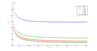
Figure 1 presents the computed values of $\tau_{k}^{*}$ when $p=5$, for different values of $I$. The values of $\tau_{k}^{*}$ are tabulated in Tables 1 and 2 for some selected values of $k$. These experimental results are in agreement with the fact that $\tau_{k}^{*}$ tends to the constant indicated in the right-hand side of (40) as $k$ tends to infinity.

Figure 1: The computed values of $\tau_{k}^{*}$ are plotted against $k$ when $p=5$.

$k$	I = 50	I = 100	I = 160	I = 250	I = 320	I = 400
20	0.6426	0.5913	0.5810	0.5771	0.5760	0.5755
30	0.6401	0.5881	0.5778	0.5739	0.5728	0.5722
40	0.6391	0.5865	0.5762	0.5723	0.5712	0.5706
50	0.6386	0.5856	0.5752	0.5713	0.5703	0.5697
60	0.6384	0.5851	0.5746	0.5707	0.5697	0.5691
70	0.6384	0.5847	0.5742	0.5703	0.5693	0.5687
80	0.6383	0.5844	0.5739	0.5700	0.5689	0.5683

Table 1: The computed values of $\tau_{k}^{*}(\times 10^{-2})$ when $p=5$.

$k$	I = 50	I = 100	I = 160	I = 250	I = 320	I = 400
20	0.1279	0.0826	0.0726	0.0688	0.0677	0.0671
30	0.1279	0.0825	0.0724	0.0686	0.0675	0.0670
40	0.1279	0.0825	0.0724	0.0685	0.0674	0.0669
50	0.1279	0.0825	0.0723	0.0684	0.0674	0.0668
60	0.1279	0.0825	0.0723	0.0684	0.0673	0.0667
70	0.1279	0.0825	0.0723	0.0683	0.0673	0.0667
80	0.1279	0.0825	0.0723	0.0683	0.0673	0.0667

Table 2: The computed values of $\tau_{k}^{*}(\times 10^{-2})$ when $p=7$.

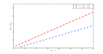
In Figure 2, we show the plot of $\left\|\mathbf{U}_{h,\tau}(t)\right\|_{\infty}$ versus $(T_{h,\tau}-t)$ in log-scale where $T_{h,\tau}$ is given by $T_{h,\tau}=\sum_{k=0}^{K}\lambda^{2k}\tau_{k}^{*}$. The slope of the obtained curves measures the blow-up rate. As expected from (37), these slopes for $p=5$ and $p=7$ are $\frac{1}{4}$ and $\frac{1}{6}$ respectively.

Figure 2: Blow-up rate (in log-scale) when $p=5$ and $p=7$, for $I=400$.

In order to examine the theoretical profile defined in (8), we recall the method of Berger and Kohn [9] to consider the rescaled profile,

$$z\to u^{(k)}\left(z\lambda^{-1}\xi_{k-1}^{+},\tau_{k}^{*}\right),\quad|z|<1,$$ (41)

where $\xi_{q}^{+}=\xi_{q,i_{q}^{+}}$. Using the semilarity variables defined in (4) and (38), we get

$$u^{(k)}(\xi_{k},\tau_{k}^{*})=\lambda^{\frac{2k}{p-1}}(T-t_{k})^{-\frac{1}{p-1}}w\left(\lambda^{k}\frac{\xi_{k}}{\sqrt{T-t_{k}}},s_{k}\right),$$ (42)

where $s_{k}=-\log{(T-t_{k})}$.
We recall from (39) that

$$T-t_{k}\sim\left(\lambda^{2k}M^{1-p}\right)(p-1)^{-1}.$$ (43)

Substituting (43) into (42) yields

$$u^{(k)}(\xi_{k},\tau_{k}^{*})\sim(p-1)^{\frac{1}{p-1}}Mw\left(\sqrt{p-1}M^{\frac{p-1}{2}}\xi_{k},s_{k}\right).$$

From (7), we replace $\xi_{k}$ by $z\lambda^{-1}\xi_{k-1}^{+}$ to obtain

$$u^{(k)}(z\lambda^{-1}\xi_{k-1}^{+},\tau_{k}^{*})\sim(p-1)^{\frac{1}{p-1}}Mf\left(\sqrt{p-1}M^{\frac{p-1}{2}}z\lambda^{-1}\frac{\xi_{k-1}^{+}}{\sqrt{s_{k}}}\right).$$ (44)

Assume that $\frac{\xi_{k-1}^{+}}{\sqrt{s_{k}}}$ tends to $\zeta$. Using the fact that $\alpha M=u^{(k-1)}(\xi_{k-1}^{+},\tau_{k}^{*})$ yields

$$\alpha M=M(p-1)^{\frac{1}{p-1}}f\left(\sqrt{p-1}M^{\frac{p-1}{2}}\zeta\right),$$

or

$$\alpha=(p-1)^{\frac{1}{p-1}}f\left(A\zeta\right),\quad A=\sqrt{p-1}M^{\frac{p-1}{2}}.$$

Using the definition of $f$ in (8), it holds that

$$\alpha=(p-1)^{\frac{1}{p-1}}\left(p-1+\frac{(p-1)^{2}}{4p}|A\zeta|^{2}\right)^{\frac{-1}{p-1}}.\\$$

A straightforward computation gives

$$|A\zeta|^{2}=\frac{4p}{p-1}\left(\alpha^{1-p}-1\right).$$ (45)

Using (45) and (44), we arrive at

$$u^{(k)}(z\lambda^{-1}y_{k-1}^{+},\tau_{k}^{*}) \sim M(p-1)^{\frac{1}{p-1}}f\left(\lambda^{-1}z(A\zeta)\right)^{-\frac{1}{p-1}}$$ (46)

$$\sim M(p-1)^{\frac{1}{p-1}}\left(p-1+\frac{(p-1)^{2}}{4p}\lambda^{-2}z^{2}|A\zeta|^{2}\right)^{-\frac{1}{p-1}}$$

$$\sim M\left(1+\left(\alpha^{1-p}-1\right)\lambda^{-2}z^{2}\right)^{-\frac{1}{p-1}}.$$

Since $\mathbf{U}^{(k)}_{h,\tau}$ converges to $u^{(k)}$ as $h$ goes to zero, it holds that

$$\mathbf{U}^{(k)}_{h,\tau}(z\lambda^{-1}\xi_{k-1}^{+},\tau_{k}^{*})\sim M\left(1+\left(\alpha^{1-p}-1\right)\lambda^{-2}z^{2}\right)^{-\frac{1}{p-1}},\quad|z|<1.$$ (47)

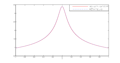
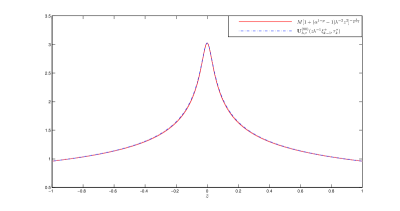
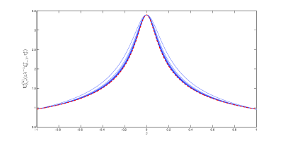
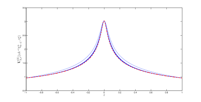
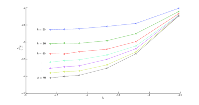
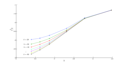
We expect that the left-hand side of (47) tends to the predicted profile as $k$ tends to infinity. Figures 3 and 4 display this relationship after 80 iterations with $I=400$. Figures 5 and 6 illustrate the output of our algorithm using $I=400$ at some selected values of $k$. As $k$ increases these computed profiles converge to the profile shown in Figures 3 and 4 respectively. We give in Tables 3 and 4 the error in $L^{\infty}$-norm between the computed profiles and the predicted profile using various values of $I$ in both cases $p=5$ and $p=7$. The expression of the error is given by

$$e^{(k)}_{h,\tau}=\sup_{-1\leq z\leq 1}\left|\mathbf{U}_{h,\tau}^{(k)}(z\lambda^{-1}\xi_{k-1}^{+},\tau_{k}^{*})-M[1+(\alpha^{1-p}-1)\lambda^{-2}z^{2}]^{-\frac{1}{p-1}}\right|.$$

The graphs of $e^{(k)}_{h,\tau}$ versus $h$ in log-scale are visualized in Figures 7 and 8. We observe in those figures that the error tends to zeros as $h\to 0$. We note that the error $e^{(k)}_{h,\tau}$ includes two sources: the discretization error in using the scheme (17) and the asymptotic error which refers to the behavior of $w(y,s)$ as $s$ tends to infinity.

Figure 3: The computed profile (41) for $k=80$ with $I=400$ and the predicted profile (47) with $p=5$.

Figure 4: The computed profile (41) for $k=80$ with $I=400$ and the predicted profile (47) with $p=7$.

Figure 5: The computed profiles as in (41) for selected values of $k$ with $I=400$ and $p=5$.

Figure 6: The computed profiles as in (41) for selected values of $k$ with $I=400$ and $p=7$.

$k$	I = 50	I = 100	I = 160	I = 250	I = 320	I = 400
10	0.2023	0.1581	0.1501	0.1466	0.1446	0.1432
20	0.1336	0.0858	0.0787	0.0735	0.0722	0.0715
30	0.1213	0.0636	0.0517	0.0480	0.0483	0.0474
40	0.1141	0.0504	0.0404	0.0376	0.0351	0.0354
50	0.1091	0.0444	0.0341	0.0297	0.0289	0.0276
60	0.1076	0.0409	0.0300	0.0249	0.0241	0.0231
70	0.1068	0.0372	0.0255	0.0214	0.0209	0.0202
80	0.1066	0.0354	0.0232	0.0188	0.0182	0.0174

Table 3: Error in $L^{\infty}$-norm between the computed profile and the predicted profile for selected values of $k$ using various values of $I$ with $p=5$.

$k$	I = 50	I = 100	I = 160	I = 250	I = 320	I = 400
10	0.2900	0.1930	0.1205	0.0887	0.0792	0.0730
20	0.2748	0.1757	0.0970	0.0651	0.0556	0.0516
30	0.2711	0.1715	0.0880	0.0545	0.0451	0.0398
40	0.2725	0.1699	0.0843	0.0484	0.0391	0.0337
50	0.2723	0.1696	0.0822	0.0441	0.0351	0.0295
60	0.2706	0.1695	0.0810	0.0421	0.0322	0.0265
70	0.2726	0.1694	0.0803	0.0403	0.0298	0.0240
80	0.2720	0.1694	0.0802	0.0393	0.0285	0.0224

Table 4: Error in $L^{\infty}$-norm between the computed profile and the predicted profile for selected values of $k$ using various values of $I$ with $p=7$.

Figure 7: Error between the computed profiles and the predicted profile in log-scale when $p=5$.

Figure 8: Error between the computed profiles and the predicted profile in log-scale when $p=7$.

5.2 The nonlinear heat equation in case $\beta\neq 0$

5.2.1 A formal calculation

This part gives a formal calculation to obtain the prediction given in (12). This kind of arguments can be found in [9], [40] and [39]. Using similarity variables defined in (4) with $a=0$, we see that $w=w_{0,T}$ satisfies the following equation for all $s\geq-\log{T}$ and $y\in\mathbb{R}^{N}$:

$$w_{s}=\Delta w-\frac{1}{2}y.\nabla w-\frac{w}{p-1}+|w|^{p-1}w+\beta|\nabla w|^{\frac{2p}{p+1}}.$$ (48)

We try to find a solution of (48) in the form $v\left(\frac{y}{\sqrt{s}}\right)$, with

$$v(0)=\kappa,\quad\lim_{|z|\to+\infty}|v(z)|=0.$$

A computation shows that $v$ must satisfy the following equation, for each $s\geq-\log T$ and each $z\in\mathbb{R}^{N}$:

$$-\frac{z.\nabla v(z)}{2s}=\frac{1}{s}\Delta v(z)-\frac{z.\nabla v(z)}{2}-\frac{v(z)}{p-1}+|v(z)|^{p-1}v(z)+\frac{\beta}{s^{\frac{p}{p+1}}}|\nabla v(z)|^{\frac{2p}{p+1}}.$$ (49)

We formally seek regular solutions of (48) in the form

$$V(z)=v_{0}\left(z\right)+\dfrac{1}{s^{\alpha}}R(z,s),$$

where $z=\frac{y}{\sqrt{s}}$, $\alpha>0$ and $\|R\|_{L^{\infty}}\leq C$.
Pugging this ansatz in (49) and making $s\to+\infty$, we obtain the following equation satisfied by $v_{0}$,

$$-\frac{1}{2}zv_{0}^{\prime}(z)-\frac{1}{p-1}v_{0}(z)+v_{0}(z)^{p}=0.$$ (50)

Solving (50) yields

$$v_{0}(z)=\left(p-1+bz^{2}\right)^{-\frac{1}{p-1}},$$ (51)

for some constant $b=b(\beta)\in\mathbb{R}$. We impose $b(\beta)>0$ in order to have a bounded constant solution.

Remark 12.

In the case $\beta=0$, imposing an analyticity condition, Berger and Kohn [9] have formally found $b(0)=\frac{(p-1)^{2}}{4p}$, which is the coefficient of $f$ given in (8). The value of $c_{0}$ was confirmed in several contributions (Filippas and Kohn [22], Herrero and Velázquez [35], Bricmont and Kupiainen [10]). Unfortunately, we were not able to adapt the formal approach of [9] in the case $\beta\neq 0$, so we only have a numerical expression of $\beta$ in Figure 12 below.

5.2.2 Numerical simulations

An important aim in this work is to give a numerical confirmation for the conjectured profile given in (10). Note that we have just given a formal argument in the previous subsection, for the existence of that profile, without, specifying the value of $b(\beta)$. Up to our knowledge, there is neither a rigorous proof nor a numerical confirmation for (10), and our paper is the first to exhibit such a solution numerically. More importantly, thanks to our computations, we are able to find a numerical approximation of $b(\beta)$ in the formula of $\bar{f}_{\beta}$ in (11) from our computations.

If we make the same analysis to check that the numerical profile fits with the conjecture theoretical profile (10) as the above analysis when $\beta=0$, then the same result holds in this case, namely

$$u^{(k)}(z\lambda^{-1}\xi_{k-1}^{+},\tau_{k}^{*})\sim M\left(1+\left(\alpha^{1-p}-1\right)\lambda^{-2}z^{2}\right)^{-\frac{1}{p-1}},\quad-1<z<1.$$ (52)

Figures 9 and 10 show the graphs of the computed profile $\mathbf{U_{h,\tau}^{(80)}}(z\lambda^{-1}\xi_{k-1}^{+},\tau_{k}^{*})$ and the predicted profile given in the right hand side of (52), for computations using $I=320$, $\beta=1$, $p=5$ and $p=7$.

Figure 9: The computed and the predicted profiles in (52), for computations using $I=320$, $\beta=1$ and $p=5$.

Figure 10: The computed and the predicted profiles in (52), for computations using $I=320$, $\beta=1$ and $p=7$.

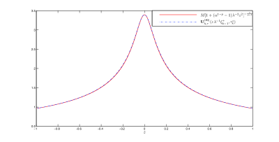
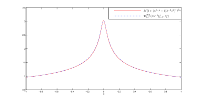
In order to compute the value of $b(\beta)$ from the simulations, we use the relation (42) with $\xi_{k}=z\lambda^{-1}\xi_{k-1}^{+}$, we get

$$u^{(k)}(z\lambda^{-1}\xi_{k-1}^{+},\tau_{k}^{*})=\lambda^{\frac{2k}{p-1}}(T-t_{k})^{-\frac{1}{p-1}}w\left(\lambda^{k}\frac{z\lambda^{-1}\xi_{k-1}^{+}}{\sqrt{T-t_{k}}},s_{k}\right).$$ (53)

We recall from (11) that the predicted profile $\bar{f}_{\beta}$ is given by

$$\bar{f}_{\beta}(z)=\kappa\left(1+\frac{b(\beta)}{p-1}z^{2}\right)^{-\frac{1}{p-1}},\quad z=\frac{x}{\sqrt{(T-t)|\log(T-t)|}},\quad\kappa=(p-1)^{-\frac{1}{p-1}},$$ (54)

and that

$$\sup_{|z|<K}\left|w(y,s)-\bar{f}_{\beta}(z)\right|\to 0\quad\text{as }s\to\infty\quad\text{with }z=\frac{y}{\sqrt{s}}.$$ (55)

From (55), (54) and (53), ignoring the error of asymptotic behavior as $s$ goes to infinity, we obtain

$$u^{(k)}(z\lambda^{-1}\xi_{k-1}^{+},\tau_{k}^{*}) =\lambda^{\frac{2k}{p-1}}(T-t_{k})^{-\frac{1}{p-1}}f\left(\lambda^{k}\frac{z\lambda^{-1}\xi_{k-1}^{+}}{\sqrt{T-t_{k}}}\times\frac{1}{\sqrt{s_{k}}}\right)$$

$$=\lambda^{\frac{2k}{p-1}}(T-t_{k})^{\frac{-1}{p-1}}\kappa\left(1+\frac{b(\beta)}{p-1}\frac{\lambda^{2k}z^{2}\lambda^{-2}(\xi_{k-1}^{+})^{2}}{T-t_{k}}\frac{1}{s_{k}}\right)^{-\frac{1}{p-1}}.$$

After some straightforward calculations, we arrive at

$$b(\beta)=\frac{s_{k}}{(\xi_{k-1}^{+})^{2}}\left[\frac{\kappa\lambda^{2k}(p-1)[u^{(k)}(z\lambda^{-1}\xi_{k-1}^{+},\tau_{k}^{*})]^{1-p}-(p-1)(T-t_{k})}{\lambda^{2k-2}z^{2}}\right].$$

Setting $z=\lambda$ and taking the limit of the above equation as $k$ goes to infinity, we get

$$b(\beta)=\lim_{k\to+\infty}\frac{s_{k}}{(\xi_{k-1}^{+})^{2}}\zeta_{k},$$

where

$$\zeta_{k}=(p-1)\left(\kappa[u^{(k)}(\xi_{k-1}^{+},\tau_{k}^{*})]^{1-p}-\lambda^{-2k}(T-t_{k})\right).$$

Using (39) and (52), we see that $\zeta_{k}$ approaches a limit given by

$$\lim_{k\to+\infty}\zeta_{k}=M^{1-p}\left[(p-1)\kappa\alpha^{1-p}-1\right].$$

This implies that the ratio $\frac{s_{k}}{(\xi_{k-1}^{+})^{2}}$ should approach a constant as $k$ tends to infinity. This is presented in Figure 11.

Figure 11: The graph of $\frac{s_{k}}{(\xi_{k-1}^{+})^{2}}$ versus $k$, for computations using $I=320$, $p=5$ and $\beta=0$.

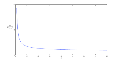
We remark that the computations of $s_{k}$ and $\zeta_{k}$ do not depend on $\beta$. Moreover, we know that the value of $b(0)$ is $\frac{(p-1)^{2}}{4p}$. In particular, we compute the value of $b(\beta)$ by

$$b(\beta)=\frac{C_{K}}{\left[\xi_{K-1}^{+}(\beta)\right]^{2}},$$

where $C_{K}=b(0)\left[\xi_{K-1}^{+}(0)\right]^{2}$ for $K$ large.

Figure 12: The computed values of $b(\beta)$. (Left) $p=5$. (Right) $p=7$.

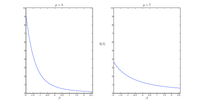
Consequently, we have just given a numerical evidence for the following conjecture:

Conjecture 6.

Equation (1) has a solution $u(x,t)$ which blows up in finite time $T$ with

$$\sup_{|z|<K}|(T-t)^{1/(p-1)}u(x,t)-\bar{f_{\beta}}(z)|\to 0,\quad\text{as}\quad t\to T,$$ (56)

where $K>0,z=\frac{x}{\sqrt{(T-t)|\log(T-t)|}}$ and

$$\bar{f_{\beta}}(z)=\left(p-1+b(\beta)|z|^{2}\right)^{-\frac{1}{p-1}},\quad\text{with}\quad b(0)=\frac{(p-1)^{2}}{4p},$$

and $b(\beta)$ is represented in Figure 12, for $p=5$ and $p=7$.

While remarking numerical simulation for equation (1) with $\beta\neq 0$, we could never obtain the self-similar behavior (9) rigorously proved in [49]. On the contrary, we could exhibit the behavior (56), at the heart of our conjecture. In our opinion, this is probably due to the fact that the behavior (9) is unstable, unlike the behavior (56), which we suspect to be stable with respect to perturbations in initial data.

5.3 The complex Ginzburg-Landau equation

We recall that $e^{\imath\theta}\tilde{f}_{\delta,\gamma}$ is an asymptotic profile of the solution of (2) where $\theta\in\mathbb{R}$ and $\tilde{f}_{\delta,\gamma}$ is given in (15), namely

$$\tilde{f}_{\delta,\gamma}=\left(p-1+b(\delta,\gamma)|z|^{2}\right)^{-\frac{1+\imath\delta}{p-1}},\quad b(\delta,\gamma)=\frac{(p-1)^{2}}{4(p-\delta^{2}-\gamma\delta-\gamma\delta p)}>0.$$ (57)

Using the same analysis as Section 5.1 resulting (46), we have for $|z|<1$,

$$u^{(k)}(z\lambda^{-1}y_{k-1}^{+},\tau_{k}^{*})\sim M^{1+\imath\delta}\lambda^{-\frac{2\imath k\delta}{p-1}}(p-1)^{\frac{\imath\delta}{p-1}}e^{\imath\theta}\left(1+(\alpha^{1-p}-1)\lambda^{-2}z^{2}\right)^{-\frac{1+\imath\delta}{p-1}}.$$ (58)

Remark 13.

We remark that the rescaled profile (58) is obtained under the assumption $p-\delta^{2}-\gamma\delta(p+1)>0$. If this condition is not satisfied, the question is open.

Remark 14.

If we take the modulus and the phase of both sides in (58), then we get

$$\left|u^{(k)}\right|(z\lambda^{-1}y_{k-1}^{+},\tau_{k}^{*})\sim M(1+(\alpha^{1-p}-1)\lambda^{-2}z^{2})^{-\frac{1}{p-1}},\quad|z|<1,$$ (59)

$$phase\left[u^{(k)}\right](z\lambda^{-1}y_{k-1}^{+},\tau_{k}^{*}) \sim\theta+\frac{\delta}{p-1}\left(\ln M+\ln(p-1)-2k\ln\alpha\right)$$

$$-\frac{\delta}{p-1}\ln\left(1+(\alpha^{1-p}-1)\lambda^{-2}z^{2}\right),\quad|z|<1.$$ (60)

The right hand side of (59) is the same as in (46).

5.3.1 Experiments with $p-\delta^{2}-\gamma\delta(p+1)>0$.

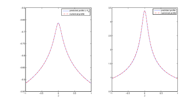
We first make an experiment with $\gamma=0,\,\delta=0.2,\,p=5$ and the initial grid with $I=320$. The numerical result displayed in Figure 13 is in agreement with the expectation obtained in (59) and (60). Both the numerical modulus and phase coincide with the predicted profile given in (59) and (60) within plotting resolution.

Figure 13: Comparing the numerical profile with the predicted profile given in (59) and (60) after 80 iterative steps ($\gamma=0,\delta=0.2,p=5,I=320$). (Left) $phase\left[u^{(k)}\right](z\lambda^{-1}y^{+}_{k-1},\tau_{k}^{*})$. (Right) $\left|u^{(k)}\right|(z\lambda^{-1}y^{+}_{k-1},\tau_{k}^{*})$.

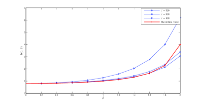
An experiment with $\gamma=0,\,p=5$ and various values of $\delta$ are performed on three grids with $I=100,200,320$. The purpose is to confirm the theoretical profile $\tilde{f}_{\delta,\gamma}$ given in (57). More precisely, we would like to calculate values of $b(\delta,0)$ from our numerical simulation. We recall that the theoretical value of $b(\delta,0)$ is equal to $\frac{(p-1)^{2}}{p-\delta^{2}}$. In Figure 14, we have the computed values of $b(\delta,0)$ on various initial grids $I$. Note that these computed values tend to the predicted ones as $I$ increases. However, as $\delta$ approaches $\sqrt{p}$ ($\sqrt{5}$ in Figure 14), $b$ becomes singular, and that is the reason why the coincidence between the numerical and theoretical values becomes less clear.

Figure 14: The computed values of $b(\delta,0)$ for various initial grids when $p=5$.

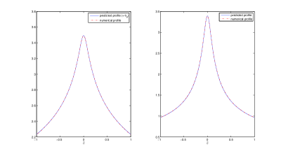
A further experiment with $\gamma=1,\,\delta=1$ is shown in Figure 15. These calculations show the relationship we obtained in (59) and (60). Both the numerical phase and modulus coincide with the predicted ones given in (59) and (60) within plotting resolution.

Figure 15: Comparing the numerical profile with the predicted profile given in (59) and (60) after 80 iterative steps ($\gamma=1,\delta=1,p=5,I=320$). (Left) $phase\left[u^{(k)}\right](z\lambda^{-1}y^{+}_{k-1},\tau_{k}^{*})$. (Right) $\left|u^{(k)}\right|(z\lambda^{-1}y^{+}_{k-1},\tau_{k}^{*})$.

5.3.2 Experiments with $p-\delta^{2}-\gamma\delta(p+1)<0$.

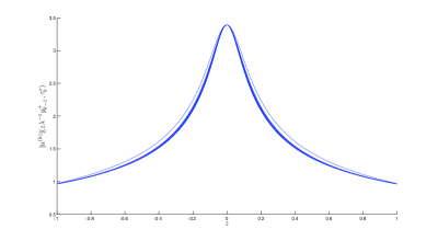
In this section, we make some experiments with $\gamma=0$ and $\delta>\sqrt{p}=\sqrt{5}$. For $\delta$ large enough, there is no blow-up phenomenon (for example with $\delta=3$). With $\delta$ near $\sqrt{p}$, we made two simulations with $\delta=\sqrt{p}+0.1$ and $\delta=\sqrt{p}+0.5$, then the blow-up phenomenon still occurs. Figure 16 displays the modulus of $u^{(k)}(z\lambda^{-1}y_{k-1}^{+},\tau_{k}^{*})$ at some selected values of $k$, for computations using the initial grid $I=320$. It shows the rescaled profile $z\mapsto\left|u^{(k)}\right|(z\lambda^{-1}y_{k-1}^{+},\tau_{k}^{*})$. We can see that these rescaled profiles converge as $k$ increases.

Figure 16: The numerical values of $u^{(k)}(z\lambda^{-1}y_{k-1}^{+},\tau_{k}^{*})$ at some selected values of $k$, for computation using the initial grid $I=320$ with $p=5$. (Above) $\gamma=0,\delta=\sqrt{p}+0.1$. (Below) $\gamma=0,\delta=\sqrt{p}+0.5$.

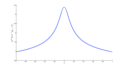
Consequently, if $p-\delta^{2}-\gamma\delta-\gamma\delta p<0$, the blow-up phenomenon may occur and there may exist a blow-up profile. So far, we have no answer for this case. We wonder whether its solution behaves as the solution in the case $p-\delta^{2}-\gamma\delta-\gamma\delta p>0$ with a different function of $b(\delta,\gamma)$ in formula of $\tilde{f}_{\delta,\gamma}$ given in (57).

Appendix A A regularity result for equation (1)

We claim the following:

Proposition A.1 (Parabolic regularity).

Consider $u$ solution of

$$\left\{\begin{array}[]{lll}u_{t}&=u_{xx}+|u|^{p-1}u+\beta|u_{x}|^{q},&\text{in}\quad\Omega\times(0,T),\\ u(x,t)&=0&\text{on}\quad\partial\Omega\times[0,T),\\ u(x,0)&=u_{0}(x),&\text{on}\quad\bar{\Omega}.\end{array}\right.$$ (61)

where $u(t):x\in\Omega\mapsto\mathbb{R}$ with $\Omega$ is an interval in $\mathbb{R}$, $p,q>1$ and $\beta\in\mathbb{R}$.
Assume that $\|u_{0}\|_{\mathcal{C}^{2}(\bar{\Omega})}\leq C_{0}$ and $\|u\|_{\mathcal{C}(\bar{\Omega}\times[0,T_{0}])}+\|u_{x}\|_{\mathcal{C}(\bar{\Omega}\times[0,T_{0}])}\leq C_{u}$ with $T_{0}<T$ ($T$ is the existence time of the maximal solution). Then for all $t\in[0,T_{0}]$,
$i)\|u_{xx}(t)\|_{L^{\infty}(\bar{\Omega})}+\|u_{t}(t)\|_{L^{\infty}(\bar{\Omega})}\leq C$ for some $C=C(C_{0},C_{u},T_{0},p,q,\beta)$.
Assume in addition, $\|u_{0}\|_{\mathcal{C}^{4}(\bar{\Omega})}\leq C_{0}$ and $p,q\geq 2$. Then for all $t\in[0,T_{0}]$,
$ii)\quad\|u_{xxx}(t)\|_{L^{\infty}(\bar{\Omega})}+\|u_{xxxx}(t)\|_{L^{\infty}(\bar{\Omega})}+\|u_{tt}(t)\|_{L^{\infty}(\bar{\Omega})}\leq C$ for some $C=C(C_{0},C_{u},T_{0},p,q,\beta)$.

Remark 15.

Chipot and Weissler showed in [14] (see Proposition 2.2) that for $s\in\mathbb{R}$ sufficient large and $u_{0}\in W_{0}^{1,s}(\Omega)$, then $u$, a solution of (61), satisfies that

$$\|u(t)\|_{L^{\infty}}\quad\text{and}\quad\|u_{x}(t)\|_{L^{\infty}}\quad\text{are bounded for any inteval $[0,T_{0}]$ with $T_{0}<T$}.$$

Proof of Proposition A.1.

In what follows, we write $\|\cdot\|_{\infty}=\|\cdot\|_{L^{\infty}(\bar{\Omega})}$ for simplicity and denote by $C_{1},C_{2},\dots$ constants depending only on $C_{0},C_{u},T_{0},p,q$ and $\beta$.

$i)$ We see from (61) that $\|u_{t}(t)\|_{\infty}$ is bounded on $[0,T_{0}]$ if $\|u_{xx}(t)\|_{\infty}$ is bounded on $[0,T_{0}]$. Let us consider $h=u_{xx}$, then $h$ satisfies

$$h_{t}=h_{xx}+\partial_{x}\left(p|u|^{p-1}u_{x}+q\beta|u_{x}|^{q-2}u_{x}h\right).$$ (62)

An integral form of the solution of equation (62) is

$$h(t)=e^{t\Delta}h(0)+\int_{0}^{t}e^{(t-s)\Delta}\partial_{x}\left(p|u(s)|^{p-1}u_{x}(s)+q\beta|u_{x}(s)|^{q-2}u_{x}(s)h(s)\right)ds,$$ (63)

where $e^{t\Delta}$ denotes the heat semigroup on $\Omega$ with Dirichlet boundary condition.
Recall that for all $\varphi\in L^{\infty}$,

$$\|e^{t\Delta}\varphi\|_{\infty}\leq\|\varphi\|_{\infty}\quad\text{and}\quad\|e^{t\Delta}\nabla\varphi\|_{\infty}\leq\frac{C^{\prime}}{\sqrt{t}}\|\varphi\|_{\infty}.$$ (64)

Since $u_{0}\in\mathcal{C}^{2}$ and $\|u(t)\|_{\infty},\|u_{x}(t)\|_{\infty}$ are bounded for all $t\in[0,T_{0}]$, then we have by (64) and (63) that

$$\|h(t)\|_{\infty}\leq C_{1}+C_{1}\int_{0}^{t}\frac{\|h(s)\|_{\infty}}{\sqrt{t-s}}ds,\quad\forall t\in[0,T_{0}].$$

Using a Growall’s argument, we have

$$\|h(t)\|_{\infty}\leq 2C_{1}e^{C_{1}\sqrt{T_{0}}},\quad\forall t\in[0,T_{0}].$$

Therefore, $\|u_{xx}(t)\|_{\infty}$ is bounded for all $t\in[0,T_{0}]$ which concludes the proof of $i)$.

$ii)$ We assume additionally in what follows that $p,q\geq 2$, $\|u_{0}\|_{\mathcal{C}^{4}(\bar{\Omega})}\leq C_{0}$. Consider $v=u_{xxx}$, let us show that $\|v(t)\|_{\infty}$ is bounded for all $t\in[0,T_{0}]$. From (61) we see that $v$ satisfies the following equation

$$v_{t}=v_{xx}+p|u|^{p-1}v+\beta q\partial_{x}(|u_{x}|^{q-2}u_{x}v)+\phi+\partial_{x}\psi,$$ (65)

where

$$\phi =p(p-1)|u|^{p-3}uu_{x}u_{xx},\psi =p(p-1)|u|^{p-3}u(u_{x})^{2}+\beta q(q-1)|u_{x}|^{q-2}(u_{xx})^{2}.$$

We now use an integral formulation of (65) to write

$$v(t)=e^{t\Delta}v(0) +p\int_{0}^{t}e^{(t-s)\Delta}|u(s)|^{p-1}v(s)ds$$

$$+\beta q\int_{0}^{t}e^{(t-s)\Delta}\partial_{x}(|u_{x}(s)|^{q-2}u_{x}(s)v(s))ds$$

$$+\int_{0}^{t}e^{(t-s)\Delta}\phi(s)ds+\int_{0}^{t}e^{(t-s)\Delta}\partial_{x}\psi(s)ds.$$

From $(i)$ and the hypothesis on $u_{0}\in\mathcal{C}^{4}$, we see that for all $t\in[0,T_{0}]$,

$$\|v(0)\|_{\infty}+\|u(t)\|_{\infty}^{p-1}+\|u_{x}(t)\|_{\infty}^{q-1}+\|\phi(t)\|_{\infty}+\|\psi(t)\|_{\infty}\leq C_{2}.$$

Hence, the use of (64) yields

$$\|v(t)\|_{\infty}\leq C_{2}+C_{2}\int_{0}^{t}\left(1+\frac{1}{\sqrt{t-s}}\right)\|v(s)\|_{\infty}ds\leq 2C_{2}e^{C_{2}(T_{0}+2\sqrt{T_{0}})},\quad\forall t\in[0,T_{0}],$$

which follows that $\|u_{xxx}(t)\|_{\infty}$ is bounded on $[0,T_{0}]$.

We now bound $\|u_{tt}(t)\|_{\infty}$ on $[0,T_{0}]$. Consider $\theta=u_{tt}$, by (61), we see that $\theta$ satisfies

$$\theta_{t}=\theta_{xx}+\eta\theta+\beta q\partial_{x}\left(|u_{x}|^{q-2}u_{x}\theta\right)+\gamma,$$ (66)

where

$$\eta =p|u|^{p-1}-\beta q(q-1)|u_{x}|^{q-2}u_{xx},$$

$$\gamma =p(p-1)|u|^{p-3}u(u_{t})^{2}+\beta q(q-1)|u_{x}|^{q-2}\left(u_{xxx}+p|u|^{p-1}u_{x}+\beta q|u_{x}|^{q-2}u_{x}u_{xx}\right)^{2}.$$

An integral form of the solution of equation (66) is

$$\theta(t)=e^{t\Delta}\theta(0) +\int_{0}^{t}e^{(t-s)\Delta}\eta(s)\theta(s)ds$$

$$+\beta q\int_{0}^{t}e^{(t-s)\Delta}\partial_{x}\left(|u_{x}(s)|^{q-2}u_{x}(s)\theta(s)\right)ds+\int_{0}^{t}e^{(t-s)\Delta}\gamma(s)ds.$$

Since $u_{0}\in\mathcal{C}^{4}$, then $\|\theta(0)\|_{\infty}=\|u_{tt}(0)\|_{\infty}$ is bounded. Using the fact that $\|u_{xxx}(t)\|_{\infty}$ is bounded on $[0,T_{0}]$ and $(i)$, we have by (64) that

$$\|\theta(t)\|_{\infty}\leq C_{3}+C_{3}\int_{0}^{t}\left(1+\frac{1}{\sqrt{t-s}}\right)\|\theta(s)\|_{\infty}ds\leq 2C_{3}e^{C_{3}(T_{0}+2\sqrt{T_{0}})},\quad\forall t\in[0,T_{0}].$$

Since $\|u_{tt}(t)\|_{L^{\infty}}$ is bounded on $[0,T_{0}]$, we have from (61) that $\|u_{xxxx}(t)\|_{L^{\infty}}$ is also bounded on $[0,T_{0}]$. This completes the proof of Proposition A.1. ∎

References

-
Abia et al. [1996]
Abia, L. M., López-Marcos, J. C., Martínez, J., 1996. Blow-up for
semidiscretizations of reaction-diffusion equations. Appl. Numer. Math.
20 (1-2), 145–156, workshop on the method of lines for time-dependent
problems (Lexington, KY, 1995).
URL http://dx.doi.org/10.1016/0168-9274(95)00122-0 -
Abia et al. [1998]
Abia, L. M., López-Marcos, J. C., Martínez, J., 1998. On the blow-up
time convergence of semidiscretizations of reaction-diffusion equations.
Appl. Numer. Math. 26 (4), 399–414.
URL http://dx.doi.org/10.1016/S0168-9274(97)00105-0 -
Abia et al. [2001]
Abia, L. M., López-Marcos, J. C., Martínez, J., 2001. The Euler
method in the numerical integration of reaction-diffusion problems with
blow-up. Appl. Numer. Math. 38 (3), 287–313.
URL http://dx.doi.org/10.1016/S0168-9274(01)00035-6 -
Acosta et al. [2002a]
Acosta, G., Durán, R. G., Rossi, J. D., 2002a. An adaptive
time step procedure for a parabolic problem with blow-up. Computing 68 (4),
343–373.
URL http://dx.doi.org/10.1007/s00607-002-1449-x -
Acosta et al. [2002b]
Acosta, G., Fernández Bonder, J., Groisman, P., Rossi, J. D.,
2002b. Numerical approximation of a parabolic problem with a
nonlinear boundary condition in several space dimensions. Discrete Contin.
Dyn. Syst. Ser. B 2 (2), 279–294.
URL http://dx.doi.org/10.3934/dcdsb.2002.2.279 -
Assalé et al. [2008]
Assalé, L. A., K., B. T., Diabate, N., 2008. Numerical blow-up time for a
semilinear parabolic equation with nonlinear boundary conditions. Journal of
Applied Mathematics 2008, Article ID 753518, 29 p.–Article ID 753518, 29 p.
URL http://eudml.org/doc/45748 - Ball [1977] Ball, J. M., 1977. Remarks on blow-up and nonexistence theorems for nonlinear evolution equations. Quart. J. Math. Oxford Ser. (2) 28 (112), 473–486.
Baruch et al. [2010]
Baruch, G., Fibich, G., Gavish, N., 2010. Singular standing-ring solutions of
nonlinear partial differential equations. Phys. D 239 (20-22), 1968–1983.
URL http://dx.doi.org/10.1016/j.physd.2010.07.009 -
Berger and Kohn [1988]
Berger, M., Kohn, R. V., 1988. A rescaling algorithm for the numerical
calculation of blowing-up solutions. Comm. Pure Appl. Math. 41 (6), 841–863.
URL http://dx.doi.org/10.1002/cpa.3160410606 -
Bricmont and Kupiainen [1994]
Bricmont, J., Kupiainen, A., 1994. Universality in blow-up for nonlinear heat
equations. Nonlinearity 7 (2), 539–575.
URL http://stacks.iop.org/0951-7715/7/539 -
Cazenave et al. [2013]
Cazenave, T., Dickstein, F., Weissler, F., 2013. Finite-time blowup for a
complex ginzburg–landau equation. SIAM Journal on Mathematical Analysis
45 (1), 244–266.
URL http://epubs.siam.org/doi/abs/10.1137/120878690 - Chen [1986] Chen, Y. G., 1986. Asymptotic behaviours of blowing-up solutions for finite difference analogue of . J. Fac. Sci. Univ. Tokyo Sect. IA Math. 33 (3), 541–574.
- Chen [1992] Chen, Y. G., 1992. Blow-up solutions to a finite difference analogue of in -dimensional balls. Hokkaido Math. J. 21 (3), 447–474.
Chipot and Weissler [1989]
Chipot, M., Weissler, F. B., 1989. Some blowup results for a nonlinear
parabolic equation with a gradient term. SIAM J. Math. Anal. 20 (4),
886–907.
URL http://dx.doi.org/10.1137/0520060 -
Duran et al. [1998]
Duran, R. G., Etcheverry, J. I., Rossi, J. D., 1998. Numerical approximation of
a parabolic problem with a nonlinear boundary condition. Discrete Contin.
Dynam. Systems 4 (3), 497–506.
URL http://dx.doi.org/10.3934/dcds.1998.4.497 - Ebde and Zaag [2011] Ebde, M. A., Zaag, H., 2011. Construction and stability of a blow up solution for a nonlinear heat equation with a gradient term. SMA J. (55), 5–21.
Fermanian Kammerer et al. [2000]
Fermanian Kammerer, C., Merle, F., Zaag, H., 2000. Stability of the blow-up
profile of non-linear heat equations from the dynamical system point of view.
Math. Ann. 317 (2), 347–387.
URL http://dx.doi.org/10.1007/s002080000096 -
Fermanian Kammerer and Zaag [2000]
Fermanian Kammerer, C., Zaag, H., 2000. Boundedness up to blow-up of the
difference between two solutions to a semilinear heat equation. Nonlinearity
13 (4), 1189–1216.
URL http://dx.doi.org/10.1088/0951-7715/13/4/311 -
Fernández Bonder et al. [2002]
Fernández Bonder, J., Groisman, P., Rossi, J. D., 2002. On numerical
blow-up sets. Proc. Amer. Math. Soc. 130 (7), 2049–2055.
URL http://dx.doi.org/10.1090/S0002-9939-02-06350-5 -
Ferreira et al. [2002]
Ferreira, R., Groisman, P., Rossi, J. D., 2002. Numerical blow-up for a
nonlinear problem with a nonlinear boundary condition. Math. Models Methods
Appl. Sci. 12 (4), 461–483.
URL http://dx.doi.org/10.1142/S021820250200174X -
Ferreira et al. [2004]
Ferreira, R., Groisman, P., Rossi, J. D., 2004. Numerical blow-up for the
porous medium equation with a source. Numer. Methods Partial Differential
Equations 20 (4), 552–575.
URL http://dx.doi.org/10.1002/num.10103 -
Filippas and Kohn [1992]
Filippas, S., Kohn, R. V., 1992. Refined asymptotics for the blowup of
. Comm. Pure Appl. Math. 45 (7), 821–869.
URL http://dx.doi.org/10.1002/cpa.3160450703 - Filippas and Liu [1993] Filippas, S., Liu, W. X., 1993. On the blowup of multidimensional semilinear heat equations. Ann. Inst. H. Poincaré Anal. Non Linéaire 10 (3), 313–344.
- Friedman [1965] Friedman, A., 1965. Remarks on nonlinear parabolic equations. In: Proc. Sympos. Appl. Math., Vol. XVII. Amer. Math. Soc., Providence, R.I., pp. 3–23.
- Fujita [1966] Fujita, H., 1966. On the blowing up of solutions of the Cauchy problem for . J. Fac. Sci. Univ. Tokyo Sect. I 13, 109–124 (1966).
- Galaktionov and Posashkov [1985] Galaktionov, V. A., Posashkov, S. A., 1985. The equation . Localization, asymptotic behavior of unbounded solutions. Akad. Nauk SSSR Inst. Prikl. Mat. Preprint (97), 30.
- Galaktionov and Posashkov [1986] Galaktionov, V. A., Posashkov, S. A., 1986. Asymptotics of the process of nonlinear heat conduction with absorption in the case of a critical value of the parameter. Akad. Nauk SSSR Inst. Prikl. Mat. Preprint (71), 25.
Giga and Kohn [1985]
Giga, Y., Kohn, R. V., 1985. Asymptotically self-similar blow-up of semilinear
heat equations. Comm. Pure Appl. Math. 38 (3), 297–319.
URL http://dx.doi.org/10.1002/cpa.3160380304 -
Giga and Kohn [1987]
Giga, Y., Kohn, R. V., 1987. Characterizing blowup using similarity variables.
Indiana Univ. Math. J. 36 (1), 1–40.
URL http://dx.doi.org/10.1512/iumj.1987.36.36001 -
Giga and Kohn [1989]
Giga, Y., Kohn, R. V., 1989. Nondegeneracy of blowup for semilinear heat
equations. Comm. Pure Appl. Math. 42 (6), 845–884.
URL http://dx.doi.org/10.1002/cpa.3160420607 -
Groisman [2006]
Groisman, P., 2006. Totally discrete explicit and semi-implicit Euler methods
for a blow-up problem in several space dimensions. Computing 76 (3-4),
325–352.
URL http://dx.doi.org/10.1007/s00607-005-0136-0 -
Groisman and Rossi [2001]
Groisman, P., Rossi, J. D., 2001. Asymptotic behaviour for a numerical
approximation of a parabolic problem with blowing up solutions. J. Comput.
Appl. Math. 135 (1), 135–155.
URL http://dx.doi.org/10.1016/S0377-0427(00)00571-9 - Herrero and Velázquez [1992a] Herrero, M. A., Velázquez, J. J. L., 1992a. Comportement générique au voisinage d’un point d’explosion pour des solutions d’équations paraboliques unidimensionnelles. C. R. Acad. Sci. Paris Sér. I Math. 314 (3), 201–203.
Herrero and Velázquez [1992b]
Herrero, M. A., Velázquez, J. J. L., 1992b. Generic behaviour
of one-dimensional blow up patterns. Ann. Scuola Norm. Sup. Pisa Cl. Sci. (4)
19 (3), 381–450.
URL http://www.numdam.org/item?id=ASNSP_1992_4_19_3_381_0 - Herrero and Velázquez [1993] Herrero, M. A., Velázquez, J. J. L., 1993. Blow-up behaviour of one-dimensional semilinear parabolic equations. Ann. Inst. H. Poincaré Anal. Non Linéaire 10 (2), 131–189.
Hirota and Ozawa [2006]
Hirota, C., Ozawa, K., 2006. Numerical method of estimating the blow-up time
and rate of the solution of ordinary differential equations—an application
to the blow-up problems of partial differential equations. J. Comput. Appl.
Math. 193 (2), 614–637.
URL http://dx.doi.org/10.1016/j.cam.2005.04.069 -
Hocking et al. [1972]
Hocking, L. M., Stewartson, K., Stuart, J. T., Brown, S. N., 1 1972. A
nonlinear instability burst in plane parallel flow. Journal of Fluid
Mechanics 51, 705–735.
URL http://journals.cambridge.org/article_S0022112072001326 - Levine [1973] Levine, H. A., 1973. Some nonexistence and instability theorems for solutions of formally parabolic equations of the form . Arch. Rational Mech. Anal. 51, 371–386.
Masmoudi and Zaag [2008]
Masmoudi, N., Zaag, H., 2008. Blow-up profile for the complex
Ginzburg-Landau equation. J. Funct. Anal. 255 (7), 1613–1666.
URL http://dx.doi.org/10.1016/j.jfa.2008.03.008 -
Merle and Zaag [1997]
Merle, F., Zaag, H., 1997. Stability of the blow-up profile for equations of
the type . Duke Math. J. 86 (1),
143–195.
URL http://dx.doi.org/10.1215/S0012-7094-97-08605-1 -
Merle and Zaag [1998a]
Merle, F., Zaag, H., 1998a. Optimal estimates for blowup rate and
behavior for nonlinear heat equations. Comm. Pure Appl. Math. 51 (2),
139–196.
URL http://dx.doi.org/10.1002/(SICI)1097-0312(199802) -
Merle and Zaag [1998b]
Merle, F., Zaag, H., 1998b. Refined uniform estimates at blow-up
and applications for nonlinear heat equations. Geom. Funct. Anal. 8 (6),
1043–1085.
URL http://dx.doi.org/10.1007/s000390050123 - Nakagawa [1975/76] Nakagawa, T., 1975/76. Blowing up of a finite difference solution to . Appl. Math. Optim. 2 (4), 337–350.
- Nakagawa and Ushijima [1977] Nakagawa, T., Ushijima, T., 1977. Finite element analysis of the semi-linear heat equation of blow-up type. in Topics in Numerical Analysis, J. J. H. Miller, ed., Academic Press.
- N’gohisse and Boni [2011] N’gohisse, F. K., Boni, T. K., 2011. Numerical blow-up for a nonlinear heat equation. Acta Math. Sin. (Engl. Ser.) 27 (5), 845–862.
Philippe [1996]
Philippe, S., 1996. Finite time blow-up for a non-linear parabolic equation
with a gradient term and applications. Mathematical Methods in the Applied
Sciences 19 (16), 1317–1333.
URL http://dx.doi.org/10.1002/(SICI)1099-1476 -
Popp et al. [1998]
Popp, S., Stiller, O., Kuznetsov, E., Kramer, L., 1998. The cubic complex
ginzburg-landau equation for a backward bifurcation. Physica D: Nonlinear
Phenomena 114 (1-2), 81 – 107.
URL http://www.sciencedirect.com/science/article/pii/S016727899700170X - Quittner and Souplet [2007] Quittner, P., Souplet, P., 2007. Superlinear parabolic problems. Birkhäuser Advanced Texts: Basler Lehrbücher. [Birkhäuser Advanced Texts: Basel Textbooks]. Birkhäuser Verlag, Basel, blow-up, global existence and steady states.
Souplet et al. [1996]
Souplet, P., Tayachi, S., Weissler, F. B., 1996. Exact self-similar blow-up of
solutions of a semilinear parabolic equation with a nonlinear gradient term.
Indiana Univ. Math. J. 45 (3), 655–682.
URL http://dx.doi.org/10.1512/iumj.1996.45.1197 -
Ushijima [2000]
Ushijima, T. K., 2000. On the approximation of blow-up time for solutions of
nonlinear parabolic equations. Publ. Res. Inst. Math. Sci. 36 (5), 613–640.
URL http://dx.doi.org/10.2977/prims/1195142812 -
Velázquez [1992]
Velázquez, J. J. L., 1992. Higher-dimensional blow up for semilinear
parabolic equations. Comm. Partial Differential Equations 17 (9-10),
1567–1596.
URL http://dx.doi.org/10.1080/03605309208820896 -
Velázquez [1993]
Velázquez, J. J. L., 1993. Classification of singularities for blowing up
solutions in higher dimensions. Trans. Amer. Math. Soc. 338 (1), 441–464.
URL http://dx.doi.org/10.2307/2154464 -
Zaag [1998]
Zaag, H., 1998. Blow-up results for vector-valued nonlinear heat equations with
no gradient structure. Ann. Inst. H. Poincaré Anal. Non Linéaire
15 (5), 581–622.
URL http://dx.doi.org/10.1016/S0294-1449(98)80002-4