On the Configuration LP for Maximum Budgeted Allocation

Abstract

We study the Maximum Budgeted Allocation problem , i.e.,  the problem of selling a set of $m$ indivisible goods to $n$ players, each with a separate budget, such that we maximize the collected revenue. Since the natural assignment LP is known to have an integrality gap of $\frac{3}{4}$, which matches the best known approximation algorithms, our main focus is to improve our understanding of the stronger configuration LP relaxation. In this direction, we prove that the integrality gap of the configuration LP is strictly better than $\frac{3}{4}$, and provide corresponding polynomial time roundings, in the following restrictions of the problem: (i) the Restricted Budgeted Allocation problem, in which all the players have the same budget and every item has the same value for any player it can be sold to, and (ii) the graph MBA problem, in which an item can be assigned to at most 2 players. Finally, we improve the best known upper bound on the integrality gap for the general case from $\frac{5}{6}$ to $2\sqrt{2}-2\approx 0.828$ and also prove hardness of approximation results for both cases.

1 Introduction

Suppose there are multiple players, each with a budget, who want to pay to gain access to some advertisement resources. On the other hand, the owner of these resources wants to allocate them so as to maximize his total revenue, i.e., he wishes to maximize the total amount of money the players pay. No player can pay more than his budget so the task of the owner is to find an assignment of resources to players that maximizes the total payment where each player pays the minimum of his budget and his valuation of the items assigned to him.

The above problem is called Maximum Budgeted Allocation (MBA), and it arises often in the context of advertisement allocation systems. Formally, a problem instance $\mathcal{I}$ can be defined as follows: there is a set of players $\mathcal{A}$ and a set of items $\mathcal{Q}$. Each player $i$ has a budget $B_{i}$ and each item $j$ has a price $p_{ij}\leq B_{i}$ for player $i$ (the assumption that $p_{ij}\leq B_{i}$ is without loss of generality, because no player can spend more money than his budget). Our objective is to find disjoint sets $S_{i}\subseteq\mathcal{Q}$ for each player $i$, i.e., an indivisible assignment of items to players, such that we maximize

$$\sum_{i\in\mathcal{A}}\min\left\{\sum_{j\in S_{i}}p_{ij},B_{i}\right\}.$$

In this paper, we are interested in designing good algorithms for the MBA problem and we shall focus on understanding the power of a strong convex relaxation called the configuration LP. The general goal is to obtain a better understanding of basic allocation problems that have a wide range of applications. In particular, the study of configuration LP is motivated by the belief that a deeper understanding of this type of relaxation can lead to better algorithms for many allocation problems, including MBA, the Generalized Assignment problem, Unrelated Machine Scheduling, and Max-Min Fair Allocation.

As the Maximum Budgeted Allocation problem is known to be NP-hard  [9, 13], we turn our attention to approximation algorithms. Recall that an $r$-approximation algorithm is an efficient (polynomial time) algorithm that is guaranteed to return a solution within a factor $r$ of the optimal value. The factor $r$ is referred to as the approximation ratio or guarantee.

Garg, Kumar and Pandit [10] obtained the first approximation algorithm for MBA with a guarantee of $\frac{2}{1+\sqrt{5}}$. This was later improved to $1-\frac{1}{e}$ by Andelman and Mansour [1], who also showed that an approximation guarantee of $0.717$ can be obtained in the case when all the budgets are equal. Subsequently, Azar, Birnbaum, Karlin, and Mathieu [3] gave a $\frac{2}{3}$-approximation algorithm, which Srinivasan [16] extended to give the best-known approximation guarantee of $\frac{3}{4}$. Concurrently, the same approximation guarantee was achieved by Chakrabarty and Goel [5], who also proved that it is NP-hard to achieve an approximation ratio better than $\frac{15}{16}$.

It is interesting to note that the progress on MBA has several points in common with other basic allocation problems. First, it is observed that when the prices are relatively small compared to the budgets, then the problem becomes substantially easier (e.g. [5, 16]), analogous to how Unrelated Machine Scheduling becomes easier when the largest processing time is small compared to the optimal makespan. Second, the above mentioned $3/4$-approximation algorithms give a tight analysis of a standard LP relaxation, called assignment LP, which has been a successful tool for allocation problems ever since the breakthrough work by Lenstra, Shmoys, and Tardos [14]. Indeed, we now have a complete understanding of the strength of the assignment LP for all above mentioned allocation problems. The strength of a relaxation is measured by its integrality gap, which is the maximum ratio between the solution quality of the exact integer programming formulation and of its relaxation.

A natural approach for obtaining better (approximation) algorithms for allocation problems are stronger relaxations than the assignment LP. Similarly to other allocation problems, there is a strong belief that a strong convex relaxation called a configuration LP gives strong guarantees for the MBA problem. Even though we only know that the integrality gap is no better than $\frac{5}{6}$ [5], our current techniques fail to prove that the configuration LP gives even marginally better guarantees for MBA than the assignment LP. The goal of this paper is to increase our understanding of the configuration LP and to shed light on its strength.

Our contributions.

To analyze the strength of the configuration LP compared to the assignment LP, it is instructive to consider the tight integrality gap instance for the assignment LP from [5] depicted in Figure 1. This instance satisfies several structural properties: (i) at most two players have a positive price of an item, (ii) every player has the same budget (also known as uniform budgets), (iii) the price of an item $j$ for a player is either $p_{j}$ or $0$, i.e., $p_{ij}\in\{0,p_{j}\}$.

Motivated by these observations and previous work on allocation problems, we shall mainly concentrate on two special cases of MBA. The first case is obtained by enforcing (i) in which at most two players have a positive price of an item. We call it graph MBA, as an instance can naturally be represented by a graph where items are edges, players are vertices and assigning an item corresponds to orienting an edge. The same restriction, where it is often called Graph Balancing, has led to several nice results for Unrelated Machine Scheduling [6] and Max-Min Fair Allocation [20].

The second case is obtained by enforcing (ii) and (iii). That is, each item $j$ has a non-zero price, denoted by $p_{j}$, for a subset of players, and the players have uniform budgets. We call this case restricted MBA or the Restricted Budgeted Allocation Problem as it closely resembles the Restricted Assignment Problem that has been a popular special case of both Unrelated Machine Scheduling [17] and Max-Min Fair Allocation [7, 2, 4]. It is understood that these two structural properties produce natural restrictions whose study helps increase our understanding of the general problem [5, 16], and specifically, instances displaying property (ii) have been studied in [1].

Our main result proves that the configuration LP is indeed stronger than the assignment LP for the considered problems.

Theorem 1.

Restricted Budgeted Allocation and graph MBA have $(3/4+c)$-approximation algorithms that also bound the integrality gap of the configuration LP, for some constant $c>0$.

The result for graph MBA is inspired by the work by Feige and Vondrak  [8] on the generalized assignment problem and is presented in Section 6. The main idea is to first recover a $3/4$-fraction of the configuration LP solution by randomly (according to the LP solution) assigning items to the players. The improvement over $3/4$ is then obtained by further assigning some of the items that were left unassigned by the random assignment to players whose budgets were not already exceeded. The difficulty in the above approach lies in analyzing the contribution of the items assigned in the second step over the random assignment in the first step (Lemma 11).

For restricted MBA, we need a different approach. Indeed, randomly assigning items according to the configuration LP only recovers a $(1-1/e)$-fraction of the LP value when an item can be assigned to any number of players. Current techniques only gain an additional small $\epsilon$-fraction by assigning unassigned items in the second step. This would lead to an approximation guarantee of $(1-1/e+\epsilon)$ (matching the result in [8] for the Generalized Assignment Problem) which is strictly less than the best known approximation guarantee of $3/4$ for MBA. We therefore take a different approach. We first observe that an existing algorithm, described in Section 3, already gives a better guarantee than $3/4$ for configuration LP solutions that are not well-structured (see Definition 1). Informally, an LP solution is well-structured if half the budgets of most players are assigned to expensive items, which are defined as those items whose price is very close to the budget. For the rounding of well-structured solutions in Section 4.2, the main new idea is to first assign expensive/big items (of value close to the budgets) using random bipartite matching and then assign the cheap/small items in the space left after the assignment of expensive items. For this to work, it is not sufficient to assign the big items in any way that preserves the marginals from the LP relaxation. Instead, a key observation is that we can assign big items so that the probability that two players $i,i^{\prime}$ are both assigned big items is at most the probability that $i$ is assigned a big item times the probability that $i^{\prime}$ is assigned a big item (i.e., the events are negatively correlated). Using this we can show that we can assign many of the small items even after assigning the big items leading to the improved guarantee. We believe that this is an interesting use of bipartite matchings for allocation problems as we are using the fact that the events that vertices are matched can be made negatively correlated. Note that this is in contrast to the events that edges are part of a random matching which are not necessarily negatively correlated.

Finally, we complement our positive results by hardness results and integrality gaps. For restricted MBA, we prove hardness of approximation that matches the strongest results known for the general case. Specifically, we prove in Section 8 that it is NP-hard to approximate restricted MBA within a factor $15/16$. This shows that some of the hardest known instances for the general problem are the ones we study. We also improve the $5/6$ integrality gap of the configuration LP for the general case: we prove that it is not better than $2(\sqrt{2}-1)$ in Section 7.

Figure 1: The solution $x$ has value of 4. Any integral solution has a value of at most 3, since one player will be assigned only one item of value 1.

2 Preliminaries

Assignment LP.

The assignment LP for the MBA problem has a fractional “indicator” variable $x_{ij}$ for each player $i\in\mathcal{A}$ and each item $j\in\mathcal{Q}$ that indicates whether item $j$ is assigned to player $i$. Recall that the profit received from a player $i$ is the minimum of his budget $B_{i}$ and the total value $\sum_{j\in\mathcal{Q}}x_{ij}p_{ij}$ of the items assigned to $i$. In order to avoid taking the minimum for each player, we impose that each player $i$ is fractionally assigned items of total value at most his budget $B_{i}$. Note that this is not a valid constraint for an integral solution but it does not change the value of a fractional solution: we can always fractionally decrease the assignment of an item without changing the objective value if the total value of the fractional assignment exceeds the budget. To further simplify the relaxation, we enforce that all items are fully assigned by adding a dummy player $\ell$ such that $p_{\ell j}=0$ for all $j\in\mathcal{Q}$ and $B_{\ell}=0$. The assignment LP for MBA is defined as follows:

$$\begin{array}[]{rrll}\max&\quad\sum_{i\in\mathcal{A}}\sum_{j\in\mathcal{Q}}x_{ij}p_{ij}&\\ \text{subject to}&\sum_{j\in\mathcal{Q}}x_{ij}p_{ij}&\leq B_{i}&\quad\forall i\in\mathcal{A}\\ &\sum_{i\in\mathcal{A}}x_{ij}&=1&\quad\forall j\in\mathcal{Q}\\ &0\leq x_{ij}&\leq 1&\quad\forall i\in\mathcal{A},\forall j\in\mathcal{Q}\end{array}$$

As discussed in the introduction, it is known that the integrality gap of the assignment LP is exactly $\frac{3}{4}$; therefore, in order to achieve a better approximation, we employ a stronger relaxation called the configuration LP.

Configuration LP.

The intuition behind the configuration LP comes from observing that, in an integral solution, the players are assigned disjoint sets, or configurations, of items. The configuration LP will model this by having a fractional “indicator” variable $y_{i\mathcal{C}}$ for each player $i$ and configuration $\mathcal{C}\subseteq\mathcal{Q}$, which indicates whether or not $\mathcal{C}$ is the set of items assigned to player $i$ in the solution. The constraints of the configuration LP require that each player is assigned at most one configuration and each item is assigned to at most one player. If we let $w_{i}(\mathcal{C})=\min\left\{\sum_{j\in\mathcal{C}}p_{ij},B_{i}\right\}$ denote the total value of the set $\mathcal{C}$ of items when assigned to player $i$, the configuration LP can be formulated as follows:

$$\begin{array}[]{rrl}\max&\quad\sum_{i\in\mathcal{A}}\sum_{\mathcal{C}\subseteq\mathcal{Q}}w_{i}(\mathcal{C})y_{i\mathcal{C}}&\\ \text{subject to}&\sum_{\mathcal{C}\subseteq\mathcal{Q}}y_{i\mathcal{C}}&\leq 1\quad\forall i\in\mathcal{A}\\ &\sum_{i\in\mathcal{A},\mathcal{C}\subseteq\mathcal{Q}:j\in\mathcal{C}}y_{i\mathcal{C}}&\leq 1\quad\forall j\in\mathcal{Q}\\ &y_{i\mathcal{C}}&\geq 0\quad\forall i\in\mathcal{A},\forall\mathcal{C}\subseteq\mathcal{Q}\end{array}$$

We remark that even though the relaxation has exponentially many variables, it can be solved approximately in a fairly standard way by designing an efficient separation oracle for the dual which has polynomially many variables. We refer the reader to [5] for more details.

The configuration LP is stronger than the assignment LP as it enforces a stricter structure on the fractional solution. Indeed, every solution to the configuration LP can be transformed into a solution of the assignment LP of at least the same value (see e.g. Lemma 2). However, the converse is not true; one example is shown in Figure 1. More convincingly, our results show that the configuration LP has a strictly better integrality gap than the assignment LP for large natural classes of the MBA problem.

For a solution $y$ to the configuration LP, we let $\mathsf{Val}_{i}(y)=\sum_{\mathcal{C}}w_{i}(\mathcal{C})y_{i\mathcal{C}}$ be the value of the fractional assignment to player $i$ and let $\mathsf{Val}(y)=\sum_{i}\mathsf{Val}_{i}(y)$. Note that $\mathsf{Val}(y)$ is equal to the objective value of the solution $y$. Abusing the notation a little, we also define $\mathsf{Val}_{i}(x)=\sum_{j}x_{ij}p_{ij}$ for a solution $x$ to the assignment LP. We might also use $\mathsf{Val}^{\mathcal{I}}(y)$ and $\mathsf{Val}_{i}^{\mathcal{I}}(y)$ to make it clear that we are considering instance $\mathcal{I}$.

Random bipartite matching.

As alluded to in the introduction, one of the key ideas of our algorithm for the restricted case is to first assign expensive/big items (of value close to the budgets) by picking a random bipartite matching so that the events that vertices are matched are negatively correlated. The following theorem uses the techniques developed by Gandhi, Khuller, Parthasarathy and Srinivasan in their work on selecting random bipartite matchings with particular properties [9]. For completeness, its proof is included in Section 5.

Theorem 2.

Consider a bipartite graph $G=((A,B),E)$ and an assignent $(x_{e})_{e\in E}$ to edges so that the fractional degree $\sum_{u:uv\in E}x_{uv}$ of each vertex $v$ is at most $1$. Then there is an efficient, randomized algorithm that generates a (random) matching satisfying:

(P1):

Marginal Distribution. For every vertex $v\in A\cup B$, $\Pr[v\mbox{ \emph{is matched}}]=\sum_{u:uv\in E}x_{uv}$.

(P2):

Negative Correlation. For any $S\subseteq A$, $\Pr[\bigwedge_{v\in S}(v\mbox{\emph{ is matched}})]\leq\prod_{v\in S}\Pr[v\mbox{ \emph{is matched}}].$

One should note that the events {edge $e$ is in the matching} and {edge $e^{\prime}$ is in the matching} are not necessarily negatively correlated (if we preserve the marginals). A crucial ingredient for our algorithm is therefore the idea that we can concentrate on the event that a player has been assigned a big item without regard to the specific item assigned.

3 General 3/4-approximation algorithm

In this section we introduce an algorithm (inspired by [15]) to round assignment LP solutions and we then present an analysis showing that it is a $3/4$ approximation algorithm. In Section 4 we use this analysis to show that the algorithm has a better approximation ratio than $3/4$ in some cases.

First, we need the following definition for the algorithm. Let $G=U\cup V$ be a bipartite graph. A complete matching for $V$ is a matching that has exactly one edge incident to every vertex in $V$.

Input : Solution $x$ to the assignment LP, ordering $o_{i}$ of the items by prices for player $i$

Output : Assignment $x^{*}$ of items to the players

foreach $i\in\mathcal{A}$ do

      // Create buckets for player $i$, see Figure 2

      $c_{i}\leftarrow\lceil\sum_{j}x_{ij}\rceil$

      Create $c_{i}$ buckets $(i,1),\dots,(i,c_{i})$

      Create $x^{\prime}_{(i,\cdot)}$ from $x_{i}$ as in Figure 2

     

      end $U\leftarrow\{(i,k)\mid 1\leq k\leq\lceil\sum_{j}x_{ij}\rceil\}$

      $V\leftarrow\mathcal{Q}$

      Express $x^{\prime}$ as a convex combination of complete matchings for $V$: $x^{\prime}=\sum_{i}\gamma_{i}m_{i}$

      Return matching $m_{i}$ with probability $\gamma_{i}$

Algorithm 1 Bucket algorithm

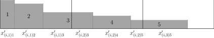
Figure 2: Illustration of bucket creation by Algorithm 1 for player $i$. Buckets are marked by solid lines. The value $x_{i3}$ is split into $x^{\prime}_{(i,1)3}$ and $x^{\prime}_{(i,2)3}$ and $x_{i5}$ is split into $x^{\prime}_{(i,2)5}$ and $x^{\prime}_{(i,3)5}$. For the other items we have $x^{\prime}_{(i,1)1}=x_{i1},x^{\prime}_{(i,1)2}=x_{i2},x^{\prime}_{(i,2)4}=x_{i4}$. Items are ordered in non-decreasing order by their prices.

Algorithm 1 first partitions $x$ into buckets creating a new assignment $x^{\prime}$, such that the sum of $x^{\prime}$ in each bucket is exactly 1 except possibly the last bucket of each player. Some items are split into two buckets. The process for one player is illustrated in Figure 2.

From the previous discussion, for every bucket $b$ we have $\sum_{j}x^{\prime}_{bj}\leq 1$. Also, $\sum_{b\in U}x^{\prime}_{bj}=1$ for every item $j$, which is implied by $\sum_{i\in\mathcal{A}}x_{ij}=1$ for all $j\in\mathcal{Q}$. Hence $x^{\prime}$ is inside the complete matching polytope for $V=\mathcal{Q}$. Using an algorithmic version of Carathéodory’s theorem (see e.g. Theorem 6.5.11 in [11]) we can in polynomial time decompose $x^{\prime}$ into a convex combination of polynomially many complete matchings for $V$.

In the algorithm we use an ordering $o_{i}$ for player $i$ such that $p_{io_{ij}}\geq p_{io_{i,j+1}}$, i.e. it is the descending order of items by their prices for player $i$. In particular this implies that the algorithm does not use the prices, only the order of items. Also note that Algorithm 1 could be made deterministic. Instead of picking a random matching we can pick the best one.

Let $\mathsf{Alg}_{i}(x)$ be the expected price that player $i$ pays. We know that $\mathsf{Alg}_{i}(x)\leq\mathsf{Val}_{i}(x)$, because the probability of assigning $j$ to $i$ is $x_{ij}$, but we don’t have equality in the expression, because some matchings might assign a price that is over the budget for some players. In the following lemma we bound $\mathsf{Alg}_{i}(x)$ from below.

Lemma 1.

Let $x$ be a solution to the assignment LP, $i\in\mathcal{A}$ and let $\alpha\geq 1$ be such that $\mathsf{Val}_{i}(x)=B_{i}/\alpha$. Let $a_{1}$ be the average price of items in the first bucket $b$ of player $i$, i.e. $a_{1}=\sum_{j}x^{\prime}_{bj}p_{bj}$. Let $r_{1}$ be the average price of items in $b$ that have price more than $\alpha a_{1}$. Then

$$\mathsf{Alg}_{i}(x)\geq\mathsf{Val}_{i}(x)\left(1-\frac{r_{1}}{4B_{i}}\right).$$

In particular, since $r_{i}\leq B_{i}$, Algorithm 1 gives a 3/4-approximation.

Proof.

The expected value of the solution $x^{*}$ for player $i$ is $\mathbb{E}[\mathsf{Val}_{i}(x^{*})]=\mathsf{Val}_{i}(x)$, because the probability of assigning item $j$ to player $i$ is $x_{ij}$. The problem with the assignment $x^{*}$ is that some players might go over the budget, so we cannot make use of the full value $\mathsf{Val}_{i}(x^{*})$. We now prove that we only lose $\frac{r_{1}}{4B_{i}}$-fraction of $\mathsf{Val}_{i}(x)$ by going over the budget of player $i$.

Note that $\alpha\geq 1$, since a solution to assignment LP never goes over the budget $B_{i}$. Let $a_{b}$ be the average price in bucket $b$. The matching picks at most one item from each bucket and suppose from each bucket $b$ it picks item of price more than $\alpha\cdot a_{b}$. Then since $\alpha\sum a_{b}=B_{i}$, the player would be assigned more than her budget. However, if we assume that all items within $b$-th bucket have price at most $\alpha\cdot a_{b}$, all maximum matchings assign price at most $B_{i}$ to player $i$. We thus define $p^{\prime}_{bj}$ to be $\min\{p_{bj},\alpha\cdot a_{b}\}$ and we get a new instance $\mathcal{J}$ with prices $p^{\prime}$ and buckets become the players of this instance. From the previous discussion we know no player goes over budget when using the fictional prices $p^{\prime}$, so $\mathsf{Val}_{i}^{\mathcal{J}}(x^{*})\leq B_{i}$. Thus $\mathsf{Alg}_{i}(x)$ can be lower-bounded by $\mathbb{E}[\mathsf{Val}_{i}^{\mathcal{J}}(x^{*})]=\mathsf{Val}_{i}^{\mathcal{J}}(x^{\prime})$. We now prove that $\mathsf{Val}_{i}^{\mathcal{J}}(x^{\prime})\geq(1-\frac{r_{1}}{4B_{i}})\mathsf{Val}_{i}(x)$.

Let $r_{b}$ be the average price of items in bucket $b$ with price above $\alpha\cdot a_{b}$ and let $q_{b}$ be the average price of the rest of the items in bucket $b$. Note that $q_{b}\geq r_{b+1}$. We let $x^{\prime}_{b}$ be the probability corresponding to $r_{b}$, i.e. the sum of all $x^{\prime}_{bj}$ where $p_{bj}>\alpha\cdot a_{b}$. Since $p_{ij}$ is changed to $\alpha\cdot a_{b}$ in $p^{\prime}$ for these items, the difference in price for bucket $b$ is $(r_{b}-\alpha a_{b})x^{\prime}_{b}$. The loss of value by going from $p$ to $p^{\prime}$ is thus

$$\mathsf{Val}_{i}(x)-\mathsf{Val}_{i}^{\mathcal{J}}(x^{\prime})=\sum_{b}(r_{b}-\alpha a_{b})x^{\prime}_{b}.$$

Since $a_{b}=(r_{b}-q_{b})x^{\prime}_{b}+q_{b}$, we have $(r_{b}-\alpha a_{b})x^{\prime}_{b}=(r_{b}-\alpha q_{b})x^{\prime}_{b}-(r_{b}-q_{b})\alpha{x^{\prime}_{b}}^{2}\leq(r_{b}-q_{b})(x^{\prime}_{b}-\alpha{x^{\prime}_{b}}^{2})$ where the last inequality follows from $\alpha\geq 1$. Since $q_{b}\geq r_{b+1}$, we get $(r_{b}-\alpha a_{b})x^{\prime}_{b}\leq(r_{b}-q_{b})(x^{\prime}_{b}-\alpha{x^{\prime}_{b}}^{2})\leq(r_{b}-r_{b+1})(x^{\prime}_{b}-\alpha{x^{\prime}_{b}}^{2})$. It follows that

$$\mathsf{Val}_{i}(x)-\mathsf{Val}_{i}^{\mathcal{J}}(x^{\prime})\leq\sum_{b}(r_{b}-r_{b+1})(x^{\prime}_{b}-\alpha{x^{\prime}_{b}}^{2}).$$

The maximum of $x^{\prime}_{b}-\alpha{x^{\prime}_{b}}^{2}$ is attained for $x^{\prime}_{b}=\frac{1}{2\alpha}$ and we get

$$\mathsf{Val}_{i}(x)-\mathsf{Val}_{i}^{\mathcal{J}}(x^{\prime})\leq\sum_{b}\frac{r_{b}-r_{b+1}}{4\alpha}\leq\frac{r_{1}}{4\alpha}$$

Hence

$$\mathsf{Alg}_{i}(x)\geq\mathsf{Val}_{i}^{\mathcal{J}}(x^{\prime})\geq\mathsf{Val}_{i}(x)-\frac{r_{1}}{4\alpha}=\mathsf{Val}_{i}(x)\left(1-\frac{r_{1}}{4B_{i}}\right)$$

which concludes the proof. ∎

4 Restricted Budget Allocation

In this section we consider the MBA problem with uniform budgets where the prices are restricted to be of the form $p_{ij}\in\{p_{j},0\}$. This is the so called restricted maximum budgeted allocation. Our main result is the following.

Theorem 3.

There is a $(3/4+c)$-approximation algorithm for restricted MBA for some constant $c>0$.

Since the budgets are uniform, we can assume that each player has a budget of $1$ by scaling. We refer to $p_{j}$ as the price of item $j$ and it is convenient to distinguish whether items have big or small prices. We let $\mathcal{B}=\{j:p_{j}\geq 1-\beta\}$ for some $\beta,1/3\geq\beta>0$ to be determined. $\mathcal{B}$ is the set of items of big price and let $\mathcal{S}$ denote the set of the remaining items (of small price).

A key concept for proving Theorem 3 is that of well-structured solutions; it allows us to use different techniques based on the structure of the solution to the configuration LP. In short, a solution $y$ is $(\epsilon,\delta)$-well-structured, if for at least $(1-\epsilon)$-fraction of players roughly half of their configurations contain a big item.

Definition 1.

A solution $y$ to the configuration LP is $(\epsilon,\delta)$-well-structured if

$$\Pr_{i}\left[\sum_{\mathcal{C}\subseteq\mathcal{Q}}|\mathcal{B}\cap\mathcal{C}|\cdot y_{i,\mathcal{C}}\not\in\left[\frac{1-\delta}{2},\frac{1+\delta}{2}\right]\right]\leq\epsilon,$$

where the probability is taken over a weighted distribution of players such that player $i$ is chosen with probability $\mathsf{Val}_{i}(y)/\mathsf{Val}(y)$.

We want to be able to switch from configuration LP to assignment LP without changing the well-structuredness of the solution. The following lemma shows that it is indeed possible.

Lemma 2.

Let $y$ be a well-structured solution to the configuration LP. Then there exists a solution $x$ to the assignment LP with $\mathsf{Val}_{i}(x)=\mathsf{Val}_{i}(y)$ such that

$$\sum_{\mathcal{C}\subseteq\mathcal{Q}}|\mathcal{B}\cap\mathcal{C}|\cdot y_{i,\mathcal{C}}\in\left[\frac{1-\delta}{2},\frac{1+\delta}{2}\right]\Leftrightarrow\sum_{j:j\in\mathcal{B}}x_{ij}\in\left[\frac{1-\delta}{2},\frac{1+\delta}{2}\right]$$

for all $i\in\mathcal{A}$. Furthermore, $x$ can be produced from $y$ in polynomial time.

Proof.

Note that we can assume that each configuration in $y$ contains at most 2 big items. If a configuration contains more than 2 big items, all but 2 big items can be removed without decreasing the objective value, since $2(1-\beta)\geq 1$ and thus the configuration remains over the budget.

We first modify $y$ to a new solution $y^{\prime}$ where each player does not have at the same time a configuration with 2 big items and a configuration with no big items. Solution $y^{\prime}$ is then projected to a solution $x$ to the assignment LP with desired properties.

Fix player $i$ and two configurations $\mathcal{C},\mathcal{C}^{\prime}$ such that $\mathcal{C}$ contains two big items and $\mathcal{C}^{\prime}$ contains no big items. We can assume that $y_{i\mathcal{C}}=y_{i\mathcal{C}^{\prime}}$, otherwise we can split the bigger fractional value into two and disregard one of them. We want to move the second big item from $\mathcal{C}$ into $\mathcal{C}^{\prime}$ without decreasing the objective value. This is done by moving back small items from $\mathcal{C}^{\prime}$.

Let us order the items in $\mathcal{C}^{\prime}$ by value in decreasing order $j_{1},\dots,j_{k}$. We move a big item from $\mathcal{C}$ to $\mathcal{C}^{\prime}$ and then move $j_{1},j_{2},\dots$ to $\mathcal{C}$ until it has profit at least 1 or we run out of items. Let $F$ and $F^{\prime}$ be the transformed configurations which arise from $\mathcal{C},\mathcal{C}^{\prime}$ respectively.

If the value of $\mathcal{C}^{\prime}$ is less than $\beta$, then we run out of items and the value of $F$ is at least $1-\beta+\sum_{j\in\mathcal{C}^{\prime}}p_{j}$ and the value of $F^{\prime}$ is at least $1-\beta>\beta$, so the objective value improved and $y$ is not an optimal solution, a contradiction. Hence we have that the value of $\mathcal{C}^{\prime}$ is at least $\beta$ and $F$ has value at least $1$.

It remains to prove that the value of $F^{\prime}$ is at least as big as the value of $\mathcal{C}^{\prime}$. In the above process we move a big item of value at least $1-\beta$ to $F^{\prime}$ and we now show that we move less in the other direction. Suppose towards contradiction that we moved more than $1-\beta\geq 2\beta$ to $F$, then we moved at least 2 small items and the last item added must have been of value at least $\beta$. But then only one such item is necessary, since $\mathcal{C}$ already contains a big item that has value of at least $1-\beta$.

Applying this procedure whenever we can, we end up with a modified solution $y^{\prime}$ to the configuration LP in which there is no player at the same time having a configuration containing two big items and a configuration with no big items. Also, $y^{\prime}$ is such that

$$\sum_{\mathcal{C}\subseteq\mathcal{Q}}|\mathcal{B}\cap\mathcal{C}|\cdot y_{i,\mathcal{C}}=\sum_{\mathcal{C}\subseteq\mathcal{Q}}|\mathcal{B}\cap\mathcal{C}|\cdot y^{\prime}_{i,\mathcal{C}},$$

because big items are only moved between configurations, so their contribution to the sums above is preserved.

The pairs of configurations $\mathcal{C},\mathcal{C}^{\prime}$ can be chosen in such a way that we only create polynomially many new configurations in total. To see this, let $T=\{\mathcal{C}_{1},\dots,\mathcal{C}_{k}\}$ be the configurations in $y$ that have two big items and let $S=\{\mathcal{C}^{\prime}_{1},\dots,\mathcal{C}^{\prime}_{\ell}\}$ be the configurations in $y$ with no big items. We process $T$ one by one. For each $\mathcal{C}_{j}\in T$ we try to move the second big item to the configurations $\mathcal{C}^{\prime}_{1},\dots,\mathcal{C}^{\prime}_{\ell}$ one by one. In the end we try at most $k\cdot\ell$ different pairs and each pair creates at most 2 new configurations. Since $k\cdot\ell$ is polynomial in the size of the instance, also the number of new configurations is polynomial.

Now we project $y^{\prime}$ to a solution $x$ to the assignment LP as follows: for every player $i$ and configuration $\mathcal{C}$, consider the items in $\mathcal{C}$ in non-increasing order according to $p_{ij}$. If the total value of $\mathcal{C}$ is at most $B_{i}$, the configuration $\mathcal{C}$ contributes $y^{\prime}_{i\mathcal{C}}$ to the value $x_{ij}$ for all items $j\in\mathcal{C}$. Otherwise the total value goes over the budget and only the first part of the ordered items that is below the budget gets contribution $y^{\prime}_{i\mathcal{C}}$ and the rest of the items gets contribution 0, except the one item that is only partially below the budget which gets some fraction between $0$ and $y^{\prime}_{i\mathcal{C}}$. In particular this means that big items get the full contribution $y^{\prime}_{i\mathcal{C}}$.

Let us now formalize the intuition given above. Let $j^{\prime}$ be the minimum index such that $\sum_{1\leq j\leq j^{\prime}}p_{ij}>B_{i}$. For all $j>j^{\prime}$, set $z_{ij\mathcal{C}}=0$, for all $j<j^{\prime}$ set $z_{ij\mathcal{C}}=y^{\prime}_{i\mathcal{C}}$ and set

$$z_{ij^{\prime}\mathcal{C}}=\frac{B_{i}-\sum_{1\leq j<j^{\prime}}p_{ij}}{p_{ij^{\prime}}}y^{\prime}_{i\mathcal{C}}.$$

Finally, we define

$$x_{ij}=\sum_{\mathcal{C}\subseteq\mathcal{Q}}z_{ij\mathcal{C}}.$$

We have $\mathsf{Val}(x)=\mathsf{Val}(y^{\prime})=\mathsf{Val}(y)$, since $\sum_{j}z_{ij\mathcal{C}}p_{ij}=w_{i}(\mathcal{C})y_{i\mathcal{C}}$, i.e. the contribution of each configuration is preserved by the projection.

The projection from $y^{\prime}$ to $x$ gives full contribution $y^{\prime}_{i\mathcal{C}}$ to the largest item in $\mathcal{C}$. If there are two big items in $\mathcal{C}$, the second big item does not get the full contribution. However, this happens only when $\sum_{\mathcal{C}\subseteq\mathcal{Q}}|\mathcal{B}\cap\mathcal{C}|\cdot y^{\prime}_{i,\mathcal{C}}>1$ and in this case all configurations in $y^{\prime}$ for player $i$ have a big item. Then $1\leq\sum_{j:j\in\mathcal{B}}x_{ij}$. However, if the total weight of big items in $y^{\prime}$ for player $i$ is less than 1, the same total weight is projected on $x$. We thus have

$$\sum_{j:j\in\mathcal{B}}x_{ij}=\sum_{\mathcal{C}\subseteq\mathcal{Q}}|\mathcal{B}\cap\mathcal{C}|\cdot y_{i,\mathcal{C}}$$

if $\sum_{\mathcal{C}\subseteq\mathcal{Q}}|\mathcal{B}\cap\mathcal{C}|\cdot y_{i,\mathcal{C}}\leq 1$ and otherwise $\sum_{j:j\in\mathcal{B}}x_{ij}>1$. This concludes the proof. ∎

In the next subsection in Lemma 5 we show that Algorithm 1 actually performs better then $3/4$ if the solution $x$ to the assignment LP is produced from a non-well-structured solution $y$ as in Lemma 2. In subsection 4.2 in Lemma 6 we show a new algorithm for well-structured solutions that also has an approximation guarantee strictly better than $3/4$. Finally, Lemma 5 and Lemma 6 immediately imply our main result of this section, i.e., Theorem 3.

4.1 Better analysis for non-well-structured solutions

We first show that Algorithm 1 performs well if not all players basically are fully assigned (fractionally).

Lemma 3.

Let $\varepsilon^{\prime}>0$ be a small constant and consider player $i$ such that $\mathsf{Val}_{i}(x)\leq 1-\varepsilon^{\prime}$. Then $\mathsf{Alg}_{i}(x)\geq\frac{3+\varepsilon^{\prime}/5}{4}\mathsf{Val}_{i}(x)$.

Proof.

For player $i$, select the largest $Q_{i}$ such that

$$Q_{i}=\sum_{j}x_{ij}q_{ij},\qquad\mbox{ where }q_{ij}=\min\{p_{ij},Q_{i}\}.$$

Note that such a $Q_{i}$ always exists, since $0$ always satisfies the equation. Let $f_{i}(z)=\sum_{j}x_{ij}\min\{p_{ij},z\}$ and note that $f_{i}(z)$ is a continuous function. We have $f_{i}(1)=\mathsf{Val}_{i}(x)<1$ and $f_{i}(0)=0$ and we want to find the largest $Q_{i}$, such that $f_{i}(Q_{i})=Q_{i}$.

If we substitute prices $p_{ij}$ with $q_{ij}=\min\{p_{ij},Q_{i}\}$, the ordering of the items for a player by the price stays the same. Thus Algorithm 1 produces the same result no matter which one of the two prices we use. Let $D_{i}$ denote the difference $\sum_{j}x_{ij}(p_{ij}-q_{ij})=\mathsf{Val}_{i}(x)-Q_{i}$. We do case distinction based on the size of $D_{i}$.

Case $D_{i}>\frac{\varepsilon^{\prime}}{5}\mathsf{Val}_{i}(x)$:

By Lemma 1, if we run Algorithm 1 on $x$ but use values $q_{ij}$ and budget $Q_{i}$ in the analysis, we get $\mathsf{Alg}_{i}(x)\geq\frac{3}{4}Q_{i}$. In order to improve this we use the fact that $q_{ij}<p_{ij}$ only for at most one unit of the largest items. If already more than one unit of items is at least $Q_{i}$, then we have $f_{i}(Q_{i})>Q_{i}$. Since $f_{i}(1)<1$ and $f_{i}$ is continuous, $Q_{i}$ is not the largest solution to $f_{i}(z)=z$, a contradiction.

Moreover, since the assignment according to the analysis with respect to $q$ does not violate the budget $Q_{i}$, we can always add back the difference $p_{ij}-q_{ij}$ if $j$ is assigned to $i$ without violating the budget $B_{i}$, since $p_{ij}-q_{ij}\leq B_{i}-Q_{i}$. We are not losing a quarter from the difference $D_{i}$, so we have an advantage of $D_{i}/4>\frac{\varepsilon^{\prime}}{20}\mathsf{Val}_{i}(x)$. Formally, the expected profit is

$$\frac{3}{4}Q_{i}+D_{i}=\frac{3}{4}(Q_{i}+D_{i})+D_{i}/4=\frac{3}{4}\mathsf{Val}_{i}(x)+D_{i}/4,$$

which is at least $\left(\frac{3}{4}+\frac{\varepsilon^{\prime}}{20}\right)\mathsf{Val}_{i}(x)$.

Case $D_{i}\leq\frac{\varepsilon^{\prime}}{5}\mathsf{Val}_{i}(x)$:

In this case we apply Lemma 1 with prices $q$ and budget $1$. Now since $Q_{i}$ is bounded away from $1$, $\mathsf{Alg}_{i}(x)$ is more than $3/4Q_{i}$. Formally,

$$\mathsf{Alg}_{i}(x)\geq(1-Q_{i}/4)Q_{i}=(1-Q_{i}/4)\mathsf{Val}_{i}(x)-(1-Q_{i}/4)D_{i}\geq(1-Q_{i}/4)\mathsf{Val}_{i}(x)-D_{i}.$$

As $Q_{i}\leq\mathsf{Val}_{i}(x)\leq 1-\varepsilon^{\prime}$,

$$\mathsf{Alg}_{i}(x)\geq\left(1-\frac{1-\varepsilon^{\prime}}{4}\right)\mathsf{Val}_{i}(x)-D_{i}\geq\left(1-\frac{1-\varepsilon^{\prime}/5}{4}\right)\mathsf{Val}_{i}(x)=\frac{3+\varepsilon^{\prime}/5}{4}\mathsf{Val}_{i}(x).$$

∎

From the above claim, we can see that the difficult players to round are those that have an almost full budget. Furthermore, we show in the following lemma that such players must have a very special fractional assignment in order to be difficult to round.

Lemma 4.

Let $\delta>0$ be a small constant, $\beta$ be such that $\delta/4\leq\beta$ and consider a player $i$ such that $\mathsf{Val}_{i}(x)\geq 1-\delta^{2}/8$ and $\sum_{j:j\in\mathcal{B}}x_{ij}\not\in\left[\frac{1-\delta}{2},\frac{1+\delta}{2}\right]$. Then $\mathsf{Alg}_{i}(x)\geq\frac{3+\delta^{2}/64}{4}\mathsf{Val}_{i}(x)$.

Proof.

If the average in the first bucket is more than $\frac{3+\delta^{2}/64}{4}\mathsf{Val}_{i}(x)$ then we are done, since assigning a random item from that bucket gives sufficient profit. If $r_{1}\leq 1-\delta^{2}/16$, Lemma 1 already implies the claim. Therefore assume from now on that $r_{1}\geq 1-\delta^{2}/16$ and $r_{2}\leq\frac{3+\delta^{2}/16}{4}$, so $r_{1}-r_{2}\geq 1/8$, since $\delta$ is small.

Select $\alpha\geq 1$ such that $\mathsf{Val}_{i}(x)=1/\alpha$. In the proof of Lemma 1 we have that the expected decrease in value compared to $\mathsf{Val}_{i}(x)$ in our rounding is at most

$$\sum_{b}(r_{b}-r_{b+1})(x^{\prime}_{b}-\alpha{x^{\prime}_{b}}^{2}).$$

This can be rewritten as

$$(r_{1}-r_{2})(x^{\prime}_{1}-\alpha{x^{\prime}_{1}}^{2})+\sum_{b\geq 2}(r_{b}-r_{b+1})(x^{\prime}_{b}-\alpha{x^{\prime}_{b}}^{2}) \leq(r_{1}-r_{2})(x^{\prime}_{1}-\alpha{x^{\prime}_{1}}^{2})+(r_{2}-r_{n})\cdot\frac{1}{4\alpha}$$

$$\leq 1/8(x^{\prime}_{1}-\alpha{x^{\prime}_{1}}^{2})+7/8\cdot\frac{1}{4\alpha}.$$

The last inequality follows from $(x^{\prime}_{1}-\alpha{x^{\prime}_{1}}^{2})\leq\frac{1}{4\alpha}$ and $r_{1}-r_{2}\geq 1/8$.

We now prove that $x^{\prime}_{1}$ can not be close to $1/2$. The probability $x^{\prime}_{1}$ corresponds to items in the first bucket that have value at least $\alpha a_{1}$. Suppose towards contradiction that more than $\delta^{2}/(16\beta)$-fraction of these items are not big items, so they have value at most $1-\beta$. Then $r_{1}<1-\frac{\delta^{2}}{16\beta}\cdot\beta=1-\delta^{2}/16$, a contradiction. This means that $x^{\prime}_{1}=(\sum_{j\in\mathcal{B}}x_{ij})+\gamma$, where $\gamma\in[0,\delta^{2}/(16\beta)]$. By $\beta\geq\delta/4$, $\gamma\in[0,\delta/4]$. Since $\sum_{j\in\mathcal{B}}x_{ij}\not\in\left[\frac{1-\delta}{2},\frac{1+\delta}{2}\right]$, we have $x^{\prime}_{1}\not\in\left[\frac{1-\delta/2}{2},\frac{1+\delta/2}{2}\right]$.

We now use the fact that $x^{\prime}_{i}$ is bounded away from $1/2$ to prove that the loss in the rounding is less than $1/4$. For function $z-z^{2}$ the maximum is attained for $z=1/2$, so $z$ bounded away from $1/2$ by gives values bounded away from maximum which is 1/4. For function $z-\alpha z^{2}$ the maximum is attained very close to $1/2$ provided that $\alpha$ is close to $1$. Again, $z$ bounded away from $1/2$ gives values bounded away from the maximum. In the rest of the proof we formalize this intuition.

The maximum for the function $z(1-\alpha z)$ is attained for $z=\frac{1}{2\alpha}$ and we can prove that $\frac{1}{2\alpha}\in\left[\frac{1-\delta/2}{2},\frac{1+\delta/2}{2}\right]$. Since $\alpha\geq 1$, it only remains to prove that $\frac{1}{2\alpha}\geq\frac{1-\delta/2}{2}$. By $1/\alpha\geq 1-\delta^{2}/8$,

$$\frac{1}{2\alpha}\geq\frac{1-\delta^{2}/8}{2}>\frac{1-\delta/2}{2}.$$

The function $z-\alpha z^{2}$ is symmetric around $\frac{1}{2\alpha}$ and this value is closer to the beginning of the interval $\left[\frac{1-\delta/2}{2},\frac{1+\delta/2}{2}\right]$, so the maximum of $x^{\prime}_{1}-\alpha{x^{\prime}_{1}}^{2}$ is attained when $x^{\prime}_{1}=\frac{1-\delta/2}{2}$.

We have that

$$x^{\prime}_{1}-\alpha{x^{\prime}_{1}}^{2}\leq x^{\prime}_{1}-{x^{\prime}_{1}}^{2}=\frac{1-\delta^{2}/4}{4}\leq\frac{1}{4}{(1-\delta^{2}/8)}^{2}.$$

Since $1-\delta^{2}/8\leq\frac{1}{\alpha}$,

$$x^{\prime}_{1}-\alpha{x^{\prime}_{1}}^{2}\leq\frac{1-\delta^{2}/8}{4\alpha}.$$

We can finally bound the decrease in our rounding to be at most

$$r_{1}\left(\frac{1}{8}\cdot\frac{1-\delta^{2}/8}{4\alpha}+\frac{7}{8}\cdot\frac{1}{4\alpha}\right)=\frac{r_{1}(1-\delta^{2}/64)}{4\alpha}.$$

The claim follows from the fact that $r_{1}\leq 1$. ∎

From Lemma 3 and Lemma 4 we have that as soon as a weighted $\epsilon$-fraction (weight of player $i$ is $\mathsf{Val}_{i}(y)$) of the players satisfies the conditions of either lemma, we get a better approximation guarantee than 3/4. Therefore, when a solution $y$ to the configuration LP is not $(\epsilon,\delta)$-well-structured, we use Lemma 2 to produce a solution $x$ to the assignment LP for which $\epsilon$-fraction of players satisfies either conditions of Lemma 3 or Lemma 4. Hence we have the following lemma:

Lemma 5.

Given a solution $y$ to the configuration LP which is not $(\epsilon,\delta)$-well-structured and $\beta\geq\delta/4$, we can in polynomial time find a solution with expected value at least $\frac{3+\epsilon\delta^{2}/64}{4}\mathsf{Val}(y)$.

Proof.

Let $x$ be a solution to the assignment LP produced from $y$ as in Lemma 2. Then more than weighted $\epsilon$-fraction of players have $\sum_{j:j\in\mathcal{B}}x_{ij}\not\in\left[\frac{1-\delta}{2},\frac{1+\delta}{2}\right]$.

According to Lemma 3 using $\epsilon^{\prime}=\delta^{2}/8$, we have $\mathsf{Alg}_{i}(x)\geq\frac{3+\delta^{2}/40}{4}\mathsf{Val}_{i}(x)$ if $\mathsf{Val}_{i}(x)\leq 1-\delta^{2}/8$. By Lemma 4, using $\beta\geq\delta/4$ implies $\mathsf{Alg}_{i}(x)\geq\frac{3+\delta^{2}/64}{4}\mathsf{Val}_{i}(x)$ if $\mathsf{Val}_{i}(x)\geq 1-\delta^{2}/8$ and $\sum_{j:j\in\mathcal{B}}x_{ij}\not\in\left[\frac{1-\delta}{2},\frac{1+\delta}{2}\right]$. Hence for weighted $\epsilon$-fraction of players we get $\mathsf{Alg}_{i}(x)\geq\frac{3+\delta^{2}/64}{4}\mathsf{Val}_{i}(x)$, so the total gain is at least $\frac{3+\epsilon\delta^{2}/64}{4}\mathsf{Val}(y)$. ∎

4.2 Algorithm for well-structured solutions

Here, we devise a novel algorithm that gives an improved approximation guarantee for $(\epsilon,\delta)$-well-structured instances when $\epsilon$ and $\delta$ are small constants.

Lemma 6.

Let $1-\beta$ be the threshold for the big items. Given a solution $y$ to the configuration LP that is $(\epsilon,\delta)$-well-structured, we can in (randomized) polynomial time find a solution with expected value at least $(1-\delta)^{2}(1-\beta-\epsilon)\cdot\frac{25}{32}\mathsf{Val}(y)$.

To prove the above lemma we first give the algorithm and then its analysis.

Algorithm.

The algorithm constructs a slightly modified version $y^{\prime}$ of the optimal solution $y$ to the configuration LP. Solution $y^{\prime}$ is obtained from $y$ in three steps. First, remove all players $i$ with $\sum_{\mathcal{C}\subseteq\mathcal{Q}}|\mathcal{B}\cap\mathcal{C}|y_{i,\mathcal{C}}\not\in\left[\frac{(1-\delta)}{2},\frac{(1+\delta)}{2}\right]$. As solution $y$ is $(\epsilon,\delta)$-well-structured, this step decreases the value of the solution by at most $\epsilon\mathsf{Val}(y)$.

Second, change $y$ as in the proof of Lemma 2 by getting rid of configurations with 2 big items without losing any objective value. Then remove all small items from the configurations containing big items. After this step, we have the property that big items are alone in a configuration. We call such configurations big and the remaining ones small. Moreover, we have decreased the value by at most $\beta\mathsf{Val}(y)$ because each big item has value at least $1-\beta$ and each configuration has value at most $1$. In the third step, we scale down the fractional assignment of configurations (if necessary), so as to ensure that $\sum_{\mathcal{C}:\mathcal{C}\cap\mathcal{B}=\emptyset}y^{\prime}_{i,\mathcal{C}}\leq 1/2$ for each player $i\in\mathcal{A}$. As remaining players are assigned big configurations with a total fraction at least $(1-\delta)/2$ and therefore small configurations with a total fraction at most $(1+\delta)/2$, this may decrease the value by a factor $1/(1+\delta)>1-\delta$.

In summary, we have obtained a solution $y^{\prime}$ for the configuration LP so that each configuration either contains a single big item or small items; for each remaining player the configurations with big items constitute a fraction in $\left[\frac{(1-\delta)}{2},\frac{(1+\delta)}{2}\right]$ and small configurations constitute a fraction of at most $1/2$. Moreover, $\mathsf{Val}(y^{\prime})\geq(1-\beta-\epsilon)(1-\delta)\mathsf{Val}(y)$.

The algorithm now works by rounding $y^{\prime}$ in two phases; in the first phase we assign big items and in the second phase we assign small items.

The first phase works as follows. Let $x^{\prime}$ be the solution to the assignment LP from Lemma 2 applied on $y^{\prime}$ and note that $\mathsf{Val}(x^{\prime})=\mathsf{Val}(y^{\prime})$. Consider the bipartite graph where we have a vertex $a_{i}$ for each player $i\in\mathcal{A}$; a vertex $b_{j}$ for each big item $j\in\mathcal{B}$; and an edge of weight $x^{\prime}_{ij}$ between vertices $a_{i}$ and $b_{j}$. Note that a matching in this graph naturally corresponds to an assignment of big items to players. We shall find our matching/assignment of big items by using Theorem 2. Note that by the property of that theorem we have that (i) each big item $j$ is assigned with probability $\sum_{i}x^{\prime}_{ij}$ and (ii) the probability that two players $i$ and $i^{\prime}$ are assigned big items is negatively correlated, i.e., it is at most $\left(\sum_{j\in\mathcal{B}}x^{\prime}_{ij}\right)\cdot\left(\sum_{j\in\mathcal{B}}x^{\prime}_{i^{\prime}j}\right)$. These two properties are crucial in the analysis of our algorithm. It is therefore important that we assign the big items according to a distribution that satisfies the properties of Theorem 2.

After assigning big items, our algorithm proceeds in the second phase to assign the small items as follows. First, obtain an optimal solution $x^{(2)}$ to the assignment LP for the small items together with the players that were not assigned a big item in the first phase; these are the items that remain and the players for which the budget is not saturated with value at least $1-\beta$. Then we obtain an integral assignment (of the small items) of value at least $\frac{3}{4}\mathsf{Val}(x^{(2)})$ by using Algorithm 1.

Analysis.

Let $\mathcal{A}_{j}$ be all the players $i$ for which $x^{\prime}_{ij}>0$. Let $x^{*}$ denote the integral assignment found by the algorithm. Note that the expected value of $x^{*}$ (over the randomly chosen assignment of big items) is:

$$\mathbb{E}[\mathsf{Val}(x^{*})] =\mathbb{E}\left[\sum_{j\in\mathcal{B}}\sum_{i\in\mathcal{A}_{j}}x^{\prime}_{ij}p_{j}+\frac{3}{4}\mathsf{Val}(x^{(2)})\right]=\sum_{j\in\mathcal{B}}\sum_{i\in\mathcal{A}_{j}}x^{\prime}_{ij}p_{j}+\frac{3}{4}\mathbb{E}[\mathsf{Val}(x^{(2)})].$$

We now analyze the second term, i.e., the expected optimal value of the assignment LP where we are only considering the small items and the set of players $T\subseteq\mathcal{A}$ that were not assigned big items in the first phase. Then a solution $z$ to the assignment LP can be obtained by scaling up the fractional assignments of the small items assigned to players in $T$ according to $x^{\prime}$ by up to a factor of $2$ while maintaining that an item is assigned at most once. In other words, $z_{ij}=\min\left[1,\sum_{i\in\mathcal{A}_{j}\cap T}2x^{\prime}_{ij}\right]$ and $z$ is a feasible solution to the assignment LP, because we have $\sum_{j\in\mathcal{S}}x^{\prime}_{ij}p_{j}\leq 1/2$.

Thus we have that the expected value of the optimal solution to the assignment LP is by linearity of expectation is at least $\mathbb{E}_{T}[\mathsf{Val}(x^{(2)})]\geq\sum_{j\in\mathcal{S}}p_{j}\cdot\mathbb{E}_{T}\left[\min\left[1,\sum_{i\in\mathcal{A}_{j}\cap T}2x^{\prime}_{ij}\right]\right]$.

We continue by analyzing the expected fraction of a small item present in the constructed solution to the assignment LP. In this lemma we use that the randomly selected matching of big items has negative correlation. To see why this is necessary, consider a small item $j\in\mathcal{S}$ and suppose that $j$ is assigned to two players $A$ and $B$ both with a fraction $1/2$, i.e., $x^{\prime}_{Aj}=x^{\prime}_{Bj}=1/2$. As the instance is well-structured both $A$ and $B$ are roughly assigned half a fraction of big items; for simplicity assume it to be exactly $1/2$. Note that in this case we have that $\min\left[1,\sum_{i\in\mathcal{A}_{j}\cap T}2x^{\prime}_{ij}\right]$ is equal to $1$ if not both $A$ and $B$ are assigned a big item and $0$ otherwise. Therefore, on the one hand, if the event that $A$ is assigned a big item and the event that $B$ is assigned a big item were perfectly correlated then we would have $\mathbb{E}_{T}\left[\min\left[1,\sum_{i\in\mathcal{A}_{j}\cap T}2x^{\prime}_{ij}\right]\right]=1/2$. On the other hand, if those events are negatively correlated then $\mathbb{E}_{T}\left[\min\left[1,\sum_{i\in\mathcal{A}_{j}\cap T}2x^{\prime}_{ij}\right]\right]\geq 3/4$, as in this case the probability that both $A$ and $B$ are assigned big items is at most $1/4$.

Lemma 7.

For every $j\in\mathcal{S}$, $\mathbb{E}_{T}\left[\min\left[1,\sum_{i\in\mathcal{A}_{j}\cap T}2x^{\prime}_{ij}\right]\right]\geq(1-\delta)\frac{3}{4}\sum_{i\in\mathcal{A}_{j}}x^{\prime}_{ij}$.

Proof.

We slightly abuse notation and also denote by $T$ the event that the players in $T\subseteq\mathcal{A}$ were those that were not assigned big items. Let also $x(T)=\min\left[1,\sum_{k\in\mathcal{A}_{j}\cap T}2x^{\prime}_{kj}\right]$ for the considered small item $j$. With this notation,

$$\mathbb{E}_{T}\left[\min\left[1,\sum_{i\in\mathcal{A}_{j}\cap T}2x^{\prime}_{ij}\right]\right]=\sum_{T\subseteq\mathcal{A}}\Pr[T]\cdot x(T).$$

We shall show that we can lower bound this quantity by assuming that $j$ is only fractionally assigned to two players. Indeed, suppose that $j$ is fractionally assigned to more than two players. Then there must exist two players, say $i$ and $i^{\prime}$, so that $0<x^{\prime}_{ij}<1/2$ and $0<x^{\prime}_{i^{\prime}j}<1/2$; the fractional assignment of a small item to some player never exceeds $1/2$ by construction of $y^{\prime}$ and $x^{\prime}$. We can write $\sum_{T\subseteq\mathcal{A}}\Pr[T]\cdot x(T)$ as

$$\sum_{T\subseteq\mathcal{A}\setminus\{i,i^{\prime}\}}( \Pr[T]\cdot x(T)+\Pr[T\cup\{i\}]\cdot x(T\cup\{i\})+\Pr[T\cup\{i^{\prime}\}]\cdot x(T\cup\{i^{\prime}\})$$ (1)

$$+\Pr[T\cup\{i,i^{\prime}\}]\cdot x(T\cup\{i,i^{\prime}\}))$$

Note that if we shift some amount of fractional assignment from $x^{\prime}_{ij}$ to $x^{\prime}_{i^{\prime}j}$ (or vice-versa) then $x(T)$ and $x(T\cup\{i,i^{\prime}\})$ do not change. We shall now analyze the effect such a shift has on the sums $\sum_{T\subseteq\mathcal{A}\setminus\{i,i^{\prime}\}}\Pr[T\cup\{i\}]\cdot x(T\cup\{i\})$ and $\sum_{T\subseteq\mathcal{A}\setminus\{i,i^{\prime}\}}\Pr[T\cup\{i^{\prime}\}]\cdot x(T\cup\{i^{\prime}\})$. Note that after this shift $x^{\prime}$ might not be a valid solution to the assignment LP, namely we might go over the budget for some players. However, our goal is only to prove a lower-bound on $\mathbb{E}[\mathsf{Val}(x^{(2)}]$.

For this purpose let $F_{i}$ denote the probability that the set $T$ is selected such that the value of $x(T\cup\{i\})$ is strictly less than $1$, i.e.,

$$F_{i}:=\sum_{T\subseteq\mathcal{A}\setminus\{i,i^{\prime}\}:x(T\cup\{i\})<1}\Pr[T\cup\{i\}].$$

Similarly we define $G_{i}$ for sets where $x(T\cup\{i\})$ is exactly 1, i.e.,

$$G_{i}:=\sum_{T\subseteq\mathcal{A}\setminus\{i,i^{\prime}\}:x(T\cup\{i\})=1}\Pr[T\cup\{i\}].$$

The definition of $F_{i^{\prime}}$ and $G_{i^{\prime}}$ is analogous. Note that if we, on the one hand, decrease $x^{\prime}_{ij}$ by a small $\eta$ and increase $x^{\prime}_{i^{\prime}j}$ by $\eta$, this changes (1) by $\eta(-F_{i}-G_{i}+F_{i^{\prime}})$. On the other hand, if we increase $x^{\prime}_{ij}$ and decrease $x^{\prime}_{i^{\prime}j}$ by $\eta$, then (1) changes by $\eta(F_{i}-F_{i^{\prime}}-G_{i^{\prime}})$. We know that one of $\eta(F_{i}-F_{i^{\prime}})$ and $\eta(-F_{i}+F_{i^{\prime}})$ is non-positive, so either $\eta(-F_{i}-G_{i}+F_{i^{\prime}})$ or $\eta(F_{i}-F_{i^{\prime}}-G_{i^{\prime}})$ are non-positive as well.

After the small change by $\eta$, $F_{i}$ increases by $G_{i}$ or $F_{i^{\prime}}$ by $G_{i^{\prime}}$, so further changes in the same direction will be also non-positive. We can therefore either shift fraction of $x^{\prime}_{ij}$ to $x^{\prime}_{i^{\prime}j}$ (or vice versa) without increasing (1) until one of the variables either becomes $0$ or $1/2$. If it becomes $0$ then we repeat with one less fractionally assigned small item and if it becomes $1/2$ then we repeat by considering two other players where $j$ is fractionally assigned strictly between $0$ and $1/2$.

By repeating the above process, we may thus assume that $j$ is fractionally assigned to at most two players say $1$ and $2$ and $x^{\prime}_{1j},x^{\prime}_{2j}\leq 1/2$. We therefore have that (1) is equal to

$$\Pr[1,2\not\in T]\cdot 0+\Pr[1\in T,2\not\in T]\cdot 2x^{\prime}_{1j}+\Pr[1\not\in T,2\in T]\cdot 2x^{\prime}_{2j}+\Pr[1,2\in T]\cdot\min[1,2x^{\prime}_{1j}+2x^{\prime}_{2j}]$$

It is clear that the above expression is minimized whenever $\Pr[1,2\in T]$ is maximized; however, since our distribution over the assignments of big items is negatively correlated and it preserves the marginals (which are at most $(1+\delta)/2$), it holds that $\Pr[1,2\in T]\leq\frac{(1-\delta)^{2}}{4}$(since the worst case is that $\Pr[1\in T]=\Pr[2\in T]=\frac{1-\delta}{2}$), and hence one can see that the above expression is at least

$$\left(\frac{1-\delta}{2}-\frac{(1-\delta)^{2}}{4}\right)2x^{\prime}_{1j}+\left(\frac{1-\delta}{2}-\frac{\left(1-\delta\right)^{2}}{4}\right)2x^{\prime}_{2j}+\frac{(1-\delta)^{2}}{4}\min[1,2x^{\prime}_{1j}+2x^{\prime}_{2j}]=$$

$$\frac{1+\delta}{2}\frac{1-\delta}{2}\cdot 2x^{\prime}_{1j}+\frac{1+\delta}{2}\frac{1-\delta}{2}\cdot 2x^{\prime}_{2j}+\frac{(1-\delta)^{2}}{4}\min[1,2x^{\prime}_{1j}+2x^{\prime}_{2j}]$$

which is at least

$$\frac{2-2\delta^{2}}{4}(x^{\prime}_{1j}+x^{\prime}_{2j})+\frac{1-2\delta+\delta^{2}}{4}(x^{\prime}_{1j}+x^{\prime}_{2j})\geq(1-\delta)\frac{3}{4}(x^{\prime}_{1j}+x^{\prime}_{2j}).$$

∎

Let us now see how it implies Lemma 6. We have that $\mathbb{E}[\mathsf{Val}(x^{*})]$ is equal to

$$\sum_{j\in\mathcal{B}}\sum_{i\in\mathcal{A}_{j}}x^{\prime}_{ij}p_{j}+\frac{3}{4}\mathbb{E}[\mathsf{Val}(x^{(2)})]\geq\ \sum_{j\in\mathcal{B}}\sum_{i\in\mathcal{A}_{j}}x^{\prime}_{ij}p_{j}+(1-\delta)\left(\frac{3}{4}\right)^{2}\sum_{j\in\mathcal{S}}\sum_{i\in\mathcal{A}_{j}}x^{\prime}_{ij}p_{j}.$$

As $\sum_{j\in\mathcal{B}}x^{\prime}_{ij}\geq\frac{1-\delta}{2}$ for every remaining player, we have

$$\frac{\mathbb{E}[\mathsf{Val}(x^{*})]}{\mathsf{Val}(x^{\prime})}\geq(1-\delta)\left(\frac{1}{2}+\frac{1}{2}\frac{9}{16}\right)=(1-\delta)\frac{25}{32}.$$

Lemma 6 now follows from that $\mathsf{Val}(x^{\prime})\geq(1-\beta-\epsilon)(1-\delta)\mathsf{Val}(y)$. We have proved Lemmas 5 and 6, which in turn imply Theorem 3 and our analysis is concluded.

5 Assigning Big Items

In this section, we show how to find a matching in a bipartite graph $G=(A,B,E)$ such that, for any set of vertices $S\subset A$, the probability that all the vertices of the set are matched is negatively correlated. We use the dependent rounding scheme of Gandhi et al. [9]. Because our precise goal differs from what they consider, we must slightly modify their analysis.

Definition 2.

Let $G=((A,B),E)$ be a bipartite graph with edge weights $x:E\rightarrow[0,1]$. We say that $G$ is a normal bipartite graph if for all $i\in A\cup B,~{}\sum_{j:(i,j)\in E}x_{ij}\leq 1$.

Note that $|A|$ and $|B|$ may not be equal. Suppose we have a randomized algorithm that produces a matching $M$. Let $X_{ij}$ denote the random variable that is 1 if edge $(i,j)$ belongs to $M$ and is 0 otherwise. Let $X_{i}$ denote the random variable that is 1 if vertex $i$ is matched in $M$ and 0 otherwise. We will show that there is a randomized algorithm to generate a matching $M$ such that the following properties hold.

• (P1): Marginal Distribution. For every vertex $i\in A\cup B$, $\Pr[X_{i}=1]=\sum_{j:(i,j)\in E}x_{ij}$.

• (P2): Negative Correlation. Let $S\subseteq A$.

  $$\Pr[\bigwedge_{i\in S}(X_{i}=1)] \leq \prod_{i\in S}\Pr[X_{i}=1].$$

Theorem 2.

If $G=((A,B),E)$ is a normal bipartite graph, then there is an efficient, randomized algorithm that generates a matching $M$ satisfying properties (P1) and (P2).

5.1 Algorithm and Proof of Theorem 2

We show that the dependent rounding scheme from [9] yields a matching algorithm that has the desired properties. We include the algorithm here for completeness. First, we give a short description.

The initial step of the algorithm is to remove all cycles from $G$ while preserving the sums at each vertex. In other words, it first preprocesses the $y_{ij}$ values (note that initially, $y_{ij}=x_{ij}$ for all edges in $G$) so that for each vertex $i\in A\cup B$, the value $\sum_{j:(i,j)\in E}y_{ij}$ is preserved, but the resulting graph contains no cycles. This can be done since $G$ is bipartite and may contain only even cycles, and is implemented in Step 3 of the algorithm.

After Step 3, the graph $G$ has been modified so that it no longer contains cycles. However, it may be the case that some of the $y_{ij}$ values are fractional. Our goal is to make all of these values integral, so that the $y_{ij}$ values correspond to a matching and the sums of the values corresponding to the edges adjacent a vertex are preserved in expectation. It is important to note that these sums may be less than 1. To obtain a matching from an acyclic graph, we use the method from [9]. We choose a path (which can be either even or odd in length) and divide this path into two matchings. The current $y_{ij}$ edge values restrict how much the edges can be increased or decreased (we never want any $y_{ij}$ value to exceed 1 or to be negative). We use these bounds to increase and decrease the $y_{ij}$ values in this path so as to preserve the expected value of the sums of the $y_{ij}$ values adjacent to a vertex.

Matching Algorithm Input: A normal bipartite graph $G=((A,B),E)$ with edge weights $x:E\rightarrow(0,1)$. Output: A matching $M\subset E$. 1. Initialize each edge weight with value $y_{ij}:=x_{ij}$. 2. If $y_{ij}=1$, then add edge $ij$ to the matching $M$. If $y_{ij}=0$, then delete edge $(i,j)$ from $G$. 3. Remove all cycles: A cycle $C$ can be decomposed into two matchings, $M_{1}$ and $M_{2}$. Let $\alpha=\min_{h\ell\in C}x_{h\ell}$ and without loss of generality, assume that $(i,j)\in M_{1}$, where $\alpha=x_{ij}$. • Set $y_{ij}:=y_{ij}-\alpha$ for all $(i,j)\in M_{1}$ and $y_{ij}:=y_{ij}+\alpha$ for all $(i,j)\in M_{2}$. • If $y_{ij}=1$, add edge $(i,j)$ to $M$. Delete all edges with integral $y_{ij}$ values from $G$.
(Note that this procedure does not change the fractional degree at any vertex.) 4. While $G$ is non-empty: Find a maximal path $P$ in $G$. • Divide $P$ into matchings $M_{1}$ and $M_{2}$. • Choose $\alpha$ and $\beta$ as follows: $\alpha=\min\{\gamma>0:(\exists(i,j)\in M_{1}:y_{ij}+\gamma=1)\bigvee(\exists(i,j)\in M_{2}:y_{ij}-\gamma=0)\}$; $\beta=\min\{\beta>0:(\exists(i,j)\in M_{1}:y_{ij}-\gamma=1)\bigvee(\exists(i,j)\in M_{2}:y_{ij}+\gamma=0)\}$. • With probability $\beta/(\alpha+\beta)$, set: $y_{ij}:=y_{ij}+\alpha$ for all $(i,j)\in M_{1}$ and $y_{ij}:=y_{ij}-\alpha$ for all $(i,j)\in M_{2}$. • With probability $\alpha/(\alpha+\beta)$, set: $y_{ij}:=y_{ij}-\beta$ for all $(i,j)\in M_{1}$ and $y_{ij}:=y_{ij}+\beta$ for all $(i,j)\in M_{2}$. • If $y_{ij}=1$, add edge $(i,j)$ to $M$. Delete all edges with integral $y_{ij}$ values from $G$.

5.2 Analysis

We note that the Matching Algorithm takes no more than $|E|$ rounds. This is because at each step, at least one edge becomes integral and is therefore removed from the edge set.

Lemma 8.

Property (P1) holds.

Proof.

Suppose the algorithm runs $t$ iterations of Step 4. Fix edge $(i,j)\in E$. Let $Y_{ij,k}$ denote the value of $y_{ij}$ right before iteration $k$. We will show that:

$$\forall k\geq 1,~{}\mathbbm{E}[Y_{ij,k+1}]=\mathbbm{E}[Y_{ij,k}].$$ (2)

Note that $Y_{ij,1}$ denotes the value of $y_{ij}$ after the last execution of Step 3 and before the first execution of Step 4. Then we have $\Pr[X_{ij}=1]=\mathbbm{E}[Y_{ij,t}]=\mathbbm{E}[Y_{ij,1}]$. Note that $\sum_{j:(i,j)\in E}x_{ij}=\sum_{j:(i,j)\in E}Y_{ij,1}$, since in removing cycles, the degree sums do not change.

Suppose edge $(i,j)\notin P$ where $P$ is the path chosen in round $k$. Then Equation (2) holds. If edge $(i,j)\in P$ and in $M_{1}$, then we have:

$$\mathbbm{E}[Y_{ij,k+1}] = \frac{\beta}{\alpha+\beta}(\mathbbm{E}[Y_{ij,k}]+\alpha)+\frac{\alpha}{\alpha+\beta}(\mathbbm{E}[Y_{ij,k}]-\beta)$$ (3)

$$= \mathbbm{E}[Y_{ij,k}].$$ (4)

If edge $(i,j)\in P$ and in $M_{2}$, then we have:

$$\mathbbm{E}[Y_{ij,k+1}] = \frac{\beta}{\alpha+\beta}(\mathbbm{E}[Y_{ij,k}]-\alpha)+\frac{\alpha}{\alpha+\beta}(\mathbbm{E}[Y_{ij,k}]+\beta)$$ (5)

$$= \mathbbm{E}[Y_{ij,k}].$$ (6)

∎

Lemma 9.

Property (P2) holds.

Proof.

Let $Y_{i,k}$ denote that value of $\sum_{j\in B}y_{ij}$ before round $k$. We can show:

$$\forall k\geq 1,\mathbbm{E}\left[\prod_{i\in S}Y_{i,k+1}\right] \leq \mathbbm{E}\left[\prod_{i\in S}Y_{i,k}\right].$$ (7)

Let $t$ be the last round of the algorithm. If Equation 7 holds, then we have the following:

$$\Pr[\bigwedge_{i\in S}(X_{i}=1)] = \mathbbm{E}\left[\prod_{i\in S}Y_{i,t}\right]$$ (8)

$$\leq \mathbbm{E}\left[\prod_{i\in S}Y_{i,1}\right]$$ (9)

$$= \prod_{i\in S}\sum_{j\in B}x_{ij}$$ (10)

$$= \prod_{i\in S}\Pr[X_{i}=1].$$ (11)

Let us now prove Equation (7). Consider a maximal path $P$ in round $k$ and consider the quantity

$$\mathbbm{E}\left[\prod_{i\in S}Y_{i,k}\right].$$ (12)

Note that for any node $i\in S$ such that $i$ is an internal node of $P$, the quantity $Y_{i,k}=Y_{i,k+1}$. Let us consider the two endpoints of $P$, which we refer to as $p_{1}$ and $p_{2}$. If $p_{1}$ and $p_{2}$ are both in $S$, then if the edge adjacent to $p_{1}$ in $M$ increases, the edge adjacent to $p_{2}$ in $M$ will decrease, and vice-versa. Thus, Equation (7) will be implied by the following:

$$\mathbbm{E}\left[Y_{p_{1},k+1}\cdot Y_{p_{2},k+1}\right] \leq \mathbbm{E}\left[Y_{p_{1},k}\cdot Y_{p_{2},k}\right].$$ (13)

For some fixed set $S\subseteq A$, $\mathbbm{E}\left[Y_{p_{1},k+1}\cdot Y_{p_{2},k+1}\right]$ is equal to

$$\mathbbm{E}\left[\frac{\beta}{\alpha+\beta}(Y_{p_{1},k}-\alpha)(Y_{p_{2},k}+\alpha)+\frac{\alpha}{\alpha+\beta}(Y_{p_{1},k}+\beta)(Y_{p_{2},k}-\beta)\right]$$ (14)

$$= \mathbbm{E}\left[Y_{p_{1},k}\cdot Y_{p_{2},k}-\frac{\alpha^{2}\beta}{\alpha+\beta}-\frac{\beta^{2}\alpha}{\alpha+\beta}\right]$$ (15)

$$\leq \mathbbm{E}\left[Y_{p_{1},k}\cdot Y_{p_{2},k}\right].$$ (16)

If $p_{1}\in S$ and $p_{2}\notin S$, then Equation (7) will be implied if the following holds:

$$\mathbbm{E}[Y_{p_{1},k+1}] \leq \mathbbm{E}[Y_{p_{1},k}].$$ (17)

If the edge adjacent to $p_{1}$ is in $M_{1}$, then we have:

$$\mathbbm{E}[Y_{p_{1},k+1}] = \mathbbm{E}[\frac{\beta}{\alpha+\beta}(Y_{p_{1},k}+\alpha)+\frac{\alpha}{\alpha+\beta}(Y_{p_{1},k}-\beta)]$$ (18)

$$= \mathbbm{E}[Y_{p_{1},k}].$$ (19)

If the edge adjacent to $p_{1}$ is in $M_{2}$, then the calculation is analogous. ∎

6 An algorithm for graph MBA

In this section we consider graph MBA. Specifically, every player $i\in\mathcal{A}$ has a (possibly different) budget $B_{i}$ and every item $j\in\mathcal{Q}$ can be assigned to two players $i,i^{\prime}$ with a price of $p_{ij},p_{i^{\prime}j}$ respectively. Thus this can be viewed as a graph problem where items are edges, players are vertices and assigning an item means directing an edge towards a vertex.

For this problem, we already know that the integrality gap of the assignment LP is exactly $\frac{3}{4}$ [1], and that of the configuration LP is no better than $\frac{5}{6}$ [5]. We prove that using the configuration LP, we can recover a fraction of the LP value that is bounded away from $\frac{3}{4}$ by a constant, implying the following theorem:

Theorem 4.

There is a polynomial time algorithm which returns a $(\frac{3}{4}+c)$-approximate solution to the graph MBA problem, for some constant $c>0$.

6.1 Description of the algorithm

In order to introduce the algorithm, we need to define some notation first. Let $y$ be a solution to the configuration LP. We abuse notation and use $x$ to denote a fractional assignment such that for all $i\in\mathcal{A}$ and $j\in\mathcal{Q}$, $x_{ij}=\sum\limits_{\mathcal{C}\subseteq\mathcal{Q}:j\in\mathcal{C}}y_{i\mathcal{C}}$. Note that we can always maintain that for all $j\in\mathcal{Q}$, $\sum\limits_{i\in\mathcal{A}}x_{ij}=1$, by assigning item $j$ to some arbitrary configuration if need be, even though that configuration might already have value which is higher than the budget of the player to which it is assigned.

In order to argue about the value we recover from the items, for every player $i$ and every configuration $\mathcal{C}$, consider the items in $\mathcal{C}$ in non-increasing order with respect to their value for player $i$; then $\mathcal{C}=\{j_{1}...j_{k}\}$, where $k$ is the number of items contained in $\mathcal{C}$. Consider the minimum index $\ell$ such that $\sum\limits_{j_{t}:1\leq t\leq\ell-1}p_{ij}<B_{i}$ and $\sum\limits_{j_{t}:1\leq t\leq\ell}p_{ij}\geq B_{i}$; we will call items $\{j_{1}...j_{\ell-1}\}$ to be below the budget for configuration $\mathcal{C}$, items $\{j_{\ell+1}...j_{k}\}$ to be above the budget and item $j_{\ell}$ to be an $f$-fraction below the budget, where

$$f=\frac{B_{i}-\sum\limits_{j_{t}:1\leq t\leq\ell-1}p_{ij_{t}}}{p_{ij_{\ell}}}.$$

Consider the contribution of an item to the value of a configuration, denoted by $p_{ij\mathcal{C}}$; we consider that $p_{ij\mathcal{C}}=p_{ij}$ for items that are entirely below the budget, $p_{ij\mathcal{C}}=0$ for items that are entirely above the budget and $p_{ij\mathcal{C}}=fp_{ij}$ for items of which an $f$-fraction is below the budget. Now, let $\mathsf{Val}_{ij}(y)=\sum\limits_{\mathcal{C}\subseteq\mathcal{Q}:j\in\mathcal{C}}y_{i\mathcal{C}}p_{ij\mathcal{C}}$ be the contribution of item $j$ to the LP objective value which comes from its assignment to player $i$, and let $\mathsf{Val}_{j}(y)=\sum\limits_{i\in\mathcal{A}}\mathsf{Val}_{ij}(y)$ be the contribution of item $j$ to the objective value of the LP. Let $\mathsf{Val}(y)=\sum\limits_{j\in\mathcal{Q}}\mathsf{Val}_{j}(y)$ be the value of the fractional solution $y$ and let $\mathsf{Val}(y^{*})=\sum\limits_{j\in\mathcal{Q}}w_{j}(y^{*})$ be the value of the rounded solution $y^{*}$.

We overload notation and use $\mathsf{Val}(z),\mathsf{Val}_{j}(z)$ and $\mathsf{Val}_{ij}(z)$, where $z$ is an assignment (possibly fractional). Since the only fractional assignment we encounter is directly derived from the configuration LP solution, every assignment we encounter has a corresponding configuration LP solution and therefore it makes sense to use $\mathsf{Val}$ for fractional assignments and configuration LP solutions interchangeably. Finally, let $\mathsf{Avg}_{ij}(x)=\frac{\mathsf{Val}_{ij}(x)}{x_{ij}}$ be the average contribution of item $j$ over all configurations $\mathcal{C}$ it belongs to in player $i$, such that $y_{i\mathcal{C}}>0$; again, we will overload notation and use both $\mathsf{Avg}_{ij}(z)$ and $\mathsf{Avg}_{ij}(z^{\prime})$, where $z$ is a fractional assignment and $z^{\prime}$ a solution to the configuration LP. Then, $\mathsf{Val}_{j}(y)=x_{ij}\mathsf{Avg}_{ij}(y)+x_{i^{\prime}j}\mathsf{Avg}_{i^{\prime}j}(y)$.

We now present Algorithm 2 (notice the similarity between the secondary assignment used here and the techniques used to tackle GAP in [8]). It works in two phases: during the first phase, we choose one configuration at random for every player, such that player $i$ chooses configuration $\mathcal{C}$ with probability $y_{i\mathcal{C}}$. Certain items might be picked more than once, and these conflicts are resolved as follows: if item $j$ is picked by both players $i,i^{\prime}$ we assign it to $i$ with probability $x_{i^{\prime}j}$, and vice versa. The idea behind this scheme is to penalize players which are more likely to cause a conflict; the result of this scheme is that we can place a lower bound not only on the value recovered by every item but also on the value recovered by every player.We call this phase primary assignment.

During the second phase, we want to allocate unassigned items; the way we do this is by assigning unassigned item $j$ to the player $i$ which has the maximum $\mathsf{Val}_{ij}(x)$. We call this phase secondary assignment.

Input : Solution $y$ to the configuration LP

Output : Assignment $x^{*}$ of items to the players

foreach $i\in\mathcal{A}$ do

      // Primary assignment

      Pick a configuration $\mathcal{C}$ with probability $y_{i\mathcal{C}}$

      end foreach $j\in\mathcal{Q}$ do

           // Conflict resolution

           if $j$ is chosen by $i,i^{\prime}$ then

                assign $j$ to $i$ with probability $x_{i^{\prime}j}$, otherwise assign $j$ to $i^{\prime}$

                end

               // Secondary assignment

                if $j$ is unassigned then

                     assign $j$ to $i\in\mathcal{A}$ which maximizes $\mathsf{Val}_{ij}(x)$

                     end

                     end Return assignment of items $x^{*}$

Algorithm 2 Configuration sampling algorithm

The main idea of the algorithm is that when all the item assignments are away from 1 and 0, we are guaranteed that some constant fraction of the budget will be left empty on every player (in expectation), and thus we can use this fraction to increase the contribution of unassigned items (since otherwise we could not guarantee that their contribution in the rounded solution is strictly larger than a $\frac{3}{4}$ fraction of their contribution in the fractional solution).

6.2 Analysis for primary assignment

First, let us prove a lemma which refers to the value recovered through primary assignment. Let $x^{p}$ be the rounded solution before the secondary assignment step; then

Lemma 10.

For all $i\in\mathcal{A}$ and $j\in\mathcal{Q}$, the expected contribution of $j$ to the objective value due to primary assignment on $i$ is at least

$$\mathbb{E}[\mathsf{Val}_{ij}(x^{p})]=\rho(1-\rho(1-\rho))\mathsf{Avg}_{ij}(y)=(1-\rho(1-\rho))\mathsf{Val}_{ij}(y)$$

where $\rho=x_{ij}$.

Proof.

Let $i,i^{\prime}$ be the players $j$ can be assigned to. The probability that $j$ belongs to the configuration picked by player $i$ is $x_{ij}=\rho$. If $j$ is picked by $i$, the probability that $j$ is not picked by $i^{\prime}$ is $\rho$, while the probability that $j$ is also picked by $i^{\prime}$ but is assigned to $i$ is $(1-\rho)^{2}$. Therefore, the expected contribution of $j$ by the event that $j$ is primarily assigned to $i$ is

$$\mathbb{E}[\mathsf{Val}_{ij}(x^{p})]=\rho(1-\rho+\rho^{2})\mathsf{Avg}_{ij}(y)=(1-\rho+\rho^{2})\mathsf{Val}_{ij}(y)$$

since, conditioned on the event that $j$ is picked by $i$, the probability of picking a fixed configuration $\mathcal{C}\ni j$ is proportional to $y_{i\mathcal{C}}$. ∎

The above lemma implies the following corollary:

Corollary 1.

Let $j\in\mathcal{Q}$ can be assigned to players $i,i^{\prime}$. The expected contribution of $j$ to the objective value, if we only consider primary assignments, is

$$\mathbb{E}[\mathsf{Val}_{j}(x^{p})]=(1-\rho(1-\rho))\mathsf{Val}_{ij}(y)+(1-\rho(1-\rho))\mathsf{Val}_{i^{\prime}j}(y).$$

where $\rho=x_{ij}$. Moreover, for any $\rho$,

$$\mathbb{E}[\mathsf{Val}_{j}(x^{p})]\geq\frac{3}{4}\mathsf{Val}_{j}(y).$$

Proof.

The expected contribution of $j$ to the objective value of the LP, considering only primary assignments, is

$$\mathbb{E}[\mathsf{Val}_{j}(x^{p})]=\mathbb{E}[\mathsf{Val}_{ij}(x^{p})+\mathsf{Val}_{i^{\prime}j}(x^{p})]=(1-\rho+\rho^{2})(\mathsf{Val}_{ij}(y)+\mathsf{Val}_{i^{\prime}j}(y))\geq\frac{3}{4}\mathsf{Val}_{j}(y).$$

∎

Hence, we can deduce the following:

Corollary 2.

For all $j\in\mathcal{Q}$, let $\rho_{\max}=\max_{i\in\mathcal{A}}\{x_{ij}\}$. Then, for all $i\in\mathcal{A}$:

$$\mathbb{E}[\mathsf{Val}_{ij}(x^{p})]\geq(1-\rho_{\max}(1-\rho_{\max}))\mathsf{Val}_{ij}(y)$$

Furthermore

$$\mathbb{E}[\mathsf{Val}_{j}(x^{p})]\geq(1-\rho_{\max}(1-\rho_{\max}))\mathsf{Val}_{j}(y).$$

6.3 Analysis for secondary assignment

Now, let $\delta\in(0,\frac{1}{2})$ be a parameter to be defined later. Let $I=\{j\in\mathcal{Q}:\max\{x_{ij}:i\in\mathcal{A}\}\geq 1-\delta\}$ be the set of almost-integral items and let $H=\mathcal{Q}\setminus I$ be the remaining items.

If all the items are almost-integral in our solution, it is easy to design an algorithm which recovers more than a $\frac{3}{4}$-fraction of the value of each one of them; this implies that when the fraction of the objective value which corresponds to almost-integral items is non-negligible, we can immediately improve over the approximation ratio $\frac{3}{4}$.Hence, our troubles begin when the contribution of almost-integral items to the objective value is tiny.

Let $x^{*}$ be the rounded integral solution after the secondary assignment step. First, we prove a lemma concerning the value we gain from secondary assignment, and then conclude the analysis by proving that the approximation ratio of our algorithm is greater than $\frac{3}{4}$.

Lemma 11.

For all $j\in H$, conditioned on the event that $j$ secondarily assigned to player $i$, who initially picked configuration $\mathcal{C}$,

$$\mathbb{E}[\mathsf{Val}_{j}(x^{*})]\geq\frac{\delta(1-\delta)\mathsf{Val}_{j}(y)}{2B_{i}}\sum_{j^{\prime}\in\mathcal{C}\cap H}p_{ij^{\prime}\mathcal{C}}.$$

Proof.

The main idea is the following: assume that all items belong to $H$, and some item $j\in H$ fails to be primarily assigned (an event that happens with constant probability). Then, we can take a look at player $i$, to whom item $j$ is secondarily assigned; since we assumed all the items belong to $H$, the items that belong to the configuration $\mathcal{C}$ that was picked by $i$ will be primarily assigned elsewhere with constant probability, due to conflict resolution. Hence, there will be on expectation a constant fraction of the budget of $i$ which will be left free; this is the fraction of the budget that secondarily assigned items will use to contribute to the objective value (see also Figure 3).

Let us now proceed with proving the lemma formally: let $H_{i}$ be the items of $H$ that are secondarily assigned to player $i$, and hence do not belong to $\mathcal{C}$. By the definition of $x$, $\sum_{j^{\prime}\in H_{i}}\mathsf{Val}_{ij^{\prime}}(y)\leq B_{i}$. For each $j^{\prime}\in\mathcal{C}\cap H$ and $j^{\prime\prime}\in H_{i}$, we allocate a $\frac{\mathsf{Val}_{ij^{\prime\prime}}(y)}{B_{i}}$ fraction of the budget which is left free when $j^{\prime}$ is not assigned to $i$. Since every $j^{\prime}$ is not assigned to $i$ with probability $x_{ij^{\prime}}(1-x_{ij^{\prime}})\geq\delta(1-\delta)$, and applying linearity of expectation, the expected value of $j$ due to secondary assignment is at least

$$\sum_{j^{\prime}\in C\cap H}p_{ij^{\prime}\mathcal{C}}x_{ij^{\prime}}(1-x_{ij^{\prime}})\frac{\mathsf{Val}_{ij}(y)}{B_{i}}\geq\sum\limits_{j^{\prime}\in C\cap H}p_{ij^{\prime}\mathcal{C}}\delta(1-\delta)\frac{\mathsf{Val}_{ij}(y)}{B_{i}}$$

Since $\mathsf{Val}_{ij}(y)\geq\frac{\mathsf{Val}_{j}(y)}{2}$, the expected contribution of $j$ to the objective value due to secondary assignment is at least

$$\sum_{j^{\prime}\in C\cap H}p_{ij^{\prime}\mathcal{C}}\delta(1-\delta)\frac{\mathsf{Val}_{j}(y)}{2B_{i}}$$

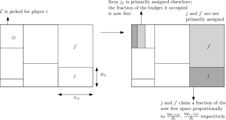
Figure 3: Consider on the left the above fractional assignment of configurations to player $i$; width corresponds to the assignment value of an item and height to its price. Here, $\mathcal{C}$ is picked for player $i$. Assuming all the items belong to $H$, every item in $\mathcal{C}$ has a constant probability of being assigned elsewhere; in this case, it was $j_{f}$. Then, every item which does not belong to $\mathcal{C}$ is secondarily assigned to $i$ with constant probability(in this case $j,j^{\prime}$) and claim a constant fraction of the free space, thus increasing its contribution to the objective value.

∎

We are now ready to prove Theorem 4. By Corollary 2 we are able to achieve a better than $\frac{3}{4}$ approximation guarantee when all items belong to $I$. The fractional assignments of items in $I$ are away from $\frac{1}{2}$ and therefore primary assignment is sufficient to return better than $3/4$-fraction of their contribution to the objective value. On the other hand, we get approximation guarantee greater than $\frac{3}{4}$ if all items belong to $H$ due to Lemma 11. The remaining scenario is when we have items from both $H$ and $I$.

Proof of Theorem 4.

By definition,

$$\mathsf{Val}(x^{*})=\sum_{j\in\mathcal{Q}}\mathsf{Val}_{j}(x^{*})=\sum_{j\in I}\mathsf{Val}_{j}(x^{*})+\sum_{j\in H}\mathsf{Val}_{j}(x^{*})$$

Now, remember that $j\in H$ is primarily assigned with probability $1-x_{ij}+x_{ij}^{2}$ and secondarily assigned with probability $x_{ij}(1-x_{ij})\geq\delta(1-\delta)$, where $i$ is one of the two players it can be assigned to. Let $s(j)$ be the player $j$ is secondarily assigned to when needed, and let $\rho_{j}=x_{s(j)j}$. From Lemmas 10 and 11 we have

$$\mathbb{E}[\mathsf{Val}(x^{*})]\geq\sum_{i\in\mathcal{A}}\sum_{j\in I}(1-\delta+\delta^{2})\mathsf{Val}_{ij}(y)+$$

$$\sum_{j\in H}(1-\rho_{j}(1-\rho_{j}))\mathsf{Val}_{j}(y)+\frac{\rho_{j}(1-\rho_{j})\mathsf{Val}_{j}(y)}{\sum_{\mathcal{C}\subseteq\mathcal{Q}:j\notin\mathcal{C}}y_{s(j)\mathcal{C}}}\sum_{\mathcal{C}\subseteq\mathcal{Q}:j\notin\mathcal{C}}y_{s(j)\mathcal{C}}\frac{\delta(1-\delta)}{2B_{s(j)}}\sum_{j^{\prime}\in\mathcal{C}\cap H}p_{s(j)j^{\prime}\mathcal{C}}=$$

$$\sum_{i\in\mathcal{A}}\sum_{j\in I}(1-\delta+\delta^{2})\mathsf{Val}_{ij}(y)+\sum_{j\in H}\frac{3}{4}\mathsf{Val}_{j}(y)+\rho_{j}\mathsf{Val}_{j}(y)\sum_{\mathcal{C}\subseteq\mathcal{Q}:j\notin\mathcal{C}}y_{s(j)\mathcal{C}}\frac{\delta(1-\delta)}{2B_{s(j)}}\sum_{j^{\prime}\in\mathcal{C}\cap H}p_{s(j)j^{\prime}\mathcal{C}}$$

Let $\lambda=\delta(1-\delta)$; the sum corresponding to items in $H$ now becomes

$$\sum_{j\in H}\frac{3}{4}\mathsf{Val}_{j}(y)+\frac{\rho_{j}\mathsf{Val}_{j}(y)\lambda}{2B_{s(j)}}\sum_{\mathcal{C}\subseteq\mathcal{Q}:j\notin\mathcal{C}}y_{s(j)\mathcal{C}}\left(\sum_{j^{\prime}\in\mathcal{C}}p_{s(j)j^{\prime}\mathcal{C}}-\sum_{j^{\prime}\in\mathcal{C}\cap I}p_{s(j)j^{\prime}\mathcal{C}}\right)$$

Our next goal will be to cancel out the negative term in the above sum; in order to do this, we will manipulate the sum corresponding to items in $I$ as follows: for all $i\in\mathcal{A}$, $j\in I$ we will remove a quantity equal to $\lambda\mathsf{Val}_{ij}(y)$ from the sum corresponding to items in $I$ and distribute it to items $j^{\prime}\in H$ which are assigned to $i$ in configuration $\mathcal{C}$ with a coefficient of $p_{ij\mathcal{C}}y_{i\mathcal{C}}$. So, the sum over almost-integral items becomes

$$\sum_{i\in\mathcal{A}}\sum_{j\in I}(1-\delta+\delta^{2}-\lambda)\mathsf{Val}_{ij}(y)$$

which means that choosing the right $\delta$ we will still be able to recover more than $\frac{3}{4}$ of the value of every item in $I$. On the other hand, because of this redistribution, we can consider that for any player $i$ the total subtracted value from items in $I$ is distributed to items assigned in $i$ proportionally to their fractional assignment; hence, we can actually consider that this quantity is distributed among configurations proportionally to their assignment and afterwards distributed among items in that configuration. In other words, for every item $j\in H$ and every configuration $\mathcal{C}$ that $j$ belongs to in $s(j)$, and every $j^{\prime}\in\mathcal{C}\cap I$, we will remove a $\lambda$ fraction of $y_{s(j)\mathcal{C}}p_{s(j)j^{\prime}\mathcal{C}}$(i.e. the contribution of $j^{\prime}$ to the objective value due to $\mathcal{C}$) and assign a $\frac{\mathsf{Val}_{s(j)j}(y)}{B_{s(j)}}$ fraction of it towards $j$. Hence, since $\mathsf{Val}_{s(j)j}(y)\geq\frac{\mathsf{Val}_{j}(y)}{2}$, the sum over items in $H$ becomes

$$\sum_{j\in H}\frac{3}{4}\mathsf{Val}_{j}(y)+\frac{\rho_{j}\mathsf{Val}_{j}(y)\lambda}{2B_{s(j)}}\sum_{\mathcal{C}\subseteq\mathcal{Q}:j\notin\mathcal{C}}y_{s(j)\mathcal{C}}\sum_{j^{\prime}\in\mathcal{C}}p_{s(j)j^{\prime}\mathcal{C}}$$

Since if there is a configuration which does not contain items of total value at least the budget of the corresponding player, our algorithm can only perform better (there is more leftover space than that which we have estimated), we can assume without loss of generality that for all $\mathcal{C}\subseteq\mathcal{Q}$ for which there is a player $i$ such that $y_{i\mathcal{C}}>0$, it holds $\sum_{j\in\mathcal{C}}p_{ij\mathcal{C}}=B_{i}$. Hence, the sum over items in $H$ becomes

$$\sum_{j\in H}\frac{3}{4}\mathsf{Val}_{j}(y)+\frac{\rho_{j}\mathsf{Val}_{j}(y)\lambda}{2}\sum_{\mathcal{C}\subseteq\mathcal{Q}:j\notin\mathcal{C}}y_{s(j)\mathcal{C}}=\sum_{j\in H}\frac{3}{4}\mathsf{Val}_{j}(y)+\frac{\rho_{j}(1-\rho_{j})\mathsf{Val}_{j}(y)\lambda}{2}\geq$$

$$\sum_{j\in H}\frac{3}{4}\mathsf{Val}_{j}(y)+\frac{\delta(1-\delta)\mathsf{Val}_{j}(y)\lambda}{2}$$

In total we have:

$$\mathbb{E}[\mathsf{Val}(x^{*})]\geq\sum_{i\in\mathcal{A}}\sum_{j\in I}(1-\delta+\delta^{2}-\lambda)\mathsf{Val}_{ij}(y)+\sum_{j\in H}\frac{3}{4}\mathsf{Val}_{j}(y)+\frac{\lambda\delta(1-\delta)}{2}\mathsf{Val}_{j}(y)=$$

$$\sum_{j\in I}(1-\delta+\delta^{2}-\lambda)\mathsf{Val}_{j}(y)+\sum_{j\in H}\frac{3}{4}\mathsf{Val}_{j}(y)+\lambda\delta(1-\delta)\mathsf{Val}_{j}(y)$$

Selecting $\delta$ such that $(1-\delta+\delta^{2}-\lambda)=(1-\delta+\delta^{2}-\delta(1-\delta))>\frac{3}{4}$, the theorem follows. ∎

7 An improved integrality gap for the unrestricted case

The previously best known upper bound on integrality gap of the configuration LP was $5/6=0.833$ proved by Chakrabarty and Goel in [5]. We improve this to $0.828$. Unlike the previous result, our gap instance is not a graph instance.

Theorem 5.

The integrality gap of the configuration LP is at most $2(\sqrt{2}-1)\approx 0.828$.

Proof.

For $p,q\in\mathbb{N}$ such that $p<q$, consider the following budget assignment instance: there are $q$ players $b_{i}\in B$ for $1\leq i\leq q$ with budget 1 and $q$ players $s_{i}\in S$ for $1\leq i\leq q$ with budget $\frac{p}{q}$. Additionally, there are $p$ items $c_{j}\in C$ for $1\leq j\leq p$, each of which can be assigned to players in $B$ with a value of 1. Finally, for each player $b_{i}\in B$, there are $q$ items $o_{i,j}\in O_{i}$ for $1\leq j\leq q$, which can be assigned to $b_{i}$ and $s_{i}$ with a value of $\frac{1}{q}$.

An example with $p=2$ and $q=3$ is drawn in Figure 4.

Figure 4: An instance with $p=2$ and $q=3$. Black squares are players in $B$, white squares players in $S$. They have budgets $1$ and $2/3$ respectively. Items in $C$ are black dots and items in $O_{i}$ are white dots with their values written next to them. An edge between a player and an item denotes that the player is interested in that item.

The optimal integral solution assigns $p$ items from $C$ to $p$ distinct players in $B$; for each player $i$ that is assigned an item from $C$, we assign $p$ items from $O_{i}$ to $s_{i}$. Let $i^{\prime}$ be one of the $q-p$ players which do not get an item from $C$, the optimal integral solution assigns the $q$ items from $\bigcup_{i=1}^{q}O_{i}$ to $i^{\prime}$. The total value of the solution is $p(1+\frac{p}{q})+q-p$.

Consider the following fractional solution to the configuration LP. Every item in $C$ is shared by the $q$ players in $B$, each with a fraction of $\frac{1}{q}$. Furthermore, every player $i$ in $B$ is assigned a fraction $\frac{q-p}{q}$ of every item in $O_{i}$. More precisely, the configuration $\mathcal{C}=O_{i}$ has $y_{i\mathcal{C}}=\frac{q-p}{q}$, so the budget of $i$ is completely filled.

Finally, every player $i$ in $S$ uses the unassigned fraction $\frac{p}{q}$ of every item in $O_{i}$ to form $p\choose q$ configurations of size $\frac{p}{q}$, which fill up the budget of $i$ completely. Hence, the value of the fractional solution is $q+q\frac{p}{q}=q+p$. Note that the total value of items is $p+q$, so there can not be a better assignment.

Hence, the integrality gap $I(p,q)$ is

$$I(p,q)=\frac{p(1+\frac{p}{q})+q-p}{p+q}=\frac{p^{2}+q^{2}}{q^{2}+pq}=\frac{\frac{p^{2}}{q^{2}}+1}{\frac{p}{q}+1}.$$

For $x\in\mathbb{R}$, the expression $f(x)=\frac{x^{2}+1}{x+1}$ is minimized at $x^{*}=\sqrt{2}-1$ and has $f(x^{*})=2(\sqrt{2}-1)$. Hence, choosing $p,q$ such that $\frac{p}{q}$ is arbitrarily close to $\sqrt{2}-1$, we can achieve an integrality gap arbitrarily close to $2(\sqrt{2}-1)$. ∎

8 Hardness of Approximation

In this section we strengthen the known hardness results. First we prove that the known $15/16$-hardness holds also for restricted MBA where players have the same budget and then we prove hardness $59/60$ in the graph case.

Theorem 6.

For every $\epsilon>0$, it is NP-hard to approximate restricted MBA within a factor of $15/16+\epsilon$. Furthermore, this is true for instances where all items can be assigned to at most 3 players and all players have the same budget.

Proof.

Chakrabarty and Goel in [5] prove the $(15/16+\epsilon)$-hardness for restricted MBA instances where all items can be assigned to at most 3 players. They achieve this by reducing Max-3-Lin(2)problem to MBA. The Max-3-Lin(2)problem was proved to be NP-hard to approximate within a factor of $1/2+\epsilon$ by Håstad in [12].

We use the same proof but use a different starting point. The result of Håstad can be modified with the technique of Trevisan [18] so that each variable in the Max-3-Lin(2)instance has the same degree.

The construction of Chakrabarty and Goel gives budget $4\deg(x)$ to the 2 players corresponding to variable $x$. Hence, if all variables have the same degree, all players have the same budget. ∎

Next, we modify the construction of Chakrabarty and Goel for use with linear equations of size 2. The important change is that we create items for assignments that do not satisfy an equation, while previous construction used satisfying assignments. The use of equations of size $2$ implies a hardness for the graph case, i.e. where each item can only be assigned to two players.

Theorem 7.

For every $\epsilon>0$, it is NP-hard to approximate graph MBA within a factor of $59/60+\epsilon$. Furthermore, this is true for the restricted instances where all players have the same budget.

Proof.

We reduce from an instance $\phi$ of Max-2-Lin(2). Let $x$ be a variable occurring $\deg(x)$ times in $\phi$. We have two players $\left<x:1\right>$ and $\left<x:0\right>$ both with budgets $\deg(x)$ and an item of value $\deg(x)$ that can only be assigned to these two players. The meaning of this item is that if it is assigned to the player $\left<x:a\right>$, then a truth assignment $\alpha$ has $\alpha(x)=a$.

For each equation $x+y=b$, there are two items $\left<x:a_{1},y:a_{2}\right>$ of value $1$. Each such item corresponds to an assignment $\alpha$ for which $\alpha(x)=a_{1},\alpha(y)=a_{2}$ and $a_{1}+a_{2}\not=b$. An item $\left<x:a_{1},y:a_{2}\right>$ can be assigned to $\left<x:a\right>$ and $\left<y:c\right>$ only if $a=a_{1}$ and $c=a_{2}$ respectively.

Every item can only be assigned to two players, so this is a graph instance. Furthermore, the valuation for both players is the same, so it is the restricted case.

The analysis is now very similar to the one in [5]. We can prove that an optimal assignment of items always assigns items of weight $\deg(x)$ and this can be translated into a truth assignment $\alpha$ to variables. We have $\alpha(x)=a$ if an item of value $\deg(x)$ is assigned to $\left<x:a\right>$. If $\alpha$ satisfies $x+y=b$, i.e. $\alpha(x)+\alpha(y)=b$, we can assign both items $\left<x:a_{1},y:a_{2}\right>$. Otherwise we can only assign one of them, since both $\left<x:\alpha(x)\right>$ and $\left<y:\alpha(y)\right>$ are fully assigned. So if $\phi$ is $\delta$-satisfiable with $m$ equations, the MBA instance has objective value $\sum_{x}\deg(x)+m(2\delta+(1-\delta))=3m+\delta m$.

Håstad and Trevisan et al. in [12] and [19] proved that it is NP-hard to distinguish instances of Max-2-Lin(2)that are at least $(3/4-\epsilon)$-satisfiable and those that are at most $(11/16+\epsilon)$-satisfiable. Hence it is hard to distinguish between an instance of MBA with objective value at least $3m+\frac{3}{4}m-\epsilon m=m(60/16-\epsilon)$ and at most $3m+\frac{11}{16}m+\epsilon m=m(59/16+\epsilon)$, where $m$ is the number of equations in $\phi$.

Therefore graph MBA is NP-hard to approximate to within a factor of $59/60+\epsilon$. The instance from [19] can also be modified to be regular, i.e. with all degrees $\deg(x)$ the same, thus producing an instance with equal budgets. This can be done by splitting each variable into more variables, as in [18]. ∎

9 Conclusion and future directions

We showed that the integrality gap for configuration LP is strictly better than $\frac{3}{4}$ for two interesting and natural restrictions of Maximum Budgeted Allocation: restricted and graph MBA.

These results imply that the configuration LP is strictly better than the natural assignment LP and pose promising research directions. Specifically, our results on restricted MBA suggest that our limitations in rounding configuration LP solutions do not necessarily stem from the items being fractionally assigned to many players, while our results on graph MBA suggest that they do not necessarily stem from the items having non-uniform prices. Whether these limitations can simultaneously be overcome is left as an interesting open problem.

Finally, it would be interesting to see whether the techniques presented, and especially the exploitation of the big items structure, can be applied to other allocation problems with similar structural features as MBA (e.g. GAP).

References

- [1] N. Andelman and Y. Mansour. Auctions with budget constraints. In SWAT, pages 26–38, 2004.
- [2] A. Asadpour, U. Feige, and A. Saberi. Santa claus meets hypergraph matchings. In APPROX–RANDOM, pages 10–20. Springer, 2008.
- [3] Y. Azar, B. E. Birnbaum, A. R. Karlin, C. Mathieu, and C. T. Nguyen. Improved approximation algorithms for budgeted allocations. In ICALP (1), pages 186–197, 2008.
- [4] N. Bansal and M. Sviridenko. The santa claus problem. In J. M. Kleinberg, editor, STOC, pages 31–40. ACM, 2006.
- [5] D. Chakrabarty and G. Goel. On the approximability of budgeted allocations and improved lower bounds for submodular welfare maximization and gap. SIAM J. Comput., 39(6):2189–2211, 2010.
- [6] T. Ebenlendr, M. Krčál, and J. Sgall. Graph balancing: A special case of scheduling unrelated parallel machines. In SODA, pages 483–490. Society for Industrial and Applied Mathematics, 2008.
- [7] U. Feige. On allocations that maximize fairness. In SODA, pages 287–293. SIAM, 2008.
- [8] U. Feige and J. Vondrák. Approximation algorithms for allocation problems: Improving the factor of 1 - 1/e. In FOCS, pages 667–676, 2006.
- [9] R. Gandhi, S. Khuller, S. Parthasarathy, and A. Srinivasan. Dependent rounding and its applications to approximation algorithms. J. ACM, 53(3):324–360, 2006.
- [10] R. Garg, V. Kumar, and V. Pandit. Approximation algorithms for budget-constrained auctions. In APPROX–RANDOM, pages 102–113. Springer, 2001.
- [11] M. Grötschel, L. Lovász, and A. Schrijver. Geometric Algorithms and Combinatorial Optimization, volume 2 of Algorithms and Combinatorics. Springer, 1993.
- [12] J. Håstad. Some optimal inapproximability results. J. ACM, 48(4):798–859, 2001.
- [13] B. Lehmann, D. J. Lehmann, and N. Nisan. Combinatorial auctions with decreasing marginal utilities. Games and Economic Behavior, 55(2):270–296, 2006.
- [14] J. K. Lenstra, D. B. Shmoys, and É. Tardos. Approximation algorithms for scheduling unrelated parallel machines. Math. Program., 46:259–271, 1990.
- [15] D. B. Shmoys and É. Tardos. An approximation algorithm for the generalized assignment problem. Math. Program., 62:461–474, 1993.
- [16] A. Srinivasan. Budgeted allocations in the full-information setting. In APPROX-RANDOM, pages 247–253, 2008.
- [17] O. Svensson. Santa claus schedules jobs on unrelated machines. SIAM J. Comput., 41(5):1318–1341, 2012.
- [18] L. Trevisan. Non-approximability results for optimization problems on bounded degree instances. In STOC, pages 453–461, 2001.
- [19] L. Trevisan, G. B. Sorkin, M. Sudan, and D. P. Williamson. Gadgets, approximation, and linear programming. SIAM J. Comput., 29(6):2074–2097, 2000.
- [20] J. Verschae and A. Wiese. On the configuration-LP for scheduling on unrelated machines. In Algorithms–ESA, pages 530–542. Springer, 2011.