Triple vector boson production through Higgs-Strahlung with NLO multijet merging

Abstract

Triple gauge boson hadroproduction, in particular the production of three $W$-bosons at the LHC, is considered at next-to leading order accuracy in QCD. The NLO matrix elements are combined with parton showers. Multijet merging is invoked such that NLO matrix elements with one additional jet are also included. The studies here incorporate both the signal and all relevant backgrounds for $VH$ production with the subsequent decay of the Higgs boson into $W$– or $\tau$–pairs. They have been performed using S HERPA +O PEN L OOPS in combination with C OLLIER .

1 Introduction

The imminent second round of data taking at the LHC presents new opportunities for studying physics at the electroweak to TeV scale. In light of the recent discovery of a Higgs boson [1, 2], with all experimental determinations of its properties up to now compatible with Standard Model expectations based on the Brout–Englert–Higgs (BEH) mechanism [3, 4, 5, 6], it is clear that increasingly precise studies become necessary in order to look for subtle effects where new physics could manifest itself.

A prime candidate for such studies is the production of multiple gauge bosons: channels involving $ZZ$, $WW$ and $\gamma\gamma$ final states have been employed, among others, for the discovery of the Higgs boson, while processes with $W\gamma$, $WZ$, $ZZ$, and $Z\gamma$ final states are frequently used by the experiments to search for anomalous triple gauge boson couplings, see for instance [7, 8, 9, 10]. Clearly, with higher energies, such searches can and will be extended to also include anomalous quartic gauge couplings. In addition, multi-boson channels, and in particular those that lead to final states involving three leptons, are important backgrounds in searches for new particles; as illustrative example consider neutralino-chargino pair production and their subsequent decay in supersymmetric extensions of the Standard Model.

This publication focuses on the production of a Standard Model Higgs boson in the Higgsstrahlung process (associated $VH$ production) and its subsequent decay into $W$– or $\tau$–pairs. Apart from the signal, all relevant background channels will be studied as well. This includes multiple gauge bosons final states such as $WZ$, $WWW$, $ZWW$, $ZZ$, $WZZ$ and $ZZZ$. The studies presented here follow closely the recent analyses by ATLAS and CMS [11, 12, 13].

In many of these processes, QCD corrections play a significant role, from highly phase-space dependent $K$-factors ranging between 1.5 and 2 to the fact that the emergence of additional jets can be used to shed light on the actual production mechanism giving rise to triple gauge boson final states. In addition, quite often vetoing additional jets is a very good way to suppress unwanted backgrounds, a prime example being the massive suppression of the $t_{\to W^{+}b}\bar{t}_{\to W^{-}\bar{b}}W$ background to $WWW$ production or other signals, which allows us here to ignore this class of processes.

For the signal process, $VH$–associated production, parton–level results are available at next-to leading order accuracy (NLO) in the perturbative expansion of QCD [14] and NNLO results are known for more than a decade [15, 16]. Resummed predictions were computed more recently [17]. The NLO QCD corrections to triple gauge boson production have first been calculated in [18, 19], the leptonic decay of the bosons has been discussed in [20, 21] and it has also been implemented in the V BF N LO code [22]. Predictions at NLO QCD for triple gauge boson production in association with one extra jet are presented for the first time in this paper.

For the calculation of the virtual corrections we employ O PEN L OOPS  [23], a fully automated one-loop generator based on a fast numerical recursion for multi-particle processes. For tensor and scalar integrals we use the C OLLIER library [24], which guarantees high numerical stability thanks to the methods of [25, 26, 27]. For the Born and real emission contributions the matrix element generators A MEGIC++  [28] and C OMIX  [29] are used. The mutual cancellation of infrared divergences in real and virtual contributions is achieved through the dipole formalism [30, 31] and its automated implementation in both A MEGIC++  [32] and C OMIX . The overall event generation is handled by S HERPA  [33, 34]. For the first time, the NLO QCD calculations are combined consistently with parton showers, employing the S–M C @N LO variant [35, 36] of M C @N LO  [37, 38]. Parton showers are generated by S HERPA , based on Catani–Seymour dipole subtraction [30, 31] as suggested in [39] and implemented in [40]. This setup for the matching was recently employed $W\!+3$ jets production [36], dijet production [41], and for $t\bar{t}b\bar{b}$ production in [42]. In addition, a multijet merging with NLO matrix elements including one additional jet is included, following the M E P S @N LO algorithm [43, 44]. This method has recently been employed for a number of processes, among them top pair production with up to two jets [45, 46], Higgs production in gluon fusion with up to two jets [47] and, similarly, the production of $4$ leptons in association with up to one jet [48].

The Monte-Carlo methods used to simulate jet production and evolution are discussed in Sec. 2. Section 3 presents results obtained with the S–M C @N LO matching and M E P S @N LO merging methods. We focus on the treatment of signal and background with typical cuts as used by ATLAS and CMS, [11, 12, 13]. This publication closes with a summary and some outlook in Section 4.

2 Matching and merging techniques in S HERPA

This section reviews the basic MC event generation techniques used in our analysis. We focus on new developments in matching and merging methods, which allow to combine fixed-order NLO calculations and parton shower simulations.

2.1 S–M C @N LO

Leading order cross sections, including the subsequent parton shower evolution in the initial and final state can schematically be written as

$${\rm d}\sigma^{\rm(PS)}\,=\,{\rm d}\Phi_{B}\,\mathrm{B}_{n}(\Phi_{B})\,\mathcal{F}_{n}(\mu_{Q}^{2})\;,$$ (2.1)

where ${\rm d}\Phi_{B}$ denotes the phase space element for the Born–level kinematics and $\mathrm{B}_{n}(\Phi_{B})$ is the Born–level differential cross section with $n$ external partons, composed of the corresponding parton–level cross section at leading order, convoluted with the PDFs and multiplied with suitable symmetry and flux factors. The parton shower evolution of the $n$–parton configuration is encoded in the generating functional, $\mathcal{F}_{n}(\mu_{Q}^{2})$ with the resummation scale $\mu_{Q}$. This scale is a free parameter, entering in addition to the renormalization and factorization scales $\mu_{R}$ and $\mu_{F}$, and it may be chosen in a process–dependent way. At leading order, $\mu_{Q}=\mu_{F}$. The parton–shower generating functional is defined by splitting kernels $\mathrm{K}_{n}$, and the corresponding Sudakov form factor $\Delta_{n}(t^{\prime},t)\,=\,\exp\big{[}-\int_{t^{\prime}}^{\,t}\,{\rm d}\Phi_{1}\,\mathrm{K}_{n}(\Phi_{1})\big{]}$

$$\mathcal{F}_{n}(t)\,=\,\Delta_{n}(t_{c},t)\,+\,\int_{t_{c}}^{t}{\rm d}\Phi_{1}^{\prime}\,\mathrm{K}_{n}(\Phi_{1}^{\prime})\,\Delta_{n}(t^{\prime},t)\,\mathcal{F}_{n+1}(t^{\prime})\,,$$ (2.2)

The emission phase space is parametrized in terms of evolution parameter $t$, splitting variable $z$, and azimuthal angle $\phi$ as ${\rm d}\Phi_{1}\,=\,{\rm d}t\,{\rm d}z\,{\rm d}\phi\,J(t,z,\phi)$, where $J(t,z,\phi)$ denotes a Jacobian factor. $t_{c}$ is the infrared cut-off of the parton shower, typically of the order of a GeV. Equation (2.2) simultaneously describes the probability of no further parton emission (first term) and a single emission at scale $t^{\prime}$ (second term). If such an emission takes place, Eq. (2.2) is iterated, with the boundary conditions set by the newly formed partonic state.

By now, there are two different classes of algorithms to promote the leading order (LO) expression in Eq. (2.1) to NLO accuracy, namely the P OWHEG method [49, 50] and the M C @N LO matching method [37]. In M C @N LO , the parton-shower approximation is used to obtain universal subtraction terms that can be used to cancel the singularities in real and virtual corrections. This method was extended in [35, 36, 41] by modifying the parton shower such that its splitting kernels for the first emission include the full color and spin dependence present in the real corrections. This may introduce color–suppressed but logarithmically enhanced contributions into the Sudakov form factor. This method is referred to as S–M C @N LO in the following. Its cross section is computed as

$${\rm d}\sigma^{\text{(S--M\scalebox{0.8}{C}@N\scalebox{0.8}{LO})}}\,=\;{\rm d}\Phi_{B}\,\bar{\mathrm{B}}_{n}(\Phi_{B})\,\bar{\mathcal{F}}_{n}(\mu_{Q}^{2})\,+\,{\rm d}\Phi_{R}\,\mathrm{H}_{n}(\Phi_{R})\,\mathcal{F}_{n+1}(\tilde{\mu}_{Q}^{2})\;,$$ (2.3)

where the combination of $\bar{\mathrm{B}}$ and $\mathrm{H}$ provides the exact next-to leading order cross section and the functionals $\mathcal{F}_{n}$ and $\bar{\mathcal{F}}_{n}$ change its phase-space dependence, but not the normalization. $\mathrm{H}_{n}$ captures the subtracted real-emission contribution, while $\bar{\mathrm{B}}_{n}$ contains all other terms, projected onto Born kinematics.

$$\begin{split}\bar{\mathrm{B}}_{n}(\Phi_{B})\,=&\;\mathrm{B}_{n}(\Phi_{B})+\tilde{\mathrm{V}}_{n}(\Phi_{B})+\mathrm{I}_{n}(\Phi_{B},\,\mu_{Q}^{2})\,,\\ \mathrm{H}_{n}(\Phi_{R})\,=&\;\mathrm{R}_{n}(\Phi_{R})-\mathrm{D}_{n}(\Phi_{R})\,\Theta\left(\mu_{Q}^{2}-t\right)\;.\end{split}$$ (2.4)

In addition to the squared Born matrix element $\mathrm{B}_{n}(\Phi_{B})$ the virtual and real corrections, $\tilde{\mathrm{V}}_{n}(\Phi_{B})$ and $\mathrm{R}_{n}(\Phi_{R})$ respectively, have been introduced, the latter together with the corresponding phase space element ${\rm d}\Phi_{R}$. This phase space element factorizes as $\Phi_{R}\,=\,\Phi_{B}\times\Phi_{1}$, which is used to facilitate integration of the subtraction terms $\mathrm{D}_{n}(\Phi_{B},\Phi_{1})$ over the one–particle emission phase space and define the integrated subtraction terms $\mathrm{I}_{n}(\Phi_{B})$ [30, 31],

$$\mathrm{I}_{n}(\Phi_{B},\,\mu_{Q}^{2})\,=\,\int{\rm d}\Phi_{1}\,\mathrm{D}_{n}(\Phi_{B},\Phi_{1})\,\Theta\left(\mu_{Q}^{2}-t\right)\;.$$ (2.5)

Equation (2.5) is known analytically in $d$ dimensions for $\mu_{Q}^{2}\to\infty$, as is necessary to extract the poles in the dimensional regularization parameter $\varepsilon$. The value for finite $\mu_{Q}^{2}$ is computed by calculating the finite remainder in $d=4$ dimensions with Monte-Carlo techniques [36, 41].

The generating functional of the S–M C @N LO is defined as

$$\bar{\mathcal{F}}_{n}(t)\,=\;\bar{\Delta}_{n}(t_{c},t)\,+\,\int_{t_{c}}^{t}\!{\rm d}\Phi_{1}^{\prime}\,\frac{\mathrm{D}_{n}(\Phi_{B},\Phi_{1}^{\prime})}{\mathrm{B}_{n}(\Phi_{B})}\,\bar{\Delta}_{n}(t^{\prime},t)\,\mathcal{F}_{n+1}(t^{\prime})\;.$$ (2.6)

It differs from the parton-shower expression, Eq. (2.2), by sub-leading color contributions and spin correlation effects. Note that all secondary emissions are treated by a standard parton shower, indicated by $\mathcal{F}_{n+1}(t^{\prime})$.

2.2 ME NLO PS

The method outlined above can be improved with higher-order tree-level calculations using a multi-jet merging technique [61, 62, 43]. A merging scale, $Q_{\text{cut}}$, is introduced, like in the pure LO merging algorithms [51, 52, 53, 54, 55, 56, 57], which restricts the phase space of emissions in the parton shower from above, and emissions in the matrix elements from below.

The restricted M C @N LO simulation for the “core” process with $n$ particles generates the following terms

$$\begin{split}{\rm d}\sigma_{n}^{\rm excl}\,=&\;{\rm d}\Phi_{n}\;\bar{\mathrm{B}}_{n}(\Phi_{n})\,\bar{\mathcal{F}}_{n}(\mu_{Q}^{2}\,;<\!Q_{\rm cut})\\ &{}+{\rm d}\Phi_{n+1}\,\Theta(Q_{\rm cut}-Q(\Phi_{n+1}))\,\mathrm{H}_{n}(\Phi_{n+1})\,\mathcal{F}_{n+1}(\mu_{Q}^{2}\,;<\!Q_{\rm cut})\;,\end{split}$$ (2.7)

where $\bar{\mathcal{F}}_{n}(\mu_{Q}^{2}\,;<\!Q_{\rm cut})$ is the functional of the vetoed S–M C @N LO , and $\mathcal{F}_{n+1}(\mu_{Q}^{2}\,;<\!Q_{\rm cut})$ is the functional of the truncated vetoed parton shower [49, 50, 57].

The next higher jet multiplicities are calculated at leading order accuracy. A local $K$-factor is applied to preserve the total cross section to NLO accuracy,

$$\begin{split}{\rm d}\sigma_{n+k}\,=&\;{\rm d}\Phi_{n+k}\,\Theta(Q(\Phi_{n+k})-Q_{\rm cut})\;k_{n}\!\left(\Phi_{n+1}(\Phi_{n+k})\right)\;\mathrm{B}_{n+k}(\Phi_{n+k})\;\mathcal{F}_{n+k}(\mu_{Q}^{2}\,;<\!Q_{\rm cut})\;.\end{split}$$ (2.8)

Here $\Phi_{n+1}(\Phi_{n+k})$ is defined by the kinematics mapping of the parton shower, and

$$\begin{split}k_{n}(\Phi_{n+1})\,=\;\frac{\bar{\rm B}_{n}(\Phi_{n})}{{\rm B}_{n}(\Phi_{n})}\left(1-\frac{\mathrm{H}_{n}(\Phi_{n+1})}{{\rm R}_{n}(\Phi_{n+1})}\right)+\frac{\mathrm{H}_{n}(\Phi_{n+1})}{{\rm R}_{n}(\Phi_{n+1})}\;.\end{split}$$ (2.9)

is the local $K$-factor [43]. It is constructed such that a sample where exactly one jet at leading order accuracy is merged on top of the underlying S–M C @N LO reproduces this S–M C @N LO except for potential sub-leading color corrections in the S–M C @N LO $n$-jet simulation versus the showered $n+1$-jet simulation.

2.3 M E P S @N LO

The above merging method can be extended to the next-to-leading order also for the $n+k$-jet exclusive simulations. In order not to spoil the NLO-accuracy of these simulations it is not enough to simply implement a truncated vetoed parton shower as this is done in leading-order merging. The first-order expansion of the vetoed shower would generate corrections of order $\alpha_{s}$, which must be subtracted. This leads to the following expression for the differential cross section in the $n+k$-jet sample:

$$\begin{split}{\rm d}\sigma_{n+k}^{\rm excl}\,=&\;{\rm d}\Phi_{n+k}\,\Theta(Q(\Phi_{n+k})-Q_{\rm cut})\;\tilde{\mathrm{B}}_{n+k}(\Phi_{n}+k)\,\bar{\mathcal{F}}_{n+k}(\mu_{Q}^{2}\,;<\!Q_{\rm cut})\\ &+{\rm d}\Phi_{n+k+1}\,\Theta(Q(\Phi_{n+k})-Q_{\rm cut})\,\Theta(Q_{\rm cut}-Q(\Phi_{n+k+1}))\,\tilde{\mathrm{H}}_{n+k}(\Phi_{n+k+1})\,\mathcal{F}_{n+k+1}(\mu_{Q}^{2}\,;<\!Q_{\rm cut})\;,\end{split}$$ (2.10)

The extended subtraction is implemented by the modified differential cross sections $\tilde{\mathrm{B}}_{n+k}(\Phi_{n+k})$ and $\tilde{\mathrm{H}}_{n+k}(\Phi_{n+k+1})$, defined as

$$\begin{split}\tilde{\rm B}_{i}(\Phi_{i})=&\;{\rm B}_{i}(\Phi_{i})+\tilde{\mathrm{V}}_{i}(\Phi_{i})+{\rm I}_{i}(\Phi_{i})+\int{\rm d}\Phi_{1}\,\left[\tilde{\rm D}_{i}(\Phi_{i},\Phi_{1})-{\rm D}_{i}(\Phi_{i},\Phi_{1})\right]\\ \tilde{\mathrm{H}}_{i}(\Phi_{i+1})=&\;\mathrm{R}_{i}(\Phi_{i+1})-\tilde{\mathrm{D}}_{i}(\Phi_{i+1})\;,\\ \end{split}$$ (2.11)

which take the probability of truncated parton shower emissions into account [44, 43]. To this end, the dipole terms used in the S–M C @N LO are extended by the parton-shower emission probabilities, $\mathrm{B}_{i}(\Phi_{i})\,\mathrm{K}_{j}(\Phi_{1,i+1})$, where $\mathrm{K}_{j}(\Phi_{1,i+1})$ is the sum of all shower splitting functions for the intermediate state with $j<i$ in a predefined shower tree which leads to the final state with kinematical configuration $\Phi_{i}$. Thus,

$$\tilde{\mathrm{D}}_{i}(\Phi_{i+1})\,=\;\mathrm{D}_{i}(\Phi_{i+1})\,\Theta(t_{i}-t_{i+1})\;+\sum_{j=0}^{i-1}\mathrm{B}_{i}(\Phi_{i})\,\mathrm{K}_{j}(\Phi_{1,i+1})\,\Theta(t_{j}-t_{i+1})\,\Theta(t_{i+1}-t_{j+1})\,\Big{|}_{\,t_{0}=\mu_{Q}^{2}}\;.$$ (2.12)

This expression has a simple physical interpretation: The first term corresponds to the coherent emission of a parton from the external $i$-parton final state. It contains all soft and collinear singularities which are present in the real-emission matrix elements. The sum in the second term corresponds to emissions from the intermediate states with $i$ partons and in fact the terms $\mathrm{B}_{i}(\Phi_{i})\,\mathrm{K}_{j}(\Phi_{1,i+1})$ stem from the expansion of the Sudakov form factor of the truncated shower to first order in the strong coupling. All these terms can be implemented in the parton shower approximation, because soft divergences are regulated by the finite mass of the intermediate particles.

3 Results

3.1 Details of the analyses

There are current efforts from both CMS and ATLAS to search for the trilepton ($\ell=e,\mu$) final states emerging from $WH$–associated production, where the Higgs boson decays either into $\tau$ or $W$ pairs [11, 12, 13]. These final states allow a direct probe of the coupling between the Higgs boson and the weak bosons. In the following we present two analyses: the first inspired by a recent search by the CMS collaboration [13], the second following searches from the ATLAS collaboration [11, 12]. The majority of the cuts that are applied in both are given in Tab. 1. Their crucial features in reducing unwanted backgrounds are a veto on $Z$ bosons, which is realized differently in both analysis, and vetoes on jet activity to eliminate the large background from $t\bar{t}V$ production. Jets are reconstructed in both analyses using the anti-$k_{T}$ algorithm [63, 64] with the parameters given in Tab. 1. In the ATLAS-inspired analysis, events are allowed to contain at most one jet, which must not be a $b$-jet. The CMS-inspired analysis vetoes all events with a jet of $p_{\perp}>40\,\mathrm{GeV}$ and any containing $b$-jets. Both analyses dress electrons with all surrounding photons within a cone of $\Delta R=0.1$ while muons are left bare.

The ATLAS-inspired analysis requires exactly three isolated leptons of net charge $\pm 1$. At least one of the leptons needs to have a transverse momentum of more than 25 GeV for electrons and 21 GeV for muons, the other two leptons $p_{\perp}>10\,\mathrm{GeV}$ each. They are labeled in the following way: the lepton with charge different from the others is called lepton 0, of the two others the one with smaller distance $\Delta R$ from lepton 0 is called lepton 1 and the remaining one is labeled as lepton 2. The leptons are considered isolated if the transverse energy of all visible particles in a cone of radius $\Delta R_{\text{iso}}=0.2$ for leptons 0 and 1 and $\Delta R_{\text{iso}}=0.4$ for lepton 2 around the lepton is less than 10 % of the lepton $p_{\perp}$. After this pre-selection events containing a same-flavor-opposite-sign (SFOS) lepton pair are classified as $Z$ enriched, those that do not belong to the $Z$ depleted sample. In this publication only the $Z$ depleted subsample is considered. Contrary to the experimental analysis in [12] no requirement on the missing transverse energy is applied.

The CMS-inspired analysis on the contrary requires at least three isolated leptons of net charge $\pm 1$. Of those, at least one is required to have $p_{\perp}>20\,\mathrm{GeV}$ while the others must only fulfil $p_{\perp}>10\,\mathrm{GeV}$. The lepton isolation in turn depends on lepton flavor rather than classification. Electrons are considered isolated if in a cone of radius $\Delta R_{\text{iso}}=0.4$ the sum of the transverse energy of all visible particles does not exceed 15 % of the lepton $p_{\perp}$, while muons must satisfy this limit only in a cone of size $\Delta R_{\text{iso}}=0.3$. In case a pair of same-flavor-opposite-sign (SFOS) leptons is present in the event, the event is discarded if its invariant mass is closer to the nominal $Z$ boson mass than 25 GeV.

Cut	ATLAS	CMS
$p_{\perp,\,{\mathrm{min}}}^{\ell}$	10 GeV	10 GeV
$|\eta^{e}_{\mathrm{max}}|$	2.47	2.5
$|\eta^{\mu}_{\mathrm{max}}|$	2.5	2.4
$N_{\mathrm{leptons}}$	3	$\geq$3
$Z$ veto	no SFOS	$|m_{Z}-m_{\mathrm{SFOS}}|>25\,\mathrm{GeV}$
$|\sum Q_{\ell}|$	$+1$	$+1$
Jet $p_{\perp,\mathrm{min}}$	25 GeV	20 GeV
Jet d$R$	0.4	0.5
$E_{\perp,\,\mathrm{min}}^{\mathrm{miss}}$	–	40 GeV

Table 1: Cuts for the ATLAS- and CMS-inspired analyses.

Both the ATLAS and CMS analyses include regions with more cuts than are described here, however the observables presented do not use these regions.

3.2 Monte Carlo samples

We consider $pp\to 3\ell+E_{\perp}^{\text{miss}}+X$ production at the LHC at a center-of-mass energy of 8 TeV. All processes with at least three leptons that involve an on–shell Higgs boson are considered as signal processes, and those which do not are considered background processes. Neutrinos do not necessarily need to be present as missing transverse energy can also be generated due to the limited detector acceptance in rapidity.

The signal is comprised primarily of $W^{\pm}H(\rightarrow W^{+}W^{-})$, $W^{\pm}H(\rightarrow\tau^{+}\tau^{-})$ and $ZH(\rightarrow W^{+}W^{-})$, but includes also $ZH(\rightarrow\tau^{+}\tau^{-})$, $W^{\pm}H(\rightarrow ZZ)$ and $ZH(\rightarrow ZZ)$ as subdominant contributions. All signal processes are calculated at M E P S @N LO accuracy, merging the respective processes accompanied by zero/one jets at NLO and by two jets at LO accuracy. The background processes considered are high multiplicity bosonic final states: $W^{\pm}Z$, $ZZ$, $W^{\pm}W^{+}W^{-}$, $W^{+}W^{-}Z$, $W^{\pm}ZZ$ and $ZZZ$, which can evade the $Z$ veto by the same method as $W^{\pm}Z$, and also include hadronic decays of the bosons. Higher multiplicity final states do not have a significant enough contribution to be considered. In addition, the production of an off–shell Higgs boson decaying to an on–shell $V$ boson pair is also considered as part of the background. The cross section for this process is very small as compared to the production of the on–shell Higgs boson, and it contributes mostly through its interference with the triple boson background. The $W^{\pm}Z$ boson background remains dominant over large portions of phase space; this is due to lost leptons and, more importantly, due to decays into $\tau$-leptons which enable the evasion of the $Z$ veto. Of less importance is the $W^{\pm}W^{+}W^{-}$ process, nonetheless warranting high theoretical accuracy. Thus, both $W^{\pm}Z$ and $W^{\pm}W^{+}W^{-}$ are calculated at the same accuracy as the signal processes, while the remaining subdominant background processes, $ZZ$, $W^{+}W^{-}Z$, $W^{\pm}ZZ$ and $ZZZ$, are considered at ME NLO PS accuracy, i.e. NLO accuracy for the respective inclusive process and leading order accuracy when the gauge bosons are accompanied by one and two jets. Further, in order to prevent $tV_{1}V_{2}$/$\bar{t}V_{1}V_{2}$ contributions entering the $V_{1}V_{2}W^{\pm}j$ calculation, and $t\bar{t}V$ contributions entering the $VW^{+}W^{-}jj$ calculation, only light quarks are considered in the matrix element final state.

The Higgs and $W/Z$ gauge boson decays are treated in the narrow width approximation, including spin correlation effects throughout all decay chains. The kinematics are then corrected by redistributing the boson’s propagator mass onto a Breit-Wigner distribution. In cases where $1\to 2$ decays are not allowed kinematically their $1\to 3$ substructure is resolved. This is relevant mainly for $H\to VV^{*}$ decays. Additionally, all decays receive higher-order QCD and QED corrections through intermediate parton showering or YFS-type soft-photon resummation (including full $\mathcal{O}(\alpha)$ corrections) [65], respectively. Throughout, all possible decays leading to the desired final state are considered, including all invisible $Z$- and hadronic $W$-, $Z$- and $\tau$-decay channels.

The distributions for the central values include hadronization [66] and an underlying event simulation [67]. The CT10 parton distributions [68] have been used throughout. Scales are set according to the CKKW prescription [57, 44] and the uncertainties are evaluated as follows

• To determine the renormalization scale the event is clustered using the inverse of the parton shower, including electroweak splitting functions as introduced in [69, 70], until a $2\to 2$ core configuration is reached. The renormalization scale $\mu_{R}$ is then defined through

  $$\alpha_{s}^{k+n}(\mu_{R})\;=\;\alpha_{s}^{k}(\mu_{\text{core}})\prod\limits_{i=1}^{n}\alpha_{s}(t_{i})\,,$$ (3.1)

  wherein $k$ is the QCD order of the such determined core process at tree level, i.e. $k=0$ for $q\bar{q}^{(\prime)}\to VV^{(\prime)}$ or $q\bar{q}^{(\prime)}\to VH$, $k=1$ for $q\bar{q}^{(\prime)}\to Vg$ or $gq\to Vq^{(\prime)}$, and $k=2$ for pure QCD core processes. $n$ is the final state clustered jet multiplicity and the $t_{i}$ their respective reconstructed emission scales. As core scale we choose $\mu_{\text{core}}=\hat{s}$ for $k=0$, $\mu_{\text{core}}=\tfrac{1}{2}\,m_{\perp}(V)$ for $k=1$, and $\mu_{\text{core}}=\tfrac{1}{2}\,p_{\perp}$ for $k=2$. For $n=k=0$ we set $\mu_{R}=\mu_{\text{core}}$. The factorization scale is set to $\mu_{F}=\mu_{\text{core}}$ on the core configuration. The thus determined $\mu_{R}$ and $\mu_{F}$ are then varied by a factor of 2.

• The resummation scale $\mu_{Q}$, also defined in [44], is set equal to the factorization scale. It is varied by a factor of $\sqrt{2}$, cf. [41, 47].

• $Q_{\rm cut}$ is the merging scale. Three values are chosen for this scale, 15 GeV, 30 GeV and 60 GeV.

The uncertainties in all figures are shown as two bands, one for the combined background and one for the combined signal, accumulated through their respective contributing processes only. They have been evaluated at the parton level. The full perturbative uncertainty for each process is obtained as the quadratic sum of the envelopes provided by the variation of the perturbative scales, $\mu_{R}$, $\mu_{F}$, and $\mu_{Q}$, and the merging scale $Q_{\rm cut}$. As non-perturbative uncertainties were found to be very small, these parton level uncertainties are directly applicable to the hadron level results. The electroweak input parameters for this simulation are $\alpha=1/128.802$, $m_{W}=80.419~{}\mathrm{GeV}$, $m_{Z}=91.188~{}\mathrm{GeV}$ and $m_{H}=125~{}\mathrm{GeV}$.

3.3 Results with M E P S @N LO

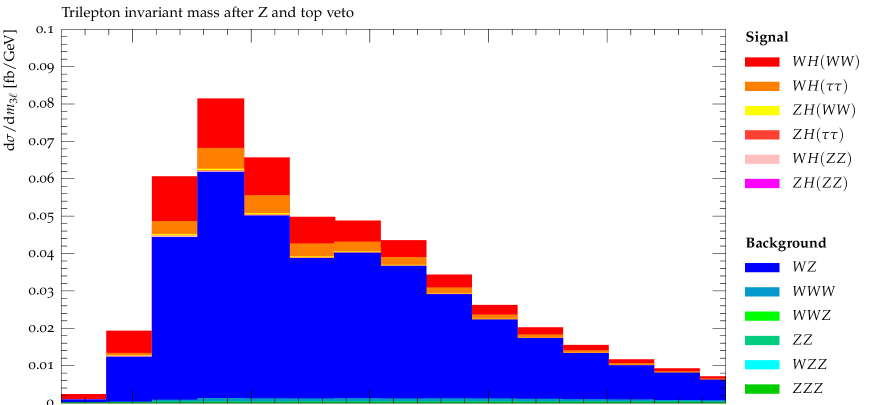
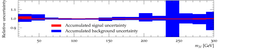
Figure 1: The trilepton invariant mass after CMS cuts. All contributing processes, grouped as whether considered signal or background, are added incoherently, ordered by relative contribution. The inset displays the same information on a logarithmic scale to better quantify the contributions of the rarer processes. Below the main plot the accumulated relative uncertainties originating from the respective signal and background processes to the total expected cross section are detailed.

This section presents selected observables defined on the event samples prepared with the analyses described in Sec. 3.1 applied to the calculations of Sec. 3.2. All observables considered below show a clear signal over background excess. They focus on the leptons from the hard process after the $Z$ and jet veto. The $Z$ veto is very important in these analyses, as without it the $W^{\pm}Z$ process is very dominant over both the signal and the background, while without the jet veto top associated vector boson production would bury the Higgs processes.

The first observable we consider is the trilepton invariant mass of events in the CMS-inspired analysis in Fig. 1. After the veto on the $Z$ boson and final state $b$-jets, the invariant mass distribution of the 3 leptons can be used to distinguish the signal from the background as a visible 30% excess is seen in the peak region, far surmounting the background uncertainties displayed in the lower panel. Very similar findings are made when looking at events in the ATLAS-inspired analysis. Although the main signal process $W^{\pm}H(W^{+}W^{-})$ forms the majority of the excess, the contribution from $W^{\pm}H(\tau\tau)$ is non-negligible, albeit of a slightly different shape. Regarding the background processes, the tri-boson processes have a significantly harder $m_{3\ell}$ spectrum, raising their relative contribution in the high-mass region, as can be seen in the logarithmically plotted inlay.

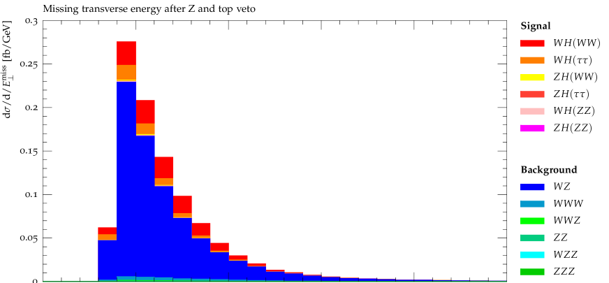
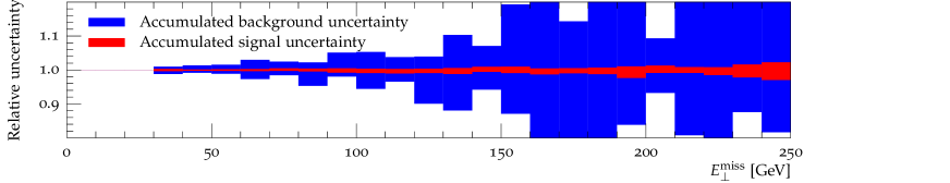
Figure 2: The missing transverse energy spectrum after CMS cuts. For details, see Fig. 1.

A somewhat complementary observable is the missing energy distribution, exhibited in Fig. 2, again effected on the event selection of the CMS-inspired analysis. The findings indeed display a similar behavior to the trilepton invariant mass distribution of Fig. 1, in that the signal is clearly visible above the background for $E_{\perp}^{\text{miss}}\lesssim 100\,\mathrm{GeV}$. Again, the dominant and subdominant signal processes, $W^{\pm}H(W^{+}W^{-})$ and $W^{\pm}H(\tau\tau)$, exhibit somewhat different shapes, with $W^{\pm}H(\tau\tau)$ possessing less missing transverse momentum. In both observables, the $W^{\pm}Z$ background is the most dominant background. However, here the di-boson and tri-boson background have a very similar behavior at large $E_{\perp}^{\text{miss}}$.

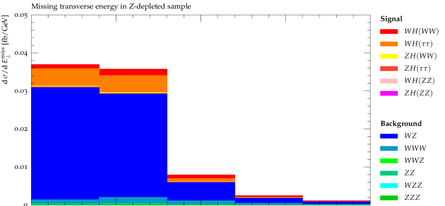
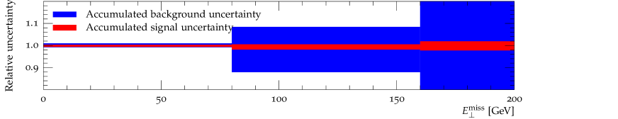
Figure 3: The missing transverse energy spectrum after ATLAS cuts. For details, see Fig. 1.

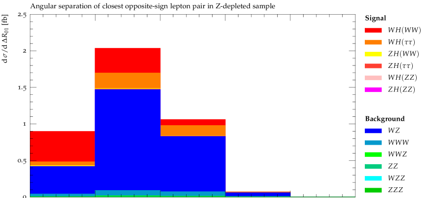
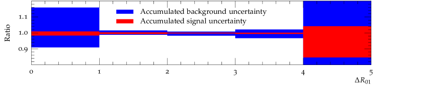
Figure 4: The angular separation of the closest pair of oppositely charged leptons in the case that no SFOS pair of leptons is found in the event after ATLAS cuts. For details, see Fig. 1.

The relatively small excess in the $E_{\perp}^{\text{miss}}$ spectrum in the CMS-inspired event selection is enhanced in the ATLAS-inspired event selection with its stronger $Z$ veto, implemented through a complete rejection on SFOS lepton pairs. Here, the $E_{\perp}^{\text{miss}}$ distribution shows an excess of the signal over the background of up to 50%. This is displayed in Fig. 3. In contrast to the case of a $Z$ veto through a mass window as in CMS, where the distribution especially for $W^{\pm}Z$ falls off smoothly, here the $Z$ veto introduces a visible kink, while the signal remains unaffected. This of course could be further used to reduce the $W^{\pm}Z$ background by utilizing this different impact on the respective shapes.

The angular separations between pairs of leptons are interesting observables for this process. Fig. 4 shows the distance $\Delta R$ between the closer of the two pairs of oppositely signed leptons, following the ATLAS-inspired event selection. These leptons do not have the same flavor, as this observable isolates the leptons that are most likely to be products of the Higgs boson decay to $W^{+}W^{-}$ or $\tau$ pairs. This effect in particular on the $WW$ channel stems from the spin correlations in the decay of the Higgs boson, as already discussed in [11]. As a result, this observable also has good discriminating power between signal and background, providing a clear excess in the region $\Delta R<3$. It also, better than the other observables considered, separates the two main signal processes. While $W^{\pm}H(W^{+}W^{-})$ constitutes approximately $80\,\mathrm{\%}$ of the Higgs signal below $\Delta R=1$, $W^{\pm}H(\tau\tau)$ contributes roughly $60\,\mathrm{\%}$ in the region $2<\Delta R<3$. There, however, the signal excess over the background has fallen from a factor of two to approximately $35\,\mathrm{\%}$ of the background expectation.

The different uncertainties have been investigated individually for all processes to check for their dominant source. In nearly all bins of all observables considered here, the uncertainties are driven by the renormalization and factorization scale variation with a typical effect on the few–percent level up to about 10% for the tri-boson processes. In regions dominated by jet activity of course the ME NLO PS samples, being at leading order accuracy only, exhibit a stronger dependence than those processes simulated with M E P S @N LO . In addition, it is worth stressing that effects due to hadronization and the underlying event are practically irrelevant for the uncertainties in the simulation of the processes for the observables considered here. Their main effect is on the isolation efficiency of the leptons. Although the non-perturbative corrections have a clear impact on the shape of trilepton invariant mass of Fig. 1, as the isolation is $p_{\perp}$-dependent, their uncertainties are barely noticeable. On the contrary, the missing transverse energies of Figs. 2 and 3 and the angular separation of Fig. 4 receive merely a change of the overall rate from effecting non-perturbative corrections. Again, their uncertainties are negligible.

4 Conclusions

In this publication NLO QCD accurate predictions for multiple weak boson production at the LHC were presented, and their application to Higgs boson searches based in trilepton final states has been highlighted. The $W^{\pm}H$ and $ZH$ Higgsstrahlung signals as well as the main backgrounds, $W^{\pm}Z$ and $W^{\pm}W^{+}W^{-}$ production, have been simulated at NLO including up to one extra jet in the M E P S @N LO multi-jet merging framework. The simulation of the $W^{\pm}W^{+}W^{-}$ background represents a nontrivial application of multi-jet merging at NLO and plays and important role for all Higgs and new-physics searches based on trilepton final states and jet vetoes. Also various other diboson and tribosons background processes have beed computed at NLO QCD, including matching to the parton shower and an improved description of extra jet radiation, based on the MENLOPS technique. We confirm, at NLO, that the relevant backgrounds to $W^{\pm}H$ and $ZH$ production are given by diboson and triboson production processes, if jet vetoes can be applied. We also show that the residual perturbative uncertainties in large fractions of the relevant phase space are of the order of 10% or even below. This will offer excellent opportunities for Higgs boson precision studies at the forthcoming LHC runs.

References

- [1] G. Aad et al., ATLAS Collaboration, Observation of a new particle in the search for the Standard Model Higgs boson with the ATLAS detector at the LHC, Phys.Lett. B716 (2012), 1–29, [arXiv:1207.7214 [hep-ex]].
- [2] S. Chatrchyan et al., CMS Collaboration, Observation of a new boson at a mass of 125 GeV with the CMS experiment at the LHC, Phys.Lett. B716 (2012), 30–61, [arXiv:1207.7235 [hep-ex]].
- [3] F. Englert and R. Brout, Broken Symmetry and the Mass of Gauge Vector Mesons, Phys.Rev.Lett. 13 (1964), 321–323.
- [4] P. W. Higgs, Broken symmetries, massless particles and gauge fields, Phys.Lett. 12 (1964), 132–133.
- [5] P. W. Higgs, Broken Symmetries and the Masses of Gauge Bosons, Phys.Rev.Lett. 13 (1964), 508–509.
- [6] G. Guralnik, C. Hagen and T. Kibble, Global Conservation Laws and Massless Particles, Phys.Rev.Lett. 13 (1964), 585–587.
- [7] G. Aad et al., ATLAS Collaboration, Measurement of the ZZ production cross section and limits on anomalous neutral triple gauge couplings in proton-proton collisions at sqrt(s) = 7 TeV with the ATLAS detector, Phys.Rev.Lett. 108 (2012), 041804, [arXiv:1110.5016 [hep-ex]].
- [8] G. Aad et al., ATLAS Collaboration, Measurement of the production cross section and limits on anomalous triple gauge couplings in proton-proton collisions at TeV with the ATLAS detector, Phys.Lett. B709 (2012), 341–357, [arXiv:1111.5570 [hep-ex]].
- [9] G. Aad et al., ATLAS Collaboration, Measurement of and production cross sections in collisions at TeV and limits on anomalous triple gauge couplings with the ATLAS detector, Phys.Lett. B717 (2012), 49–69, [arXiv:1205.2531 [hep-ex]].
- [10] S. Chatrchyan et al., CMS Collaboration, Measurement of the and inclusive cross sections in pp collisions at = 7 TeV and limits on anomalous triple gauge boson couplings, arXiv:1308.6832 [hep-ex].
- [11] ATLAS Collaboration, Search for associated production of the Higgs boson in the and channels with the ATLAS detector at the LHC, ATLAS–CONF–2013–075, ATLAS–COM–CONF–2013–069.
- [12] ATLAS Collaboration, Search for the Associated Higgs Boson Production in the Decay Mode Using 4.7 of Data Collected with the ATLAS Detector at TeV, ATLAS–CONF–2012–078, ATLAS–COM–CONF–2012–094.
- [13] CMS Collaboration, Search for SM Higgs in to to , CMS–PAS–HIG–13–009.
- [14] T. Han and S. Willenbrock, QCD correction to the and total cross-sections, Phys.Lett. B273 (1991), 167–172.
- [15] O. Brein, A. Djouadi and R. Harlander, NNLO QCD corrections to the Higgs-strahlung processes at hadron colliders, Phys.Lett. B579 (2004), 149–156, [arXiv:hep-ph/0307206 [hep-ph]].
- [16] G. Ferrera, M. Grazzini and F. Tramontano, Associated WH production at hadron colliders: a fully exclusive QCD calculation at NNLO, Phys.Rev.Lett. 107 (2011), 152003, [arXiv:1107.1164 [hep-ph]].
- [17] S. Dawson, T. Han, W. Lai, A. Leibovich and I. Lewis, Resummation Effects in Vector-Boson and Higgs Associated Production, Phys.Rev. D86 (2012), 074007, [arXiv:1207.4207 [hep-ph]].
- [18] A. Lazopoulos, K. Melnikov and F. Petriello, QCD corrections to tri-boson production, Phys.Rev. D76 (2007), 014001, [arXiv:hep-ph/0703273 [hep-ph]].
- [19] T. Binoth, G. Ossola, C. Papadopoulos and R. Pittau, NLO QCD corrections to tri-boson production, JHEP 0806 (2008), 082, [arXiv:0804.0350 [hep-ph]].
- [20] V. Hankele and D. Zeppenfeld, QCD corrections to hadronic WWZ production with leptonic decays, Phys.Lett. B661 (2008), 103–108, [arXiv:0712.3544 [hep-ph]].
- [21] F. Campanario, V. Hankele, C. Oleari, S. Prestel and D. Zeppenfeld, QCD corrections to charged triple vector boson production with leptonic decay, Phys.Rev. D78 (2008), 094012, [arXiv:0809.0790 [hep-ph]].
- [22] K. Arnold, J. Bellm, G. Bozzi, M. Brieg, F. Campanario et al., VBFNLO: A Parton Level Monte Carlo for Processes with Electroweak Bosons – Manual for Version 2.5.0, arXiv:1107.4038 [hep-ph].
- [23] F. Cascioli, P. Maierhöfer and S. Pozzorini, Scattering Amplitudes with Open Loops, Phys.Rev.Lett. 108 (2012), 111601, [arXiv:1111.5206 [hep-ph]].
- [24] A. Denner, D. Dittmaier and L. Hofer, in preparation.
- [25] A. Denner and S. Dittmaier, Reduction of one-loop tensor 5-point integrals, Nucl. Phys. B658 (2003), 175–202, [hep-ph/0212259].
- [26] A. Denner and S. Dittmaier, Reduction schemes for one-loop tensor integrals, Nucl. Phys. B734 (2006), 62–115, [arXiv:hep-ph/0509141 [hep-ph]].
- [27] A. Denner and S. Dittmaier, Scalar one-loop 4-point integrals, Nucl.Phys. B844 (2011), 199–242, [arXiv:1005.2076 [hep-ph]].
- [28] F. Krauss, R. Kuhn and G. Soff, AMEGIC++ 1.0: A Matrix Element Generator In C++, JHEP 02 (2002), 044, [hep-ph/0109036].
- [29] T. Gleisberg and S. Höche, Comix, a new matrix element generator, JHEP 12 (2008), 039, [arXiv:0808.3674 [hep-ph]].
- [30] S. Catani and M. H. Seymour, A general algorithm for calculating jet cross sections in NLO QCD, Nucl. Phys. B485 (1997), 291–419, [hep-ph/9605323].
- [31] S. Catani, S. Dittmaier, M. H. Seymour and Z. Trocsanyi, The dipole formalism for next-to-leading order QCD calculations with massive partons, Nucl. Phys. B627 (2002), 189–265, [hep-ph/0201036].
- [32] T. Gleisberg and F. Krauss, Automating dipole subtraction for QCD NLO calculations, Eur. Phys. J. C53 (2008), 501–523, [arXiv:0709.2881 [hep-ph]].
- [33] T. Gleisberg, S. Höche, F. Krauss, A. Schälicke, S. Schumann and J. Winter, S HERPA 1., a proof-of-concept version, JHEP 02 (2004), 056, [hep-ph/0311263].
- [34] T. Gleisberg, S. Höche, F. Krauss, M. Schönherr, S. Schumann, F. Siegert and J. Winter, Event generation with S HERPA 1.1, JHEP 02 (2009), 007, [arXiv:0811.4622 [hep-ph]].
- [35] S. Höche, F. Krauss, M. Schönherr and F. Siegert, A critical appraisal of NLO+PS matching methods, JHEP 09 (2012), 049, [arXiv:1111.1220 [hep-ph]].
- [36] S. Höche, F. Krauss, M. Schönherr and F. Siegert, W+n-jet predictions with MC@NLO in Sherpa, Phys.Rev.Lett. 110 (2013), 052001, [arXiv:1201.5882 [hep-ph]].
- [37] S. Frixione and B. R. Webber, Matching NLO QCD computations and parton shower simulations, JHEP 06 (2002), 029, [hep-ph/0204244].
- [38] S. Frixione, P. Nason and B. R. Webber, Matching NLO QCD and parton showers in heavy flavour production, JHEP 08 (2003), 007, [hep-ph/0305252].
- [39] Z. Nagy and D. E. Soper, Matching parton showers to NLO computations, JHEP 10 (2005), 024, [hep-ph/0503053].
- [40] S. Schumann and F. Krauss, A parton shower algorithm based on Catani-Seymour dipole factorisation, JHEP 03 (2008), 038, [arXiv:0709.1027 [hep-ph]].
- [41] S. Höche and M. Schönherr, Uncertainties in next-to-leading order plus parton shower matched simulations of inclusive jet and dijet production, Phys.Rev. D86 (2012), 094042, [arXiv:1208.2815 [hep-ph]].
- [42] F. Cascioli, P. Maierhöfer, N. Moretti, S. Pozzorini and F. Siegert, NLO matching for production with massive -quarks, arXiv:1309.5912 [hep-ph].
- [43] T. Gehrmann, S. Höche, F. Krauss, M. Schönherr and F. Siegert, NLO QCD matrix elements + parton showers in hadrons, JHEP 1301 (2013), 144, [arXiv:1207.5031 [hep-ph]].
- [44] S. Höche, F. Krauss, M. Schönherr and F. Siegert, QCD matrix elements + parton showers: The NLO case, JHEP 1304 (2013), 027, [arXiv:1207.5030 [hep-ph]].
- [45] S. Höche, J. Huang, G. Luisoni, M. Schönherr and J. Winter, Zero and one jet combined NLO analysis of the top quark forward-backward asymmetry, Phys.Rev. D88 (2013), 014040, [arXiv:1306.2703 [hep-ph]].
- [46] S. Höche, F. Krauss, P. Maierhöfer, S. Pozzorini, M. Schönherr et al., Next-to-leading order QCD predictions for top-quark pair production with up to two jets merged with a parton shower, arXiv:1402.6293 [hep-ph].
- [47] S. Höche, F. Krauss and M. Schönherr, Uncertainties in MEPS@NLO calculations of h+jets, arXiv:1401.7971 [hep-ph].
- [48] F. Cascioli, S. Höche, F. Krauss, P. Maierhöfer, S. Pozzorini and F. Siegert, Precise Higgs-background predictions: merging NLO QCD and squared quark-loop corrections to four-lepton + 0,1 jet production, JHEP 1401 (2014), 046, [arXiv:1309.0500 [hep-ph]].
- [49] P. Nason, A new method for combining NLO QCD with shower Monte Carlo algorithms, JHEP 11 (2004), 040, [hep-ph/0409146].
- [50] S. Frixione, P. Nason and C. Oleari, Matching NLO QCD computations with parton shower simulations: the POWHEG method, JHEP 11 (2007), 070, [arXiv:0709.2092 [hep-ph]].
- [51] S. Catani, F. Krauss, R. Kuhn and B. R. Webber, QCD matrix elements + parton showers, JHEP 11 (2001), 063, [hep-ph/0109231].
- [52] L. Lönnblad, Correcting the colour-dipole cascade model with fixed order matrix elements, JHEP 05 (2002), 046, [hep-ph/0112284].
- [53] F. Krauss, Matrix elements and parton showers in hadronic interactions, JHEP 0208 (2002), 015, [hep-ph/0205283].
- [54] M. L. Mangano, M. Moretti and R. Pittau, Multijet matrix elements and shower evolution in hadronic collisions: -jets as a case study, Nucl. Phys. B632 (2002), 343–362, [hep-ph/0108069].
- [55] J. Alwall et al., Comparative study of various algorithms for the merging of parton showers and matrix elements in hadronic collisions, Eur. Phys. J. C53 (2008), 473–500, [arXiv:0706.2569 [hep-ph]].
- [56] K. Hamilton, P. Richardson and J. Tully, A modified CKKW matrix element merging approach to angular-ordered parton showers, JHEP 11 (2009), 038, [arXiv:0905.3072 [hep-ph]].
- [57] S. Höche, F. Krauss, S. Schumann and F. Siegert, QCD matrix elements and truncated showers, JHEP 05 (2009), 053, [arXiv:0903.1219 [hep-ph]].
- [58] L. Lönnblad and S. Prestel, Merging Multi-leg NLO Matrix Elements with Parton Showers, JHEP 1303 (2013), 166, [arXiv:1211.7278 [hep-ph]].
- [59] R. Frederix and S. Frixione, Merging meets matching in MC@NLO, JHEP 1212 (2012), 061, [arXiv:1209.6215 [hep-ph]].
- [60] S. Plätzer, Controlling inclusive cross sections in parton shower + matrix element merging, JHEP 1308 (2013), 114, [arXiv:1211.5467 [hep-ph]].
- [61] K. Hamilton and P. Nason, Improving NLO-parton shower matched simulations with higher order matrix elements, JHEP 06 (2010), 039, [arXiv:1004.1764 [hep-ph]].
- [62] S. Höche, F. Krauss, M. Schönherr and F. Siegert, NLO matrix elements and truncated showers, JHEP 08 (2011), 123, [arXiv:1009.1127 [hep-ph]].
- [63] M. Cacciari, G. P. Salam and G. Soyez, The Anti-k(t) jet clustering algorithm, JHEP 0804 (2008), 063, [arXiv:0802.1189 [hep-ph]].
- [64] M. Cacciari, G. P. Salam and G. Soyez, FastJet user manual, Eur.Phys.J. C72 (2012), 1896, [arXiv:1111.6097 [hep-ph]].
- [65] M. Schönherr and F. Krauss, Soft photon radiation in particle decays in S HERPA , JHEP 12 (2008), 018, [arXiv:0810.5071 [hep-ph]].
- [66] J.-C. Winter, F. Krauss and G. Soff, A modified cluster-hadronisation model, Eur. Phys. J. C36 (2004), 381–395, [hep-ph/0311085].
- [67] S. Alekhin et al., HERA and the LHC - A workshop on the implications of HERA for LHC physics: Proceedings Part A, hep-ph/0601012.
- [68] M. Guzzi, P. Nadolsky, E. Berger, H.-L. Lai, F. Olness and C.-P. Yuan, CT10 parton distributions and other developments in the global QCD analysis, arXiv:1101.0561 [hep-ph].
- [69] unpublished
- [70] F. Krauss, P. Petrov, M. Schoenherr and M. Spannowsky, Measuring collinear W emissions inside jets, arXiv:1403.4788 [hep-ph].