Seasonal trend of AOD and Ångström exponent($\alpha)$ over Indian megacities in varying spatial resolution.

Abstract

Aerosol optical characteristics AOD and Ångström exponent is often used to asses environmental aerosol loading. AOD or Aerosol Optical Depth is an indirect measure of atmospheric aerosol loading by means of total extinction of incoming solar radiation due to scattering and absorption whereas Ångström exponent($\alpha)$ is used to get qualitative understanding of aerosol particle size. Analysis of long term time series AOD data reveals how AOD vis-à-vis aerosol on a particular place changes over time. Similar study with Ångström exponent($\alpha)$ gives an idea how particle size distribution is changing over some area. Such studies cannot be conducted by data measured by ground based stations alone because they are inadequate in numbers on earth moreover such data for considerably long period are not available for most places. To overcome this, radiance data sensed by MODIS instruments on board Aqua and Terra satellite have been used by many authors. In this study 13 years of MODIS level 2 data by Terra have been analyzed for four Indian mega-cities namely Delhi, Mumbai, Kolkata and Chennai using well known Mann-Kendall statistics and Sen’s non-parametric estimation of slopes.

Center for Astroparticle Physics and Space Science, Bose Institute, Kolkata

1 Introduction

Aerosols or particulate matters influences earth’s climate system by absorbing and reflecting solar radiation[1]. Aerosol also modifies cloud properties. Several studies have shown detrimental effects of aerosol on human health[3, 4, 5, 6]. But it’s impacts on climate and human health has not yet been completely understood. Aerosols are released into the atmosphere by anthropogenic and natural sources and even formed in the atmosphere by natural processes[7]. Considering the impact of aerosol on climate system and human health several attempts have been made worldwide to monitor it’s level. But surface level monitoring stations are very rare. Satellite based measurement have been increasingly in use to complement ground based measurements. Satellites measures reflected solar radiation at the top of the atmosphere. Column integrated value of aerosol are routinely estimated from those measurements using suitable inversion algorithms[8]. Earth Observing System satellites Aqua and Terra take daily nearly global measurements in wide spectral range. Some studies have already used those data to estimate long term trend of aerosols over megacities worldwide. In such studies AOD data over a larger area around cities have been used. In most studies, MODIS level 3 data have been used[9, 10]. Pinhas et al [9]studied AOD trend over megacities using level 3 MODIS data along with MISR but they have not considered seasonal effects. Level 3 data are provided in only 1 x 1 degree square grid sizes . For consideration of smaller areas around cities level 2 data must be used. However in their study they also found overall increasing trend of AOD in Indian megacities other than Delhi. Here we have used MODIS level 2 data in order to estimate long time trend of aerosol loading over four Indian megacities in varying grid sizes considering seasonal effects also. Gupta et al [10]studied level 2 MODIS AOD data over Karachi and Lahore in Pakistan. They also found high aerosol loading near city centres compared to outskirts, as expected. They reported considerable seasonal variation in their analysis. Acharaya et al studied seasonal variability in AOD over India using MODIS level 2 land data[11]. In their study they captured increasing trend as well as seasonal variability. Ramachandran et al studies seasonal and annual mean trend of AOD from MODIS level 2 data over different location in India[2]. Indian subcontinent has witnessed unprecedented industrial activities in the last century. Population in the cities has grown to manifold[12]. Not surprisingly, four mega-cities in India have shown tremendous increase in human activities resulting tumultuous increase in atmospheric pollution. Here, we have used well known Mann-Kendall statistics to estimate seasonal trend of AOD and Ångström exponent($\alpha)$ [13] around the cities in different grid sizes. Sen’s non parametric method used to estimate true slopes.

2 Data

In our study we have used MODIS level 2 high resolution 10 km x 10 km (collection 5.1) aerosol retrieval (product id MOD04L2, Downloaded from LAADSWeb website http://ladsweb.nascom.nasa.gov/). MODIS instrument on board Terra and Aqua satellite takes almost near global measurements in a wide spectral range (0.41-15 $\mu$m)[8]. AOD over land and ocean are derived using these measurements. Different MODIS algorithms are used to derive aerosol products over land and oceans. In case of land retrieval dark-target approach is used, i.e., pixels for which surface reflectance fall within 0.01 to 0.25 at 2.13 $\mu m$ are used[8]. Aerosol Optical Depth is retrieved for two visible wavelengths of 0.47 $\mu m$ and 0.66 $\mu m$. AOD at 0.55 $\mu m$ actually interpolated using these values. In case of ocean AOD is provided for seven wavelength (0.47 $\mu m$ to 2.13 $\mu m$). In our study quality controlled[14] ’joint land and ocean’ product “Optical_Depth_Land_And_Ocean” (0.55 $\mu m$ )has been used to study time trend of aerosol optical depth and “Angstrom_Exponent_Land” for Ångström exponent (0.47 $\mu m$ to 0.67 $\mu m$)in four Indian megacities. MODIS data have been collected over a area of 1 x 1 degree centered at each city of our interest and spatial averages taken for 4 different grid sizes for further analysis. Four different grid sizes of 0.25,0.50.0.75,1 degree squares have been taken to estimate whether city center behaves differently respect to trends in aerosol loading. In this paper all AOD data presented is at 0.55 $\mu m$ and all Ångström exponent values are for 0.47 $\mu m$ to 0.67 $\mu m$.

3 Methodology

Mann-Kendall statistical test is a non-parametric test commonly used to identify monotonic trend in meteorological time series data. In this test Mann-Kendall statistic S is computed by[16, 17]

$$S=\underset{i=1}{\overset{n-1}{\sum}\,}\underset{j=i+1}{\overset{n}{\sum}}sgn(x_{j}-x_{k})$$ (1)

where

$$sgn(\theta)=\begin{cases}\begin{array}[]{cc}+1&if\\ \,0&if\\ -1&if\end{array}&\begin{array}[]{c}\theta>0\\ \theta=0\\ \theta<0\end{array}\end{cases}$$ (2)

Here $x_{j}$ is the sequential data value and $n$ is the number of data points. The null hypothesis $H_{0}$ is that the data come from a population where random variables are identically distributed and independent. The alternative hypothesis is that a monotonic trend exists in the data series. The mean $E(S)$ and variance $\sigma^{2}$ of the statistic $S$ under $H_{0}$ are computed as:

$$E(S)=0$$ (3)

and

$$\sigma^{2}=\frac{n(n-1)(2n+5)-\overset{q}{\underset{p=1}{\sum}}t_{p}(t_{p}-1)(2t_{p}+5)}{18}$$ (4)

where $t_{p}$ is the number data in the $p$th group and $q$ is the number of tied groups. Now one can compute the standard normal variate $Z$ by

$$Z=\begin{cases}\begin{array}[]{ccc}\frac{S-1}{\sigma}&&if\\ 0&&if\\ \frac{S+1}{\sigma}&&if\end{array}&\begin{array}[]{cc}&S>0\\ &S=0\\ &S<0\end{array}\end{cases}$$ (5)

in a two tailed test for trend the $H_{0}$ should be rejected if $|Z|>Z_{1-\alpha/2}$ where $\alpha$ is the significance level. A positive (negative) value of $S$ indicates an upward (downward) trend. If trend is present true slope may be estimated by a simple non-parametric procedure developed by Sen[19]. True slope $Q$ of trend is computed as the median of all slopes between all the data pairs, where $Q$ is given by

$$Q=Median[\frac{x_{i}^{{}^{\prime}}-x_{i}}{i^{\prime}-i}]\begin{array}[]{ccccc}&for&all&i<i^{{}^{\prime}}\end{array}$$ (6)

$x^{{}^{\prime}}$ and $x$ being the data values at times $i^{{}^{\prime}}$ and $i$ respectively. The advantage of Sen’s method over linear regression method is that this method is not greatly affected by outliers and it can compute slope when there is missing data. Lower and upper limits of confidence interval about the true slope may be esimated as $M_{1}$th and $M_{2}$th largest of the $N^{{}^{\prime}}$ ordered slopes[16]. Where

$$M_{1}=(N^{{}^{\prime}}-C_{\alpha})/2$$ (7)

and

$$M_{2}=(N^{{}^{\prime}}+C_{\alpha})/2$$ (8)

and $C_{\alpha}$ is given by

$$C_{\alpha}=Z_{1-\alpha/2}\sigma$$ (9)

$\alpha$ being the chosen level.

Mann-Kendall test was extended to take seasonality into account by Hirsch et al[18] which is popularly known as seasonal Mann-Kendall test. Seasonal Mann-kendall test consists of computing Mann-Kendall test statistic $S$ and its variance $\sigma^{2}$ separately for each seasons and then combining the results. Let $S_{i}$ and $\sigma_{i}{{}^{2}}$ are MK test statistic and variance respectively for $i$th seasons.

$$S_{mk}=\underset{i=1}{\overset{m}{\sum}S_{i}}$$ (10)

$$\sigma_{mk}^{2}=\underset{i=1}{\overset{m}{\sum}\sigma_{i}^{2}}$$ (11)

Now using Eqn.(5) $Z$ statistic is computed and referred to standard normal table when number of seasons and years are sufficiently large[16]. However in this approach one assumes homogeneous trend direction in different seasons. If trend directions are different i.e., upward in one season and downward in other season then they may cancel each other leading to erroneous test results. It is thus useful to test homogeneity of trend direction in different seasons. Let,

$$\chi_{total}^{2}=\sum_{i=1}^{m}Z_{i}^{2}$$ (12)

$$\chi_{trend}^{2}=m\bar{Z}^{2}$$ (13)

$$\chi_{homog}^{2}=\chi_{total}^{2}-\chi_{trend}^{2}$$ (14)

where

$$Z_{i}=\frac{S_{i}}{\sigma_{i}}$$ (15)

and

$$\bar{Z}=\frac{1}{m}\sum_{i=1}^{m}Z_{i}$$ (16)

The $\chi_{homog}^{2}$ values are then compared to a a table of chi-square distribution of $m-1$ degrees of freedom to reject(accept) the null hypothesis, $H_{0}$, of homogeneous seasonal trend. In case $\chi_{homog}^{2}$ exceeds a predetermined $\alpha$ critical value we reject $H_{0}$ and then seasonal MK test becomes meaningless. In that case MK test should be carried out for individual seasons separately. But if $\chi_{homog}^{2}$ does not exceed the $\alpha$ critical value $\chi_{trend}^{2}$ if referred to chi-square distribution with 1 df to test for common trend throughout all the seasons.

Season	Month
Winter	December - February
Premonsoon	March - may
Monsoon	June - September
Postmonsoon	October - November

Table 1: Monthwise prominent seasons in India

4 Results and Discussion

In our study we have averaged the data by four prominent seasons witnessed in Indian subcontinent[15]. To understand spatial variation of AOD, we have taken four grid sizes i.e., 1 x 1 degree square (OD or One Degree), 0.75 x 0.75 degree square (TQD or Third Quarter Degree), 0.50 x 0.50 degree square (HD or Half Degree) and 0.25 x 0.25 degree square (QD or Quarter Degree).

(a) Delhi

(b) Mumbai

(c) Kolkata

(d) Chennai

Figure 1: Comparison of seasonal AOD data retrieved from MODIS level 2 data set and Giovanni level 3 data set. MODIS data retrieved for 1 x 1 degree square area around city center whereas Giovanni data retrieved for nearest 1 x 1 degree square grid.

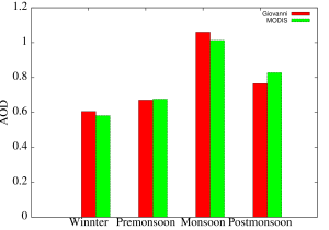
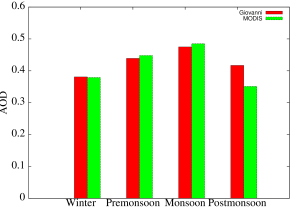
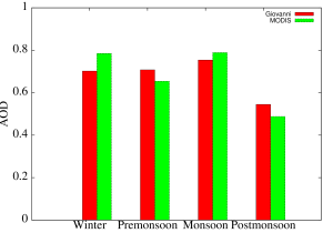
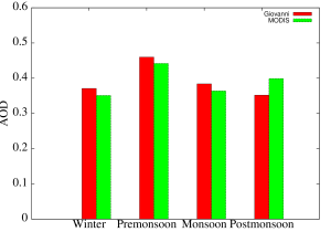
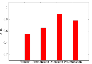
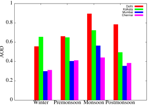
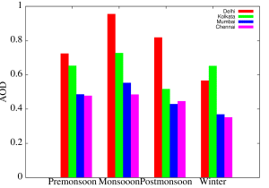
Figure 1 compares AOD data derived from MODIS level 2 and Giovanni level 3 for four megacities. MODIS data derived for 1 x 1 degree square area around the city center whereas Giovanni data are presented for nearest 1 x 1 degree grid. Figure 2(a) shows season-wise variation of AOD over Delhi. AOD data of last 13 years (2000-2012), averaged season wise, has been presented. This figure clearly shows seasonal variation. Figure 2(b) shows variation of averaged AOD for a particular season (premonsoon here) against different grid sizes for Delhi.

(a)

(b)

Figure 2: (a)Delhi AOD season wise (OD spatial resolution ) (b) Averaged AOD for a particular season (Premonsoon) from OD to QD over Delhi

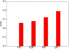
Averaged AOD increases monotonically as we approach city center from outskirts. Grid size for both these figure is 1 x 1 degree square. In figure 3 and 4 seasonal average value of AOD for four megacities have been presented in four spatial resolutions.

(a) Winter

(b) Premonsoon

(c) Monsoon

(d) Postmonsoon

Figure 3: Seasonal average value of AOD for four megacities in four spatial grids (error bars represent one standard deviation).

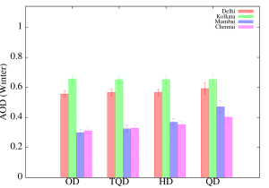
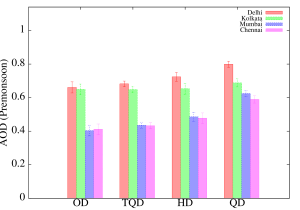
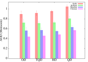
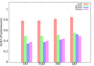
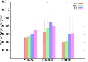
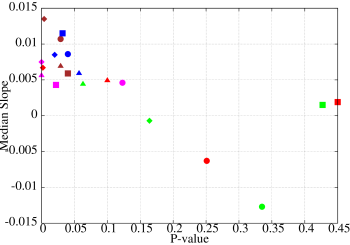
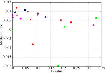
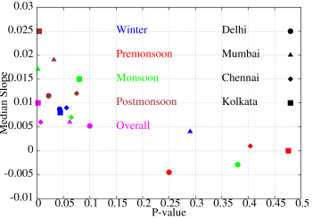
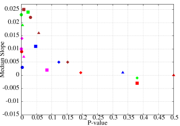
Delhi and Kolkata clearly registered higher values than Mumbai and Chennai. However for winter seasons Kolkata registered higher values even than Delhi. In figure 5 statistically significant (at p=0.05 level) overall median slopes of trend derived by Sen’s method is presented for 3 megacities. Since for Delhi there is no ’statistically significant’ trend (increasing/decreasing), slopes for Delhi have not been presented here. However from Table 2 it is evident that for seasons premonsoon and Winter Delhi showed prominent increasing trend. Different colours shows slopes at different grid sizes. Almost for all the cities median slopes of overall trends increases as we approach city centres. Table 2 clearly shows for OD and TQD grid sizes almost all the cities have increasing trend for AOD in case of winter and postmonsoon seasons. For Chennai we find there is an increasing trend of AOD for all the seasons in all grid sizes up to HD. Interestingly no city registered increasing trend for AOD in any spatial grids in the season of monsoon.

(a) OD

(b) HD

Figure 4: Comparison of seasonal average of AOD in four megacities

Table 2: Seasonal Median Slopes ( derived by Sen’s method ) of aerosol optical depth ( AOD) over four megacities ) for last 13 years (at p=0.05 level)

(OD)	Winter	Premonsoon	Monsoon	Postmonsoon	Overall
Delhi	$\uparrow$ 0.0087	No	No	$\uparrow$ 0.0015	NO
Mumbai	$\uparrow$ 0.006	$\uparrow$ 0.0047	No	$\uparrow$ 0.0063	$\uparrow$ 0.0052
Chennai	$\uparrow$ 0.0081	$\uparrow$ 0.0083	No	$\uparrow$ 0.0116	$\uparrow$ 0.0066
Kolkata	$\uparrow$ 0.0123	No	No	$\uparrow$ 0.0085	$\uparrow$ 0.004

TQD	Winter	Premonsoon	Monsoon	postmonsoon	Overall
Delhi	$\uparrow$ 0.0086	No	No	$\uparrow$ 0.0107	No
Mumbai	No	No	No	$\uparrow$ 0.0069	$\uparrow$ 0.0056
Chennai	$\uparrow$ 0.0085	$\uparrow$ 0.0067	No	$\uparrow$ 0.0135	$\uparrow$ 0.0075
Kolkata	$\uparrow$ 0.0115	No	No	$\uparrow$ 0.0059	$\uparrow$ 0.0043

(HD)	Winter	Premonsoon	Monsoon	Postmonsoon	Overall
Delhi	No	No	No	No	No
Mumbai	$\uparrow$ 0.008	$\uparrow$ 0.006	No	$\uparrow$ 0.008	$\uparrow$ 0.006
Chennai	$\uparrow$ 0.0083	$\uparrow$ 0.0108	No	$\uparrow$ 0.0149	$\uparrow$ 0.0082
Kolkata	No	No	No	No	$\uparrow$ 0.006

QD	Winter	Premonsoon	Monsoon	Postmonsoon	Overall
Delhi	$\uparrow$ 0.0096	No	No	No	No
Mumbai	No	No	——–	$\uparrow$ 0.0081	$\uparrow$ 0.007
Chennai	No	$\uparrow$ 0.0121	No	No	$\uparrow$ 0.0081
Kolkata	No	No	No	No	$\uparrow$ 0.0062
Chennai	No	$\uparrow$ 0.012	No	No	$\uparrow$ 0.008

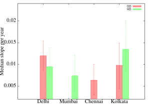
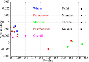
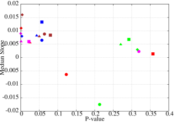
In figure 6 median slopes have been presented against p-values for all four seasons and for all four megacities including overall Kendall slope and in four grid sizes. In these figures different colours used to present different seasons whereas symbols represents different cities. For Ångström exponent we have considered two spatial resolutions OD and HD. Table 5 and figure 5 (b) shows median slopes of trend for varying spatial resolutions in case of Ångsröm exponent.

Table 3: Ångström exponent

OD	Winter	Premonsoon	Monsoon	Postmonsoon	Overall
Delhi	0.0265 $\uparrow$	0.0025 $\uparrow$	0.0122 $\uparrow$	0.0254 $\uparrow$	0.012 $\uparrow$
Mumbai	0.0185 $\uparrow$	No	-0.0156 $\downarrow$	0.0169 $\uparrow$	No
Chennai	No	No	No	No	0.0064 $\uparrow$
Kolkata	0.0253 $\uparrow$	0.0083 $\uparrow$	No	No	0.0098 $\uparrow$

HD	Winter	Premonsoon	Monsoon	Postmonsoon	Overall
Delhi	0.0216 $\uparrow$	0.0031 $\uparrow$	0.0088 $\uparrow$	0.0229 $\uparrow$	0.0095 $\uparrow$
Mumbai	No	No	No	0.0194 $\uparrow$	0.0074 $\uparrow$
Chennai	No	No	No	No	No
Kolkata	0.0251 $\uparrow$	0.0113 $\uparrow$	No	0.0241 $\uparrow$	0.0135 $\uparrow$

Table 4: Comparison of Median slopes (Overall) of aerosol optical depth ( AOD) for 13 years for four megacities in four spatial resolutions (at p=0.05 level)

	OD	TQD	HD	QD
Delhi	No	No	No	No
Mumbai	$\uparrow$ 0.0052	$\uparrow$ 0.0056	$\uparrow$ 0.006	$\uparrow$ 0.007
Chennai	$\uparrow$ 0.0066	$\uparrow$ 0.0075	$\uparrow$ 0.006	$\uparrow$ 0.00862
Kolkata	$\uparrow$ 0.004	$\uparrow$ 0.0043	$\uparrow$ 0.006	$\uparrow$ 0.0062

The study clearly shows AOD is increasing in three of the four Indian megacities even when seasonal effects are considered. Only Delhi registered no significant overall increase corroborating earlier studies but one should remember AOD over Delhi is already very high compared to other cities. However Delhi registered significant increasing trend in winter and postmonsoon seasons in some spatial grids[Table 2, fig. 6]. City centres not only are already high in AOD, rate of increase is also higher in city centres compared to outskirts. In case of Ångström exponent the scenario is more or less the same. Since higher Ångström exponent means lower particle size, increase in this exponent points to more hazards to public health because smaller particles are known to cause more severe problems[5, 4]. The case of Delhi should be considered here specially, Delhi has not registered any significant growth in AOD but it has shown significant increasing trend in case of Ångström exponent. Although ground based measurements are best to reach any concrete conclusion, satellite sensed data averaged by seasons and compared for long time undoubtedly gives an overview how and at which rate our cities are getting polluted as time goes and hopefully this study will come handy to policymakers and researcher for more detailed studies.

Table 5: Comparison of Median slopes (Overall) Ångström exponent for 13 years for four megacities in two spatial resolutions (at p=0.05 level)

	OD	HD
Delhi	0.012 $\uparrow$	0.0095 $\uparrow$
Mumbai	NO	0.0074 $\uparrow$
Chennai	0.0064 $\uparrow$	No
Kolkata	0.0098 $\uparrow$	0.0135 $\uparrow$

(a) AOD

(b) Ångström Exponent($\alpha$) (0.47 - 0.66 $\mu m$ )

Figure 5: Overall Median Slopes of trend for A. AOD and B. Ångström exponent($\alpha$) of megacities in various spatial resolutions (error bars represents lower and upper limits of 80 % confidence interval and have been calculated using formulae 7 and 8. )

(a) OD

(b) TQD

(c) HD

(d) QD

Figure 6: P-value vs Median slope of AOD trend for four megacities in four spatial resolution

(a) Grid size OD

(b) Grid size HD

Figure 7: Median slopes of trend vs p-value of Ångström exponent($\alpha$) for four megacities in two spatial resolution

Acknowledgements:

We thank the entire MODIS science team for providing us data used in this study.

References

- [1] Kaufman, Y. J., Gitelson, A., Karnieli, A., Ganor, E., Fraser, R. S., Nakajima, T., Matoo, S., and Holben, B. N.: Size distribution and scattering phase function of aerosol particles retrieved from sky brightness measurements, Geophys. Res. Let., 99, 10 341–10 356, 1994.
- [2] Ramachandran S., Kedia S., Srivastava R., Aerosol optical depth trends over different reguions of India, Atmospheric Environment, 49 (2012) 338-347
- [3] Molina, M. J. Molina and L. T. Molina, Megacities and atmospheric pollution, Journal of the air and waste management association, vol 54, no. 6, 2004,pp. 644-680.
- [4] C. Arden Pope III and Dockery D. W., (2006) Health Effects of Fine Particulate Air Pollution: Lines that Connect, Journal of the Air & Waste Management Association, 56:6, 709-742, DOI: 10.1080/10473289.2006.10464485
- [5] Pope C. A., Ezzati M. and Dockery D W , Fine Particulate Air Pollution and US County Life Expectancies, n final edited form as: N Engl J Med . 2009 January 22; 360(4): 376–386
- [6] Samoli E., et al, Estimating the exposure-response relationships between particulate matter and mortality within the APHEA multicity project. Environ Health Perspect. 2005 Jan;113(1):88-95.
- [7] Seinfeld J. H., Pandis, S.N., Atmospheric chemistry and physics: From air pollution to climate change. john Willey and Sons.
- [8] Remer L. A. et al, The MODIS Aerosol Algorithm, Products and Validation,Journal of the Atmospheric Science, 2005.
- [9] Olga S. and Pavel K, AOD Trends over megacities based on space monitoring using MODIS and MISR, American Journal of Climate Change, 2012,1,117-131.
- [10] Gupta P, Khan M N, Silva A, Patadia F, MODIS aerosol optical depth observation over urban areas in Pakistan: quantity and quality of the data for monitoring, Atmospheric pollution research 4 2013 43-52.
- [11] Acharya P and Sreekesh S., Seasonal variability in aerosol optical depth over India: a spatio-temoral analysis using the MODIS aerosol product, International Journal of remote sensing, Vol. 34, No. 13, 4832-4849.
- [12] T. Brinkhoff, “The principal agglomeration of the world”, 2010, http://www.citypopulation.de
- [13] Ångström, A. K.: On the atmospheric transmission of sun radiation and on the dust in the air, Geogr. ANN., 12, 130–159, 1929.
- [14] Remer et al, Algorithm for remote sensing of tropospheric aerosol form Modis: Collection 5.
- [15] Chattopadhyay G., Chakraborthy P. & Chattopadhyay S., Mann–Kendall trend analysis of tropospheric ozone and its modeling using ARIMA, Theor Appl Climatol (2012) 110:321–328
- [16] Gilbert R. (1987), Statistical Methods for Environmental Pollution Monitoring, Van Nostrand Reinhold Company inc.
- [17] Mann, H. B., Non-parametric tests against trend, Econometrica, 13, 245-259,1945.
- [18] Hirsch, R. M., J. R. Slack, and R. A. Smith, Techniques of trend analysis for monthly water quality data, Water Resources Research, 18(1), 107-121, 1982.
- [19] Sen, P. K., 1968b. Estimates of the regression coefficient based on Kendall’s tau, Journal of the American Statistical Association 63:1379-1389.
- [20] Remer et al, A critical look at deriving monthly aerosol optical depth from satellite data, IEEE Transactions on geoscience and remote sensing, Vol. 47, No. 8, 2009.