Does a strong particle accelerator arise very close to the light cylinder in a pulsar magnetosphere?

Abstract

We examine if an efficient particle acceleration takes place by a magnetic-field-aligned electric field near the light cylinder in a rotating neutron star magnetosphere. Constructing the electric current density with the actual motion of collision-less plasmas, we express the rotationally induced, Goldreich-Julian charge density as a function of position. It is demonstrated that the ‘light cylinder gap’, which emits very high energy photons via curvature process by virtue of a strong magnetic-field-aligned electric field very close to the light cylinder, will not arise in an actual pulsar magnetosphere.

1 Introduction

The Crab pulsar (PSR J0534+2200), one of the youngest pulsars in our Galaxy, shows pulsed signals in a very wide energy range from radio to $\gamma$-rays (e.g., see Abdo et al. 2010 for the observation of this pulsar with Fermi LAT between 100 MeV and 20 GeV). In the highest energy range, the Major Atmospheric Gamma-Ray Imaging Cherenkev (MAGIC) telescope has detected pulsed signals at 25 GeV (Aliu et al. 2008), which was confirmed by the LAT observations (Atwood et al. 2009). Further observations with the MAGIC telescope and the Very Energetic Radiation Imaging Telescope Array System (VERITAS) have shown that this component extends up to 400 GeV (Aleksić et al. 2012; Aliu et al. 2011).

To explain such pulsed fluxes in the very high energy (VHE) region (i.e., above 100 GeV), Bednarek (2012) proposed the ‘light cylinder (LC) gap’ model from the following reasons: The rotationally induced, Goldreich-Julian (GJ) charge density is given by (Goldreich-Julian 1969) $\rho_{\rm GJ}=-\left[\mbox{\boldmath$\Omega$}\cdot\mbox{\boldmath$B$}/(2\pi c)\right]\left[1-(\varpi/\varpi_{\rm LC})^{2}\right]^{-1},$ where $\Omega$ denotes the rotation vector of the neutron star, $\Omega=|\mbox{\boldmath$\Omega$}|$ its rotation frequency, $B$ the magnetic field at each point, $\varpi$ the distance from the rotation axis, $\varpi_{\rm LC}=c/\Omega$ the radius of the LC measured from the rotation axis, and $c$ the speed of light. If the real charge density, $\rho_{\rm r}$, coincides $\rho_{\rm GJ}$ at every position, the magnetic-field-aligned electric field, $E_{\parallel}$, vanishes in the entire region of the magnetosphere. If $\rho_{\rm r}$ deviates from $\rho_{\rm GJ}$ at some position, on the other hand, the acceleration electric field $E_{\parallel}$ will arise around that position. In this expression, $\rho_{\rm GJ}$ appears to diverge at the LC, $\varpi\rightarrow\varpi_{\rm LC}$; thus, it was argued if $\rho_{\rm r}$ inevitably deviates from $\rho_{\rm GJ}$ near the LC. By virtue of this diverging behavior of $\rho_{\rm GJ}$, an extremely strong $E_{\parallel}$, which is about $10^{3}$ stronger than what arises in the outer-magnetospheric particle accelerator (or the outer gap), was assumed to arise in the LC gap, and the resultant curvature emission was implied to reproduce the pulsed spectrum observed from the Crab pulsar up to 400 GeV.

In § 2, we demonstrate that the LC gap model is not feasible, examining the actual $\rho_{\rm GJ}$ distribution. Then in § 3, we briefly mention an appropriate way to compute $\rho_{\rm GJ}$.

2 Goldreich Julian charge density in the outer magnetosphere

In the special relativistic limit, the GJ charge density is given by (e.g., Mestel & Wang 1982)

$$\rho_{\rm GJ}\equiv-\frac{\mbox{\boldmath$\Omega$}\cdot\mbox{\boldmath$B$}}{2\pi c}+\frac{(\mbox{\boldmath$\Omega$}\times\mbox{\boldmath$r$})\cdot(\nabla\times\mbox{\boldmath$B$})}{4\pi c}.$$ (1)

From the inhomogeneous part of the Maxwell equations, we obtain,

$$\nabla\times\mbox{\boldmath$B$}=\frac{4\pi}{c}\mbox{\boldmath$J$}+\frac{1}{c}\frac{\partial\mbox{\boldmath$E$}}{\partial t}.$$ (2)

Since the plasmas are highly collision-less in a pulsar magnetosphere, charged particles gyrate many times between collisions. Thus, we must construct the electric current $J$ from the gyrating and drifting motion of charged particles, not from the generalized Ohm’s law. Let us decompose the current into the parallel and perpendicular components with respect to the local magnetic field line,

$$\mbox{\boldmath$J$}=\mbox{\boldmath$J$}_{\parallel}+\mbox{\boldmath$J$}_{\perp}.$$ (3)

First, we consider the parallel current. Since the radiation force balances with the electrostatic acceleration, particles’ distribution becomes mono-energetic. Thus, denoting the terminal velocity of out-going particles (e.g., positrons) with $\mbox{\boldmath$v$}_{\parallel+}$, and in-going ones (e.g., electrons) with $\mbox{\boldmath$v$}_{\parallel-}$, we obtain

$$\mbox{\boldmath$J$}_{\parallel}=e(n_{+}\mbox{\boldmath$v$}_{\parallel+}-n_{-}\mbox{\boldmath$v$}_{\parallel-})$$ (4)

where $n_{+}$ (or $n_{-}$) denotes the number density of out-going (or in-going) particles, and $\mbox{\boldmath$v$}_{\parallel\pm}$ is given by (Hirotani 2011, ApJ 733, L49)

$$\mbox{\boldmath$v$}_{\parallel\pm} = cf_{\pm}\frac{\mbox{\boldmath$B$}}{B},$$

$$f_{\pm} \equiv -\frac{\varpi}{\varpi_{\rm LC}}\frac{B^{\hat{\varphi}}}{B}\pm\sqrt{1-\left(\frac{\varpi}{\varpi_{\rm LC}}\right)^{2}\left(\frac{B_{\rm p}}{B}\right)^{2}};$$ (5)

$e$ denotes the charge on the out-going particle (presumably the positron), $B_{\rm p}^{2}=B^{2}-(B^{\hat{\varphi}}{})^{2}$, and $B^{\hat{\varphi}}$ the toroidal component of the magnetic field. In the higher altitudes (e.g., near the LC), it is reasonable to assume $n_{+}\gg n_{-}$ in the gap. In this case, the real charge density is given by $\rho_{\rm r}=e(n_{+}-n_{-})\approx en_{+}$. Thus, we obtain

$$\mbox{\boldmath$J$}_{\parallel}=\rho_{\rm r}\mbox{\boldmath$v$}_{\parallel+}$$ (6)

Even if $n_{-}\approx n_{+}$, the additional term that would appear in the right-hand side will not change the entire discussion of this paper; however, we assume $n_{-}\ll n_{+}$ to clarify the logic.

Second, we consider the perpendicular current. It is given by

$$\mbox{\boldmath$J$}_{\perp} = c\rho_{\rm r}\frac{\mbox{\boldmath$E$}\times\mbox{\boldmath$B$}}{B^{2}}+c(P_{\perp}+P_{\parallel})\frac{\mbox{\boldmath$B$}}{B^{2}}\times\frac{\nabla B}{B}$$ (7)

$$+\frac{c^{2}\rho}{B^{2}}\dot{\mbox{\boldmath$E$}}_{\perp}-c\nabla\times\left(P_{\perp}\frac{\mbox{\boldmath$B$}}{B^{2}}\right),$$

where $P_{\parallel}$ and $P_{\perp}$ denote the pressure associated with the longitudinal and perpendicular motion with respect to the magnetic field; $\rho$ (in the second line) denotes the mass density of the plasmas, and $\dot{\mbox{\boldmath$E$}}_{\perp}$ the temporal derivative of the electric field projected on the perpendicular plane to $B$. In the right-hand side, the first term represents the current due to the $E\times B$ drift, the second term the sum of the currents due to the magnetic-gradient and the magnetic-curvature drift, the third term (in the second line) the polarization-drift current, and the last term the magnetization current. In a collision-less plasma, the pressure tensor becomes highly anisotropic. In a pulsar magnetosphere, pairs are created inwards (via photon-photon and/or magnetic pair creation in the middle or lower altitudes) with the typical Lorentz factor of a few thousand. Thus, positrons (or electrons) lose most of their perpendicular momentum when they return outwards by a positive (or a negative) $E_{\parallel}$ in a strong magnetic field. Moreover, their pitch angles decrease due to a subsequent acceleration by $E_{\parallel}$, resulting in $P_{\perp}\ll P_{\parallel}$. Thus, for particles migrating in the outer magnetosphere, we obtain

$$\mbox{\boldmath$J$}_{\perp}=c\rho_{\rm r}\frac{\mbox{\boldmath$E$}\times\mbox{\boldmath$B$}}{B^{2}}+cP_{\parallel}\frac{\mbox{\boldmath$B$}}{B^{2}}\times\frac{\nabla B}{B}+\frac{c^{2}\rho}{B^{2}}\dot{\mbox{\boldmath$E$}}_{\perp}.$$ (8)

In a co-rotating magnetosphere, we can put $\rho_{\rm r}=\rho_{\rm GJ}$ and have $c\mbox{\boldmath$E$}\times\mbox{\boldmath$B$}=(\mbox{\boldmath$\Omega$}\times\mbox{\boldmath$r$})B^{2}$. Thus, combining equations (1), (2), (3), (6), and (8), we obtain

$$\left[1-\left(f_{+}\frac{B^{\hat{\phi}}}{B}+\frac{\gamma m_{\rm e}c^{2}}{eB}\frac{b^{\hat{\varphi}}}{L}+\frac{m_{\rm e}c\dot{E}^{\hat{\varphi}}}{eB^{2}}\right)\frac{\varpi}{\varpi_{\rm LC}}-\left(\frac{\varpi}{\varpi_{\rm LC}}\right)^{2}\right]\rho_{\rm GJ}$$ (9)

$$= -\frac{\mbox{\boldmath$\Omega$}\cdot\mbox{\boldmath$B$}}{2\pi c}+\frac{\mbox{\boldmath$e$}_{\hat{\varphi}}\cdot\dot{E}}{4\pi c}\frac{\varpi}{\varpi_{\rm LC}},$$

where

$$\frac{b^{\hat{\varphi}}}{L}\equiv\mbox{\boldmath$e$}_{\hat{\varphi}}\cdot\left(\frac{\mbox{\boldmath$B$}}{B}\times\frac{\nabla B}{B}\right),$$ (10)

$L\sim\varpi_{\rm LC}$, $|b^{\hat{\varphi}}|\sim 1$, and $\mbox{\boldmath$e$}_{\hat{\varphi}}$ denotes the toroidal unit vector. Note that $\gamma m_{\rm e}c^{2}$ is much small compared to $eBL$ if particles efficiently radiate, and that $|\dot{E}^{\hat{\varphi}}|<\Omega B$. We thus finally obtain

$$\rho_{\rm GJ}=\frac{\displaystyle{-\frac{\mbox{\boldmath$\Omega$}\cdot\mbox{\boldmath$B$}}{2\pi c}+\frac{\mbox{\boldmath$e$}_{\hat{\varphi}}\cdot\dot{E}}{4\pi c}\frac{\varpi}{\varpi_{\rm LC}}}}{\displaystyle{1-f_{+}\frac{B^{\hat{\phi}}}{B}\frac{\varpi}{\varpi_{\rm LC}}-\left(\frac{\varpi}{\varpi_{\rm LC}}\right)^{2}}}$$ (11)

In the numerator, the second term is usually small compared to the first term. In the denominator, we should notice that $f_{+}$ is positive definite, provided $B^{\hat{\phi}}<0$. For example, at the LC, we obtain $f_{+}=2|B^{\hat{\varphi}}|/B$. Thus, we find

$$-f_{+}\frac{B^{\hat{\phi}}}{B}\frac{\varpi}{\varpi_{\rm LC}}>0.$$ (12)

It follows that the denominator of equation (11) does not vanish at the LC, provided that the magnetic field is toroidally bent. Moreover, near the LC, we obtain

$$-f_{+}\frac{B^{\hat{\phi}}}{B}\frac{\varpi}{\varpi_{\rm LC}}\approx 1.$$ (13)

Therefore, the GJ charge density is kept around its Newtonian value, $-\mbox{\boldmath$\Omega$}\cdot\mbox{\boldmath$B$}/(2\pi c)$, even near the LC.

We can confirm this result by substituting the solution of the vacuum, rotating dipole magnetic field (Cheng et al. 2000) into equation (1). In figure 1, we plot $\rho_{\rm GJ}/[\Omega B/(2\pi c)]$ as a function of the distance along each magnetic field line. The magnetic inclination angle $\alpha$ between the magnetic and rotational axes, is assumed to be $60^{\circ}$ for the solid, dashed, dotted curves, whereas $0^{\circ}$ for the dot-dot-dot-dashed one. The solid (or dashed) curves show the results in the trailing (or leading) side of the rotating magnetosphere. The filled circle denotes the position at which the field line crosses the light cylinder. It is confirmed by this explicit calculation that $\rho_{\rm GJ}$ is kept around its Newtonian value even near the LC.

The conclusion is unchanged for small inclination angles. Adopting the vacuum rotating magnetic dipole solution, we obtain $B^{\hat{\phi}}=0$ if $\alpha=0^{\circ}$. As a result, equation (11) appears to give a diverging $\rho_{\rm GJ}$ at the LC. Nevertheless, the vacuum solution gives $\nabla\times\mbox{\boldmath$B$}=0$ when $\alpha=0^{\circ}$. Thus, equation (1) shows that $\rho_{\rm GJ}$ exhibits no singular behavior at the LC. We plot the case of $\alpha=0^{\circ}$ as the dot-dot-dot-dashed curve in figure 1, calculating equation (1) from the vacuum, rotating dipole solution. It follows that $\rho_{\rm GJ}$ does not change rapidly at the LC also for an aligned rotator, as expected.

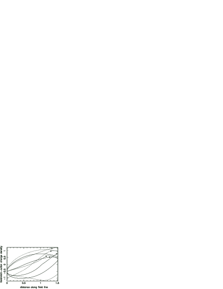
Figure 1: Distribution of the dimensionless Goldreich-Julian charge density, $\rho_{\rm GJ}/(\Omega B/2\pi c)$, as a function of the distance along the last-open magnetic field line, for discrete values of azimuthal angles, $\varphi_{\ast}$, measured counter-clockwise around the magnetic axis on the polar-cap surface. Magnetic inclination angle is assumed to be $60^{\circ}$ for the solid, dashed, and dotted curves, while $0^{\circ}$ for the dot-dot-dot-dashed one. The solid curves represent $\rho_{\rm GJ}/(\Omega B/2\pi c)$ in the trailing side of the rotating magnetosphere (from the top, $\varphi_{\ast}=-45^{\circ}$, $\varphi_{\ast}=-90^{\circ}$, $\varphi_{\ast}=-135^{\circ}$, and $\varphi_{\ast}=-180^{\circ}$) , while the dashed ones in the leading side (from the top, $\varphi_{\ast}=-45^{\circ}$, $\varphi_{\ast}=-90^{\circ}$, and $\varphi_{\ast}=-135^{\circ}$) . The rotational and magnetic axes, as well as the footpoints of the magnetic field lines of $\varphi_{\ast}=180^{\circ}$ and $\varphi_{\ast}=0^{\circ}$ at the polar-cap surface, reside on the same meridional plane. From the magnetic pole, the direction $\varphi_{\ast}=180^{\circ}$ points the rotation axis, while $\varphi_{\ast}=0^{\circ}$ the equator. The filled circle denotes the position at which the distance from the rotation axis becomes the light cylinder radius.

Recently, Bednarek (2012) assumed that $\rho_{\rm GJ}$ becomes as large as $\sim 10^{3}\Omega B/(2\pi c)$ in a short length $\sim 10^{-3}\varpi_{\rm LC}$ along the magnetic field line in the vicinity of the LC, and considered the curvature radiation that reproduces the pulsed emissions up to 400 GeV from the Crab pulsar. However, since $\rho_{\rm GJ}$ is kept of the order of $\Omega B/(2\pi c)$ even at the LC, this assumption cannot be justified. In another word, the light cylinder gap, which is suggested to produce the pulsed VHE emission from the Crab pulsar, does not appear in any pulsar magnetosphere.

3 Discussion

We arrive at the conclusion that the Goldreich-Julian charge density does not show any singular behavior at the light cylinder. We may note, in passing, that the Goldreich-Julian charge density should be computed from equation (1) directly, using the given magnetic field distribution in the three-dimensional rotating magnetosphere, instead of replacing $\nabla\times\mbox{\boldmath$B$}$ with the current (i.e., instead of using eq. [11]). We should notice here that we derive equation (1) only from the Maxwell equation, $\nabla\cdot\mbox{\boldmath$E$}=4\pi\rho_{\rm r}$, and the frozen-in condition, assuming stationarity in the co-moving frame, namely $F_{\mu t}+\Omega F_{\mu\varphi}=-\partial_{\mu}\Psi(r,\theta,\varphi-\Omega t)$, where $F_{\mu\nu}$ represents the field-strength tensor, $\Psi$ the non-corotational potential, and $\mu=t,r,\theta,\varphi$ (Hirotani 2006). That is, equation (1) holds for arbitrary magnetic field, and is derived irrespective of how the current is constructed, or how the plasmas are collisional or collision-less.

Let us briefly perform a thought experiment. If the plasma density is large enough, sufficient collisions allow us to use the generalized Ohm’s law to describe the current. In this case, $\rho_{\rm GJ}$ does not diverge at the LC, because the $-(\varpi/\varpi_{\rm LC})^{2}$ term in the coefficient of $\rho_{\rm GJ}$ in equation (9) comes from the $\mbox{\boldmath$E$}\times\mbox{\boldmath$B$}$ drift, which is not included in the Ohm’s law. For example, the magnetohydrodynamic approximation, which uses the Ohm’s law to close the equations, shows that all the physical quantities are well-behaved at the LC (e.g., Tchekhovskoy et al. 2013). Next, imagine that the plasmas suddenly escape from the magnetosphere to become collision-less. Even in this case, $\rho_{\rm GJ}$ should not be changed at all, because $\rho_{\rm GJ}$ is determined only by the $B$ field through equation (1), independently from the collisional status of plasmas. Thus, $\rho_{\rm GJ}$ does not diverge at the LC also in the collision-less limit. For example, in the force-free limit, which adopts the $\mbox{\boldmath$E$}\times\mbox{\boldmath$B$}$ drift in $\mbox{\boldmath$J$}_{\perp}$, no physical quantities diverge or rapidly change at the LC (e.g., Spitkovsky 2006), except for the current sheet, in which the force-free approximation breaks down.

In general, quantities behave normally across the LC, without showing any divergence or quick variations. Thus, the light cylinder gap, which has an extreme acceleration electric field (as $10^{3}$ times stronger than the outer gap), will not arise in a pulsar magnetosphere, unfortunately.

References

- 2012 ((2012)) Aleksić, J. et al. 2012, AA 540, 69
- Aliu (2011) Aliu, E. Arlen, T., Aune, T., et al. 2011, Science 334, 69
- Atwood et al. (2009) Atwood, W. B. et al. 2009, ApJ 697, 1071
- Bednarek (2013) Bednarek, W. 2013, MNRAS, 424, 2079
- Cheng et al. (2000) Cheng, K. S., Ruderman, M. & Zhang, L. 2000, ApJ 537, 964
- Goldreich, & Julian (1969) Goldreich, P. & Julian, W. H. 1969, ApJ 157, 869
- Hirotani (2006) Hirotani, K. 2006, MPLA21, 1319
- Hirotani (2011) Hirotani, K. 2011, ApJ, 733, L49
- Mestel & Wang (1982) Mestel, L., & Wang, Y. -M. 1982, MNRAS, 198, 405
- Spitkovsky (2006) Spitkovsky, A. 2006, ApJ 648, L51
- Tchekkovskoy et al. (2013) Tchekhovskoy, A., Spitkovsky, A., Li, J. G. 2013, MNRAS 435, L1