Transient acceleration in $f(T)$ gravity^∗

Abstract

Recently a $f(T)$ gravity based on the modification of the teleparallel gravity was proposed to explain the accelerated expansion of the universe without the need of dark energy. We use observational data from Type Ia Supernovae, Baryon Acoustic Oscillations, and Cosmic Microwave Background to constrain this $f(T)$ theory and reconstruct the effective equation of state and the deceleration parameter. We obtain the best-fit values of parameters and find an interesting result that the constrained $f(T)$ theory allows for the accelerated Hubble expansion to be a transient effect.

1 Introduction

A series of independent cosmological observations including the type Ia supernovae (SNIa) (Riess et al. 1998), large scale structure (Tegmark et al. 2004), baryon acoustic oscillation (BAO) peaks (Eisenstein et al. 2005) and cosmic microwave background (CMB) anisotropy (Spergel et al. 2003) have probed the accelerating expansion of the universe. Subsequently, many gravitational theories and cosmological models have been proposed to explain this cosmological phenomenon. Under the assumption of cosmological principles, these theories include the mysterious dark energy with negative pressure in general relativity and modify gravity models to the general relativity. For the former, the acceleration is realized by the drive of exotic dark energy, such as the cosmological constant, quintessence or phantom. The cosmological constant model ($\Lambda$CDM) is the simplest candidate for dark energy models, and agrees well with current cosmological observations. However, the $\Lambda$CDM model is faced with the fine-tuning problem (Weinberg 1989) and coincidence problem (Zlatev et al. 1999). Moreover, the nature of dark energy in form of other candidates still cannot be revealed. For the latter, the acceleration is realized by modification to the general relativity without exotic dark energy, such as the brane-world Dvali-Gabadadze-Porrati model (Dvali et al. 2000), $f(R)$ gravity (Chiba 2003), Gauss-Bonnet gravity (Nojiri & Odintsov 2005).

Similar as the exotic dark energy and other modified gravity models, it is found that the cosmic acceleration can also be obtained successfully from another gravitational scenario described by the $f(T)$ theory (Bengochea & Ferraro 2009). Proposed based on the Teleparallel Equivalent of General Relativity (also known as Teleparallel Gravity), scalar $T$ is the Lagrangian of teleparallel gravity. The teleparallel gravity is not a new theory of gravity, but an alternative geometric formulation of the general relativity. In teleparallel gravity, the Levi-Civita connection used in Einstein’s general relativity is replaced by the Weitzenböck connection with torsion. However, the torsion vanishes in the dark energy and modified gravity models. Moreover, $f(T)$ theories have several interesting features: they not only can explain the late accelerating expansion, but also have second order differential equations, which are simpler than the $f(R)$ gravity. In addition, when certain conditions are satisfied, the behavior of $f(T)$ will be similar to quintessence (Xu et al. 2012). Although $f(T)$ gravity has attracted wide attention, a disadvantage pointed out in Ref. (Li et al. 2011a) is that the action and the field equations of $f(T)$ do not respect local Lorentz symmetry. Nonetheless, the $f(T)$ gravity might provide a significant alternative to conventional dark energy in general relativistic cosmology. In addition, the Ref. (Saveliev et al. 2011) indicated that the Lorentz invariance violation is still possible, while $f(T)$ gravity might provide some insights about Lorentz violation. Such $f(T)$ theories are worth further depth studies.

Up to now, a number of $f(T)$ theories have been proposed (Bengochea & Ferraro 2009; Linder 2010; Yang 2011b; Myrzakulov 2011; Bamba et al. 2011; Wu & Yu 2011). Under these cases, Yang found that $f(T)$ theories are not dynamically equivalent to teleparallel action with an added scalar field (Yang 2011a). Like other gravity theories and models, the $f(T)$ theories also have been investigated using the popular observational data. Investigations show that the $f(T)$ theories are compatible with observations (see e.g. (Nesseris et al. 2013; Zheng & Huang 2011b) and references therein). We note that the new type of $f(T)$ theory was proposed to explain the accelerating expansion of the universe, and it behaves like a cosmological constant; but because of its dynamic behavior, it is free from the coincidence problem seen in the case of $\Lambda$CDM (Yang 2011b). Due to this characteristic, this type of $f(T)$ is possible to be distinguished from a $\Lambda$CDM model. However, observational analysis for this model is still absent. Hence, we would like to perform some further analysis using the observational data, such as the SNIa, BAO, and CMB.

This paper is organized as follows. In Sec 2, the general $f(T)$ gravity and the $f(T)$ model proposed in (Yang 2011b) are introduced. In Sec 3, we describe the method for constraining cosmological models and reconstruction scheme. Subsequently, the parameters of the specific $f(T)$ model are constrained by observational data. Further more, through the reconstruction scheme the effective equation of state and the deceleration parameter are reconstructed in Sec 4. Finally, we give the summary and conclusions in Sec 5.

2 The $f(T)$ theory

The $f(T)$ theory is a modification of teleparallel gravity, which uses the curvatureless Weitzenböck connection instead of torsionless Levi-Civita connection in Einstein’s General Relativity. The curvatureless torsion tensor is

$$T^{\lambda}_{\>\>\mu\nu}\equiv e^{\lambda}_{i}(\partial_{\mu}e^{i}_{\nu}-\partial_{\nu}e^{i}_{\mu}),$$ (1)

where $e^{\mu}_{i}$ $(\mu=0,1,2,3)$ are components of the four linearly independent vierbein field ${\mathbf{e}_{i}(x^{\mu})}$ ($i=0,1,2,3$) in a coordinate basis. In particular, the vierbein is an orthonormal basis for the tangent space at each point $x^{\mu}$ of the manifold: $\mathbf{e}_{i}\cdot\mathbf{e}_{j}=\eta_{i\,j}$, where $\eta_{i\,j}=$diag $(1,-1,-1,-1)$. Notice that Latin indices refer to the tangent space, while Greek indices label coordinates on the manifold. The metric tensor is obtained from the dual vierbein as $g_{\mu\nu}(x)=\eta_{i\,j}\,e^{i}_{\mu}(x)\,e^{j}_{\nu}(x)$. The torsion scalar is the Lagrangian of teleparallel gravity (Bengochea & Ferraro 2009)

$$T\equiv S_{\rho}^{\>\>\>\mu\nu}\>T^{\rho}_{\>\>\>\mu\nu},$$ (2)

where

$$S_{\rho}^{\>\>\>\mu\nu}=\frac{1}{2}\Big{(}K^{\mu\nu}_{\>\>\>\>\rho}+\delta^{\mu}_{\rho}\>T^{\theta\nu}_{\>\>\>\>\theta}-\delta^{\nu}_{\rho}\>T^{\theta\mu}_{\>\>\>\>\theta}\Big{)},$$ (3)

and the contorsion tensor $K^{\mu\nu}_{\>\>\>\>\rho}$ is given by

$$K^{\mu\nu}_{\>\>\>\>\rho}=-\frac{1}{2}\Big{(}T^{\mu\nu}_{\>\>\>\>\rho}-T^{\nu\mu}_{\>\>\>\>\rho}-T_{\rho}^{\>\>\>\>\mu\nu}\Big{)}.$$ (4)

In the $f(T)$ theory, we allow the Lagrangian density to be a function of $T$ (Bengochea & Ferraro 2009; Ferraro & Fiorini 2007; Linder 2010), thus the action reads

$$I=\frac{1}{16\,\pi\,G}\,\int d^{4}x\>e\>f(T),$$ (5)

where $e=det(e^{i}_{\mu})=\sqrt{-g}$. The corresponding field equation is

$$[e^{-1}\partial_{\mu}(e\>S_{i}^{\>\>\>\mu\nu})-e_{i}^{\>\lambda}\>T^{\rho}_{\>\>\>\mu\lambda}\>S_{\rho}^{\>\>\>\nu\mu}]f_{T}+S_{i}^{\>\>\>\mu\nu}\partial_{\mu}Tf_{TT}+\frac{1}{4}\>e_{i}^{\nu}\>f(T)=\frac{1}{2}k^{2}\>e_{i}^{\>\>\>\rho}\>T_{\rho}^{\>\>\>\nu},$$ (6)

where $k^{2}=8\pi G$, $f_{T}\equiv df/dT$, $f_{TT}\equiv d^{2}f/dT^{2}$, $S_{i}^{\>\>\mu\nu}\equiv e_{i}^{\>\>\rho}S_{\rho}^{\>\>\mu\nu}$, and $T_{\mu\nu}$ is the matter energy-momentum tensor. Obviously, Eq.(6) is a second-order equation. Thus, the $f(T)$ theories are simpler than the $f(R)$ theories with fourth-order equations.

Considering a flat homogeneous and isotropic FRW universe, we have

$$e^{i}_{\mu}={\rm diag}\left(1,a(t),a(t),a(t)\right)~{},~{}~{}~{}~{}e^{\mu}_{i}={\rm diag}\left(1,\frac{1}{a(t)},\frac{1}{a(t)},\frac{1}{a(t)}\right),$$ (7)

where $a(t)$ is the cosmological scale factor. By substituting Eqs.(7), (1), (3) and (4) into Eq. (2), we obtain the torsion scalar (Bengochea & Ferraro 2009)

$$T\equiv S^{\rho\mu\nu}T_{\rho\mu\nu}=-6\>H^{2},$$ (8)

where $H$ is the Hubble parameter $H=\dot{a}/a$. The dot represents the first derivative with respect to the cosmic time. Substituting Eq. (7) into (6), one can obtain the corresponding Friedmann equations

$$12H^{2}f_{T}+f=2k^{2}\rho,$$ (9)

$$48H^{2}\dot{H}f_{TT}-(12H^{2}+4\dot{H})f_{T}-f=2k^{2}p,$$ (10)

with $\rho$ and $p$ as the total energy density and pressure, respectively. The detailed calculation can be found in Ref. (Bengochea & Ferraro 2009). The conservation equation reads

$$\dot{\rho}+3H(\rho+p) = 0.$$ (11)

We should note that the only components considered here are matter and radiation, but not dark energy. After brief simplification to the Friedmann Eqs.(9) and (10), we can rewrite them as

$$\frac{3}{k^{2}}H^{2} = \rho+\rho_{\rm eff},$$ (12)

$$\frac{1}{k^{2}}(2\dot{H}+3H^{2}) = -(p+p_{\rm eff}),$$ (13)

where the effective energy density $\rho_{\rm eff}$ and pressure $p_{\rm eff}$ contributed from torsion are respectively given by (Yang 2011b)

$$\rho_{\rm eff} = \frac{1}{2k^{2}}(-12H^{2}f_{T}-f+6H^{2}),$$ (14)

$$p_{\rm eff} = -\frac{1}{2k^{2}}[48\dot{H}H^{2}f_{TT}-4\dot{H}f_{T}+4\dot{H}]-\rho_{\rm eff}.$$ (15)

We term it “effective” because it is just a geometric effect instead of a specific cosmic component. Therefore, what we are interested in is the acceleration driven by the torsion, not the exotic dark energy. Using Eqs.(14) and (15), we can define the total and effective equation of state as (Yang 2011b)

$$w_{\rm tot} \equiv \frac{p+p_{\rm eff}}{\rho+\rho_{\rm eff}}=-1+\frac{2(1+z)}{3H}\frac{dH}{dz},$$ (16)

$$w_{\rm eff} \equiv \frac{p_{\rm eff}}{\rho_{\rm eff}}=-1-\frac{48\dot{H}H^{2}f_{TT}-4\dot{H}f_{T}+4\dot{H}}{-12H^{2}f_{T}-f+6H^{2}}.$$ (17)

The deceleration parameter, as usual, is defined as

$$q(z)\equiv-\frac{\ddot{a}}{aH^{2}}=-1+\frac{(1+z)}{H}\frac{dH}{dz}.$$ (18)

After reviewing the general formation of $f(T)$ gravity, we now focus on a type of $f(T)$ gravity proposed in Ref. (Yang 2011b)

$$f(T)=T-\alpha T_{0}\big{[}\big{(}1+\frac{T^{2}}{T^{2}_{0}}\big{)}^{-n}-1\big{]},$$ (19)

which is analogue with a type of $f(R)$ theory proposed in Ref. (Starobinsky 2007), where $\alpha$ and $n$ are positive constants. $T_{0}=-6H^{2}_{0}$ and $H_{0}$ is the current value of the Hubble parameter. This type of $f(T)$ gravity has attracted much attention and been discussed in detail in Ref. (Sharif & Azeem 2012). Here we will look into the observational constraints on this type of $f(T)$ gravity. With $f(T)$ taking the form of Eq. (19), Eq.(9) can be rewritten as

$$E^{2}+\frac{4n\alpha E^{4}}{(1+E^{4})^{n+1}}+\frac{\alpha}{(1+E^{4})^{n}}-B=\alpha,$$ (20)

where $E^{2}\equiv H^{2}/H^{2}_{0}$ and $B=\Omega_{m0}(1+z)^{3}$, with $\Omega_{m0}$ being the matter density parameter today. Here we only focus on the evolution of the universe at low redshift, so we neglect the contribution of radiation. For $E(z=0)=1$, we have $\alpha=(1-\Omega_{m0})/(1-2^{-n+1}n-2^{-n})$. This $f(T)$ model has some interesting characteristics: firstly, the cosmological constant is zero in the flat space-time because $f(T=0)=0$, while the geometrical one attributes as the dark energy; secondly, it can behave like the cosmological constant. Such characteristics indicate that this type of $f(T)$ model is possible to be accepted by observational data, while impossible to be distinguished from the $\Lambda$CDM. Moreover, though the behavior of this type of $f(T)$ theory is similar to $\Lambda$CDM because of its dynamic behavior, it can avoid the coincidence problem suffered by $\Lambda$CDM.

3 Observational data and fitting method

In this section, we would like to introduce the observational data and constraint method. The corresponding observational data here are distance moduli of SNIa, CMB shift parameter and BAO distance parameter.

3.1 Type Ia supernovae

As early as 1998, cosmic accelerating expansion was first observed by ”standard candle” SNIa which has the same intrinsic luminosity. Therefore, the observable is usually presented in the distance modulus, the difference between the apparent magnitude $m$ and the absolute magnitude $M$. The latest version is Union2.1 compilation which includes 580 samples (Suzuki et al. 2012). They are discovered by the Hubble Space Telescope Cluster Supernova Survey over the redshift interval $0.01<z<1.42$. The theoretical distance modulus is given by

$$\mu_{th}(z)=m-M=5\log_{10}D_{L}(z)+\mu_{0},$$ (21)

where $\mu_{0}=42.38-5\log_{10}h$, and $h$ is the Hubble constant $H_{0}$ in the units of 100 km s^-1Mpc^-1. The corresponding luminosity distance function $D_{L}(z)$ is

$$D_{L}(z)=(1+z)\int_{0}^{z}\frac{dz^{\prime}}{E(z^{\prime};\textbf{p})},$$ (22)

where $E(z^{\prime};\textbf{p})$ is the dimensionless Hubble parameter given by Eq.(20), and p stands for the parameter vector of the evaluated model embedded in the expansion rate parameter $E(z)$. We note that parameters in the expansion rate $E(z)$ include the annoying parameter $h$. In order to exclude the Hubble constant, we should marginalize over the nuisance parameter $\mu_{0}$ by integrating the probabilities on $\mu_{0}$ (Pietro & Claeskens 2003; Nesseris & Perivolaropoulos 2005; Perivolaropoulos 2005). Finally, we can estimate the remaining parameters by minimizing

$$\tilde{\chi}^{2}_{\rm SN}(z,\textbf{p})=A-\frac{B^{2}}{C},$$ (23)

where

$$A(\textbf{p}) = \sum_{i}\frac{[\mu_{obs}(z)-\mu_{th}(z;\mu_{0}=0,\textbf{p})]^{2}}{\sigma_{i}^{2}(z)},$$

$$B(\textbf{p}) = \sum_{i}\frac{\mu_{obs}(z)-\mu_{th}(z;\mu_{0}=0,\textbf{p})}{\sigma_{i}^{2}(z)},$$

$$C = \sum_{i}\frac{1}{\sigma_{i}^{2}(z)},$$

and $\mu_{obs}$ is the observational distance modulus. This approach has been used in the reconstruction of dark energy (Wei et al. 2007), parameter constraint (Wei 2010), reconstruction of the energy condition history (Wu et al. 2012) etc.

3.2 Cosmic microwave background

The CMB experiment measures the temperature and polarization anisotropy of the cosmic radiation in early epoch. It generally plays a major role in establishing and sharpening the cosmological models. In the CMB measurement, the shift parameter $R$ is a convenient way to quickly evaluate the likelihood of the cosmological models, and contains the main information of the CMB observation (Hu & Sugiyama 1996; Hinshaw et al. 2009). It is expressed as

$$R=\sqrt{\Omega_{m0}}\int^{z_{s}}_{0}\frac{dz^{\prime}}{E(z^{\prime};\textbf{p})},$$ (24)

where $z_{s}=1090.97$ is the redshift of decoupling. According to the measurement of WMAP-9 (Hinshaw et al. 2013), we estimate the parameters by minimizing the corresponding $\chi^{2}$ statistics

$$\chi^{2}_{R}=\left(\frac{R-1.728}{0.016}\right)^{2}.$$ (25)

3.3 Baryon acoustic oscillation

The measurement of BAO in the large-scale galaxies has rapidly become one of the most important observational pillars in cosmological constraints. This measurement is usually called the standard ruler in cosmology (Eisenstein & Hu 1998). The distance parameter $A$ obtained from the BAO peak in the distribution of SDSS luminous red galaxies (Eisenstein et al. 2005) is a significant parameter and defined as

$$A_{th}=\Omega_{m0}^{1/2}E(z_{1})^{-1/3}\left[\frac{1}{z_{1}}\int^{z_{1}}_{0}\frac{dz^{\prime}}{E(z^{\prime};\textbf{p})}\right]^{2/3}.$$ (26)

We use the three combined data points in Ref. (Addison et al. 2013) that cover $0.1<z<2.4$ to determine the parameters in evaluated models. The expression of $\chi^{2}$ statistics is

$$\chi^{2}_{\rm{A}}=\sum_{i}\left(\frac{A_{th}-A_{obs}}{\sigma^{2}_{A}}\right)^{2},$$ (27)

where $A_{obs}$ is the observational distance parameter and $\sigma_{A}$ is its corresponding error.

Since the SNIa, CMB, and BAO data points are effectively independent measurements, we can simply minimize their total $\chi^{2}$ values

$$\chi^{2}(z,\textbf{p})=\tilde{\chi}^{2}_{\rm SN}+\chi^{2}_{\rm R}+\chi^{2}_{\rm A},$$

to determine the parameters in the evaluated $f(T)$ model.

3.4 Reconstructing method

Using the above introduced $\chi^{2}$ statistics, we can obtain the best-fit values and their errors of basic parameters p. Further, we can reconstruct the other variable $F$ relative with the known basic parameters p by error propagation following the method in Ref. (Lazkoz et al. 2012). For example, the estimation from the observational data on the $i$th parameter $p_{i}$ is $p_{i}={p_{0i}}^{+\sigma_{iu}}_{-\sigma_{il}}$, where $p_{0i}$ is the best-fit value, $\sigma_{iu}$ and $\sigma_{il}$ are the upper limit and lower limit, respectively. Errors of the reconstructed function $F$ are estimated by

$$\delta F_{u} = \sqrt{\sum_{i}\left[\textrm{max}\Big{(}\frac{\partial F}{\partial p_{i}}\sigma_{iu},-\frac{\partial F}{\partial p_{i}}\sigma_{il}\Big{)}\right]^{2}},$$

$$\delta F_{l} = \sqrt{\sum_{i}\left[\textrm{min}\Big{(}\frac{\partial F}{\partial p_{i}}\sigma_{iu},-\frac{\partial F}{\partial p_{i}}\sigma_{il}\Big{)}\right]^{2}},$$ (28)

where $\delta F_{u}$ and $\delta F_{l}$ are its upper and lower bound, respectively. In this paper, we will use this method to reconstruct the effective equation of state $w_{\rm eff}$ and deceleration parameter $q$.

4 Constraint result

Using the observational data sets, we perform the $\chi^{2}$ statistics and display the contour constraint in Figure 1. We find that the combined data gives mild constraints on them, i.e., $\Omega_{m0}=0.22^{+0.0089}_{-0.0094}(1\sigma)$ and $n=7.64^{+1.1750}_{-0.6700}(1\sigma)$ with $\chi^{2}_{\rm min}=579.4786$. If we consider the degrees of freedom (dof) $\chi^{2}_{\rm min}/$dof=0.9923 indicating that this $f(T)$ model is well consistent with the observations. However, we note that the parameter $n$ is worse at $95.4\%$ confidence level. Namely, $n$ is larger than 6. If the parameter $n$ approaches infinity, we find from Eq. (19) that this $f(T)$ model eventually evolves to the standard $\Lambda$CDM model.

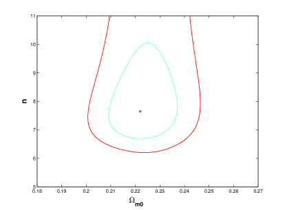
Figure 1: Constraints on $f(T)$ theory with $68.3\%$ and $95.4\%$ confidence regions in the $\Omega_{m0}$-$n$ plane fitted on combinational observation of SNIa, BAO, and CMB data. The blue asterisk is the best-fit point.

In terms of Eq. (3.4), we reconstruct the effective equation of state in Figure 2. We find that $w_{\rm{eff}}(z)$ is a decreasing function of redshift, and steadily approaches to -1 for high redshift $z\gtrsim 1$. That is, the geometric effect behaves like the cosmological constant at early epoch. However, it generally increases with the decrease of redshift. The present value of the effective equation of state finally reaches $w_{\rm{eff0}}=-0.8760$. Moreover, the $w_{\rm{eff}}(z)$ crosses through -1 for $z<1$ within $1\sigma$ confidence level. In Figure 3, we also reconstruct the deceleration parameter $q(z)$. We find that the transition from decelerating to accelerating expansion occurs at $z=0.95\pm 0.05$, which is earlier than some phenomenological deceleration parameters (Riess et al. 2004; Cunha & Lima 2008). With the decrease of deceleration parameter, its value today is $q_{0}=-0.3750$. In the near future $z=-0.04$, the $q(z)$ crosses the zero. That is to say, the accelerating expansion of the universe may be slowing down again and till to decelerating expansion take place in future. It is possible, however, to have an eternal accelerated phase at 68.3% confidence level as shown in Figure 3. The feature of transient acceleration makes this $f(T)$ gravity compatible with the S-matrix description of string theory (Banks & Dine 2001; Hellerman et al. 2001). Most of dark energy models including the current standard $\Lambda$CDM scenario predict an eternally accelerating universe. But the consequent cosmological event horizon dose not allow the construction of a conventional S-matrix to describe particle interactions (Guimaraes & Lima 2011). However, from the standpoint of string theory, the existence of conventional S-matrix is absolutely essential for an asymptotically large space at infinity (Cui et al. 2013). Therefore, S-matrix is ill-defined in an eternal accelerating universe. In order to alleviated the conflict between dark energy and String theory, several dynamic dark energy models have been proposed to achieve the possibility of transient acceleration phenomenon (Cui et al. 2013; Russo 2004; Carvalho et al. 2006a). In addition, recently it was also argued that the SNIa data favors a transient acceleration (Shafieloo et al. 2009)which is not excluded by current observations (Guimaraes & Lima 2011; Vargas et al. 2012; Bassett et al. 2002). Our result indicates that this type of $f(T)$ gravity serves as an alternative from modification of gravity to the dynamic dark energy models.

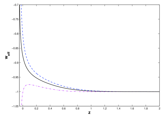
Figure 2: Reconstruction of the effective equation of state at $68.3\%$ confidence level for the $f(T)$ gravity considered here.

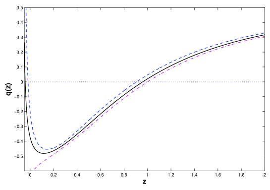
Figure 3: Reconstruction of the deceleration parameter at $68.3\%$ confidence level for the $f(T)$ gravity considered here.

5 Summary and conclusions

The $f(T)$ gravity based on modification of the teleparallel gravity was proposed to explain the accelerating expansion of the universe without the need of dark energy. A brief overview of a specific $f(T)$ gravity proposed in (Yang 2011b) was also given. We also introduced the method used to constrain cosmological models with observational data including SNIa, BAO, and CMB. After constraining the $f(T)$ gravity proposed in (Yang 2011b), we find that the best-fit values of the parameters at the $68.3\%$ confidence level are: $\Omega_{m0}=0.22^{+0.0089}_{-0.0094}$ and $n=7.64^{+1.175}_{-0.67}$ with $\chi^{2}_{\rm min}=579.4786$ ($\chi^{2}_{\rm min}/$dof=0.9923). The parameters $\Omega_{m0}$ and $n$ can be constrained well at $68.3\%$ confidence level by these observational data.

We also reconstructed the effective equation of state and the deceleration parameter from observational data. We found that the transition from deceleration to acceleration occurs at $z=0.95\pm 0.05$. The present value of deceleration parameter was found to be $q_{0}=-0.3750$, meaning that the cosmic expansion has passed a maximum value (about at $z\sim 0.1$) and is now slowing down again. This is a theoretically interesting result because eternally accelerating universe (like $\Lambda$CDM) is endowed with a cosmological event horizon which prevents the construction of a conventional S-matrix describing particle interactions. Such a difficulty has been pointed out as a severe theoretical problem for any eternally accelerated universe (Hellerman et al. 2001; Cline 2001; Carvalho et al. 2006b). Some researches also indicated that a transient phase of accelerated expansion is not excluded by current observations (Guimaraes & Lima 2011; Vargas et al. 2012; Bassett et al. 2002). We note, however, it is possible to have an eternal accelerated phase and an effective equation of state crossing through $-1$ at $68.3\%$ confidence level, according to the reconstruction of the effective equation of state and the deceleration parameter. We look forward to a more comprehensive investigation including the observations of structure growth which is widely used to study $f(T)$ gravity (Izumi & Ong 2013; Chen et al. 2011; Geng & Wu 2013; Zheng & Huang 2011a; Li et al. 2011b), to reduce errors of the effective equation of state and the deceleration parameter at $z\sim 0$.