Detection of vibronic bands of C₃ in a translucent cloud towards HD 169454

Abstract

We report the detection of eight vibronic bands of C₃, seven of which have been hitherto unobserved in astrophysical objects, in the translucent cloud towards HD 169454. Four of these bands are also found towards two additional objects: HD 73882 and HD 154368. Very high signal-to-noise ratio ($\sim$1000 and higher) and high resolving power ($R=80,000$) UVES-VLT spectra (Paranal, Chile) allow for detecting novel spectral features of C₃, even revealing weak perturbed features in the strongest bands. The work presented here provides the most complete spectroscopic survey of the so far largest carbon chain detected in translucent interstellar clouds. High-quality laboratory spectra of C₃ are measured using cavity ring-down absorption spectroscopy in a supersonically expanding hydrocarbon plasma, to support the analysis of the identified bands towards HD 169454. A column density of N(C₃) = $(6.6\pm 0.2)\times 10^{12}$ cm^-2 is inferred and the excitation of the molecule exhibits two temperature components; $T_{exc}=22\pm 1$ K for the low-$J$ states and $T_{exc}=187\pm 25$ K for the high-$J$ tail. The rotational excitation of C₃ is reasonably well explained by models involving a mechanism including inelastic collisions, formation and destruction of the molecule, and radiative pumping in the far-infrared. These models yield gas kinetic temperatures comparable to those found for $T_{exc}$. The assignment of spectral features in the UV-blue range 3793-4054 Å may be of relevance for future studies aiming at unravelling spectra to identify interstellar molecules associated with the diffuse interstellar bands (DIBs).

1 Introduction

Currently, some 180 different molecules have been detected in dense inter- and circumstellar clouds, largely in radio- and submilimeter surveys, with this number growing with several new species per year. However, only about ten simple molecules are observed in the visible part of the electromagnetic spectrum as absorption features originating in translucent clouds, transparent for optical wavelengths. Among them are homonuclear species, such as H₂, C₂ and C₃, which are not accessible to radio observations. Bare carbon chains do not exhibit pure rotational transitions, because of the lack of a permanent dipole moment, and thus only their electronic or vibrational spectral features can be observed. The latter cover the spectral range from the vacuum UV until the far infrared. Determination of the abundances of simple carbon molecules in interstellar clouds is important, as they are considered building blocks for many already known interstellar molecules with a carbon skeleton.

After the $19^{th}$ century discovery of the 4052 Å band in the spectrum of comet Tebbutt (Huggins, 1881) and the assignment of this blue absorption feature to the C₃ molecule (Douglas, 1951), the triatomic carbon chain radical was detected in the circumstellar shell of the star IRC+10216 (Hinkle et al., 1988) and subsequently, albeit tentatively, in the interstellar medium (Haffner & Meyer, 1995). Cernicharo et al. (2000) detected nine lines of the $\nu_{2}$ bending mode towards Sgr B2 and IRC+10216, observed in the laboratory by Giesen et al. (2001). This spectral range is, however, not applicable to observations of translucent clouds. High resolution observations using the Herschel/HIFI instrument detected transitions of C₃ originating in the warm envelopes of massive star forming regions (Mookerjea et al., 2010; Mookerjea et al., 2012); in these environments high densities of $10^{5}-10^{6}$ cm^-3 prevail, whereas in diffuse clouds densities are limited to $10^{3}$ cm^-3. The presence of C₃ in the diffuse interstellar medium was proven by Maier et al. (2001), based on the detection of the Ã${}^{1}\Pi_{u}$–X̃${}^{1}\Sigma_{g}^{+}$ 000–000 band close to 4052 Å towards three reddened stars. Up to now the highest resolution study of C₃ in such environments was reported by Galazutdinov et al. (2002b), although restricted to a few objects only. These observations provided the only reliable estimates so far of the abundance of this molecule, yielding values an order of magnitude below that of C₂. Other observations of C₃ in translucent clouds (Roueff et al., 2002; Ádámkovics et al., 2003; Oka et al., 2003) suffered from lower signal-to-noise ratios, giving rise to large uncertainties in the deduced column densities.

The existing data for linear carbon molecules longer than C₃, like C₄ (Linnartz et al., 2000), or C₅ (Motylewski et al., 1999), fail to provide firm evidence for their existence in the interstellar medium (Galazutdinov et al., 2002a; , 2002, 2004). For a systematic investigation of the conditions under which carbon-based molecules are produced in the interstellar medium, a larger class of targets exhibiting a variety of optical properties and physical conditions in the intervening clouds has to be observed. The targeted objects should be selected for translucent clouds with the carbon-bearing molecules producing a single Doppler-velocity component, thus allowing for an unambiguous analysis of the spectrum, and resulting in accurate column densities.

The identification of the carriers of diffuse interstellar bands (DIBs) remains, since their discovery by Heger (1922), one of the persistently unresolved problems in spectroscopy. The current list of unidentified interstellar absorption features contains more than 400 entries (Hobbs et al., 2008). The presence of substructures inside DIB profiles, discovered by Sarre et al. (1995) and by Kerr et al. (1998), supports the hypothesis of their molecular origin. The established relation between profile widths of DIBs and rotational temperatures of linear carbon molecules (Kazmierczak et al., 2010) makes the latter interesting targets for observations. Both C₂ and C₃ may show different rotational temperatures along different lines of sight, as shown by Ádámkovics et al. (2003). This is associated with the fact that their rotational transitions are forbidden and thus cooling of their internal degrees of freedom is inefficient. For this reason, an accurate determination of rotational excitation temperatures of short carbon chains may help to shed light on the origin of the mysterious carriers of the DIBs (Kazmierczak et al., 2010b).

Observationally, the spectral features originating from either C₂ or C₃ typically turn out to be rather shallow and thus high S/N ratios and high spectral resolution are required to establish accurate values for the excitation temperature. The aim of the present investigation is to use the superior capabilities of UVES-VLT to obtain high quality spectra of C₃. All previous studies were based solely on the strongest 000–000 band of the Ã${}^{1}\Pi_{u}$–X̃${}^{1}\Sigma_{g}^{+}$ electronic system. Here additional vibronic bands in the Ã${}^{1}\Pi_{u}$–X̃${}^{1}\Sigma_{g}^{+}$ electronic system of C₃ are identified along sight lines towards objects HD 169454, HD 73882, and HD 154368. A detailed analysis of eight vibronic bands detected towards the object HD 169454 is presented. The astronomical observations are supported by a high-quality laboratory investigation, using cavity ring-down laser spectroscopy, producing fully rotationally resolved C₃ spectra of the vibronic bands in the ÖX̃ system. The combined information of laboratory and observed spectra is used to deduce column densities and a rotational temperature of C₃ in HD 169454 The results are interpreted in terms of excitation models for C₃ (Roueff et al., 2002) and a chemical model of a translucent cloud towards HD 169454.

2 Methods

2.1 Observations

The observational material, of which a target list is presented in Table 1, was obtained using the UVES spectrograph mounted on the ESO Very Large Telescope at Paranal (Chile) with resolution $R=80,000$ in the blue arm (3020 – 4980 Å) occupying the C₃ bands of interest, as well as CH and CH⁺. The data set comprises spectra acquired during our observation run of March 2009 (program 082.C-0566(A)) and data from the ESO Archive programs 71.C-0367(A) and 076.C-0431(B). The spectra, averaged over 10 - 50 exposures are of exceptionally high S/N ratio with values between 1900-2800.

Table 1: A list of observed targets in which C₃ was detected at 4052 Å with specific physical characteristics and observed signal-to-noise ratio (S/N).

Star	SpL	V	B-V	E(B-V)	S/N
HD 73882	O8V	7.21	+0.40	0.67	$\sim$1900
HD 154368	O9.5Iab	6.14	+0.50	0.73	$\sim$2200
HD 169454	B1Ia	6.62	+0.90	1.11	$\sim$2800

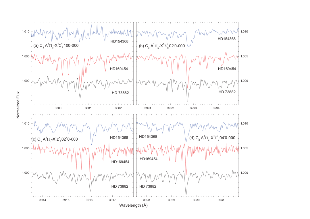
Figure 1: Four vibronic bands in the Ã${}^{1}\Pi_{u}$–X̃${}^{1}\Sigma_{g}^{+}$ system of C₃ observed in HD 154368, HD 169454, and HD 73882, .

All spectra were reduced with the standard IRAF packages, as well as our own DECH code (Galazutdinov, 1992), providing the standard procedures of image and spectra processing. Using different computer codes for data analysis reduces the inaccuracies connected to the slightly different ways of dark subtraction, flat fielding, or excision of cosmic ray hits.

The very high S/N of the spectra allowed us to detect seven ÖX̃ vibronic C₃ bands in addition to the ÖX̃ origin (000-000) band in the spectrum of the heavily reddened star: HD 169454. Four vibronic bands were also detected in sight lines towards HD 73882 and HD 154368. These two sight lines are not analysed in detail in this paper. The resulting spectra for these four bands in all three objects are shown in Fig. 1 and are illustrative for the quality of the observational data. All targets are heavily reddened and characterized by strong molecular features. The individual spectra of identified vibronic bands in the sight line to HD 169454 are presented in Figs. 2 - 9, alongside with the laboratory spectra, in the order of excited vibrations: ${\nu_{1}}{\nu_{2}^{+/-}}{\nu_{3}}$ for symmetric stretching, bending - degenerate-, and asymmetric stretching, respectively, as well as combination modes. In this sequence of figures the laboratory spectra are plotted with blue lines, the astronomical spectra are displayed as black histograms overlayed with a thin line representing a synthetic spectrum based on the detailed analysis. The identification of rotational lines is indicated by vertical lines. In the C₃ Ã${}^{1}\Pi_{u}$– X̃${}^{1}\Sigma_{g}^{+}$ 000–000 band, see Fig. 2, a series of perturber lines is observed, confirming findings of a laboratory study by Zhang et al. (2005). These perturber features are marked with additional thin vertical lines in Fig. 2.

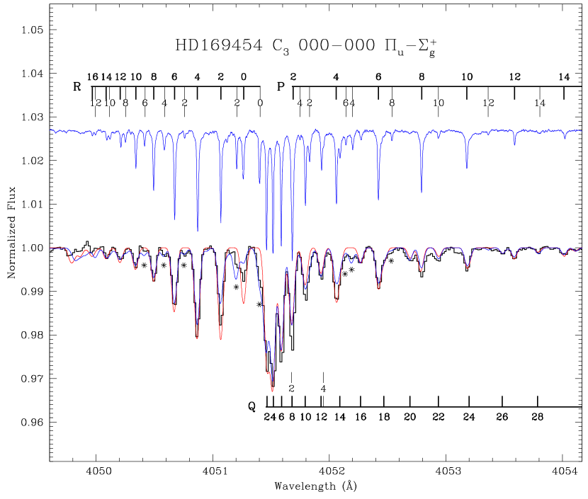
Figure 2: Spectrum of the C₃ Ã${}^{1}\Pi_{u}$ - X̃${}^{1}\Sigma_{g}^{+}$ 000–000 band. Upper spectrum: laboratory measurement by cavity ring-down spectroscopy in a planar plasma jet. Lower spectrum: observation in the sight line to HD 169454. Positions of rotational lines are tagged with thick lines. Thin lines tag rotational lines due to perturbing states based on the analysis of Zhang et al. (2005). The astronomical spectrum is overlaid with fitted curves: the red curve represents a fit using only unperturbed lines; for the blue curve perturber lines are included in the fit. Note the remaining deviation for the intensity of the R(0) line in the simulated spectrum (see text).

For the detailed analysis of the vibronic bands in the sight line to HD 169454 the spectrum was shifted to the rest wavelength velocity frame using the CH A-X and B-X lines. Redshifts as large as 0.85 km s^-1 were observed in the case of CN B-X (0,0) lines and 2.8 km s^-1 in the case of the Ca I 4226.7 Å line. While fitting individual bands some shifts in wavelengths are necessary, mostly consistent with velocities of the CN lines.

2.2 Laboratory experiment

Laboratory spectra of C₃ are recorded in direct absorption using cavity ring-down laser spectroscopy. Details of the experimental setup and experimental procedures can be found elsewhere (Zhao et al., 2011; Motylewski & Linnartz, 1999). Briefly, in the current experiment, supersonically jet-cooled C₃ radicals are produced in a pulsed (10 Hz) planar plasma expansion generated by discharging 0.5% C₂H₂ diluted in a 1:1 helium/argon gas mixture. A 3 cm $\times$ 300 $\mu$m slit discharge nozzle is employed to generate a planar plasma expansion which provides an essentially Doppler-free environment and a relatively long effective absorption path length. The rotational temperature of C₃ in the plasma jet is estimated at 30 K.

Tunable violet light (375 - 410 nm) is generated by frequency-doubling the near infrared output (750 - 820 nm) of a Nd:YAG-pumped pulsed dye laser ($\sim$6 ns pulse duration). The bandwidth of the violet laser pulses is  0.06 cm^-1. Since this value exceeds the Doppler width ($<$0.03 cm^-1) of C₃ transitions in the plasma jet, the absolute line intensities in the recorded spectrum may be underestimated, due to a specific linewidth effect associated with the cavity ring-down technique. This effect (Jongma et al., 1995) is small in the case of weak absorptions but may become pronounced in the case of strong absorptions. Therefore, in the present experiment, production densities of C₃ in the plasma are controlled to be not too high, ensuring reliable line intensities for each individual band, to derive accurate values from the experimental spectra (Haddad et al., 2014).

Simultaneously with the spectral recordings of C₃, transmission fringes of two etalons (with free spectral ranges of $\sim$20.1 and 7.57 GHz, respectively) are recorded at the fundamental infrared laser wavelength, providing relative frequency markers to correct for possible non-linear wavelength scanning of the dye laser. The absolute laser frequency is calibrated by absorption lines of He I or Ar I in the plasma. In this way, a wavelength accuracy of better than 0.01 Å is achieved in the final laboratory spectrum, except for the 02⁺0 – 000 band at $\sim$3916 Å, around which no strong He I or Ar I lines are found. The laboratory spectrum of this 02⁺0 – 000 band is calibrated by using the wavelength of the strongest C₃ transition, i.e. Q(4) line at 3916.05 Å, in the astronomical spectrum towards HD 169454. This yields an absolute wavelength accuracy of $\sim$0.05 Å for the 02⁺0 – 000 band, while the accuracy of relative line positions within this band is better than 0.01 Å.

These data sets are used to build a C₃ line list, as is discussed in the next section.

3 Molecular data

The vibronic bands in the Ã${}^{1}\Pi_{u}$– X̃${}^{1}\Sigma_{g}^{+}$ electronic system of C₃ have been previously investigated in the laboratory by Gausset et al. (1965); Balfour et al. (1994); Tokaryk & Chomiak (1997); McCall et al. (2003); Tanabashi et al. (2005); Zhang et al. (2005); Chen et al. (2010). Most studies were performed at lower spectral resolution and consequently lower wavelength precision than the data presented here. The present laboratory spectra, combined with the previously reported data, allow us to build a highly precise line list for C₃. Tables 3 – 5 summarize the list of laboratory line positions, details of which are given in the subsections below.

3.1 ÖX̃ oscillator strength and Franck-Condon factors

In our analysis we rely on the determination of the oscillator strength from a measurement of the lifetime of the upper electronic state Ã${}^{1}\Pi_{u}$ corresponding to a value of $f_{el}=0.0246$ (Becker et al., 1979). With a calculation of the Franck-Condon factor (FCF) for the 000–000 band (Radić-Perić et al., 1977) yielding 0.74, this translates approximately to $f_{000}=0.016$, a value previously used in the analyses of interstellar C₃ by Maier et al. (2001), Ádámkovics et al. (2003), and Oka et al. (2003). Computations of FCFs carried out by Jungen & Merer (1980) in an effective large amplitude formalism lead to 15 percent lower value of $f_{000}=0.0146$ used by Roueff et al. (2002). Our choice is dictated by easy comparison to earlier determinations of C₃ column densities in sight line to HD 169454 in light of uncertainty of the FCF value.

Interpretation of the other band intensities requires knowledge of the Franck-Condon factors for individual vibronic bands. Calculation of FCFs is hampered by the occurrence of low-frequency and large-angle bending modes, as well as by perturbations in the Ã${}^{1}\Pi_{u}$ state, which affects the ÖX̃ electronic transition moment as well as the FCFs. Computations of FCFs were carried out by Jungen & Merer (1980) in an effective large amplitude formalism for the transitions involving bending modes. Calculations performed by Radić-Perić et al. (1977) resulted in different FCF values. The intensities in the astronomical spectra were used to experimentally determine FCFs as well. For this purpose the intensities for R(0), R(2), R(4) and R(6) transitions, most easily identifiable, except in the 120-000 band, were used, and normalized to the value of $f_{000}=0.016$ of Radić-Perić et al. (1977) adopted in this paper. A summary of available FCFs from the two theoretical studies and the presently determined experimental values is listed in Table 2. The experimentally determined values, that agree in most cases with the average of both theoretical studies, are used for producing the line strengths included in the molecular line lists in Tables 3 – 5.

Table 2: Franck-Condon factors of the analysed vibronic bands.

Origin	Band	FC			References
(Å)		J&M	R-P	this work
4051.6	000 $\Pi_{u}$	0.594	0.741	0.741	1,2
3880.7	100 $\Pi_{u}$			0.13$\pm$0.02	2
3992.8	02-0 $\Pi_{u}$	0.087	0.170	0.14$\pm$0.03	3
3916.0	02+0 $\Pi_{u}$	0.081	0.170	0.14$\pm$0.03	2
3929.5	04-0 $\Pi_{u}$	0.083	0.056	0.10$\pm$0.03	2
3801.7	04+0 $\Pi_{u}$	0.048	0.056	0.10$\pm$0.03	4
3794.2	002 $\Pi_{u}$			0.08$\pm$0.02	4
3826.0	12-0 $\Pi_{u}$			0.04$\pm$0.01	2,5

J&M Jungen & Merer (1980); R-P Radić-Perić et al. (1977); References: (1) Zhang et al. (2005); (2) This work; (3) Tokaryk & Chomiak (1997); (4) Gausset et al. (1965); (5) Chen et al. (2010).

Because all bands have a $\Pi$ ($K=1$) upper vibronic state and a $\Sigma$ ($K=0$) lower ground state, the Hönl-London factors for these bands, for $\Delta K=1$ (corresponding to both $\Delta l=0$ and $\Delta l=2$) are: $1/2(J+2)/(2J+1)$, $1/2$, and $1/2(J-1)/(2J+1)$ for R, Q, and P-branch transitions, respectively. The heavily perturbed 000-000 band requires a more sophisticated treatment, as is discussed below.

3.2 ÖX̃ 000-000 band at 4050 Å

The origin band has been analyzed in detail in various laboratory investigations (Gausset et al., 1965; Zhang et al., 2005; McCall et al., 2003; Tanabashi et al., 2005). Earlier indications of a misassigned R(0) transition were clarified and a number of extra transitions was identified by McCall et al. (2003). Zhang et al. (2005) proposed an explanation for the existence of extra transitions via intensity borrowing to two perturbing states lying close to the upper Ã${}^{1}\Pi_{u}$ 000 state, and presented an effective Hamiltonian for the upper Ã${}^{1}\Pi_{u}$ 000 state. The laboratory spectrum for this band, shown in Fig. 2, agrees reasonably well with previous work, and provides more reliable line intensities for the sight line spectrum towards HD 169454, particularly for the weaker transitions and transitions involving perturbing states. Using the new laboratory data it was possible to improve the Hamiltonian significantly, and the perturbed components are now better reproduced. Note that some perturbed transitions are positively identified in the astronomical spectra - see transitions marked with an asterisk in Fig. 2. Still, in this perturbation analysis there remains a discrepancy for the R(0) line, as is clearly seen in the simulated spectrum, shown in Fig. 2. For the R(0) line there is a nearly equal mixture between singlet and triplet character with an indication of an additional perturbation for the very lowest $J$-value, not addressed previously. Oscillator strengths obtained from this new analysis together with derived column densities are presented in Table 3. However, data for the R(0) and P(2) lines of this band are not used for deriving column densities, in view of the severe perturbations in the $J=1$ excited level and the deviations still present in the modeling in this part of the spectrum (cf. Fig. 2). For $J>20$ the values are taken from Tanabashi et al. (2005).

Because of the remaining discrepancies, we propose the following approach to deal with intensities of perturbed components. Under the assumption of a single electronic transition moment, perturbed components related to a high vibrational level of the b̃${}^{3}\Pi_{g}$ state borrow intensity from the Ã-X̃ transition. Summing over equivalent widths of regular and perturbed components, column densities can be derived for the Ã-X̃ 000-000 band using line intensities neglecting effects of perturbations. The corresponding oscillator strengths are then based on the Hönl-London factors and presented in Table 4 with wavelengths of regular components. This approach is finally used in the determination of column densities in Section 4.

3.3 ÖX̃ 100-000 band at 3881 Å

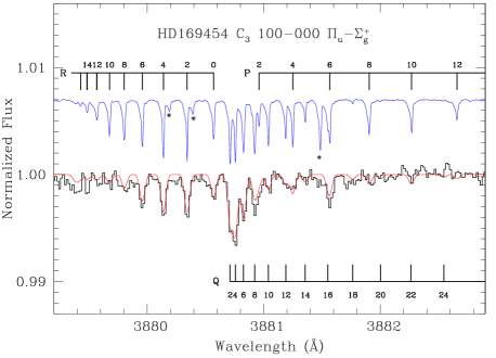
Figure 3: Laboratory spectrum (blue line) and astronomical spectrum in the sight line to HD 169454 (black) for the C₃ Ã${}^{1}\Pi_{u}$ - X̃${}^{1}\Sigma_{g}^{+}$ 100-000 band. A synthetic spectrum overplots the observed spectrum with a red line. Positions of rotational lines are indicated with vertical lines. Note the presence of additional lines marked by (*) in the laboratory spectrum (see text).

A line list for the 100-000 band is deduced from the present laboratory spectrum, shown in Fig. 3, providing line positions at an accuracy better than 0.01 Å. The line list is extended by transitions not observed in the laboratory spectrum by the following procedure. First, the observed lines are used for the determination of spectroscopic constants of the upper state, fixing the spectroscopic constants of the X̃ ground state to values derived by Tanabashi et al. (2005). The evaluated spectroscopic constants of the à 100 upper state are then used for extending the line list for $J$ up to 50. The residuals between experimental and predicted line positions are in general at the level of 0.01 Å. The laboratory spectrum contains three extra lines, which are not indicative for a perturbation, but rather due to another unknown species present in the plasma expansion, as cavity ring down is not mass selective. These features do not appear in the spectrum of HD 169454.

3.4 ÖX̃ 02^-0 – 000 band at 3993 Å

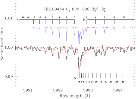
Figure 4: Laboratory spectrum (blue line) and astronomical spectrum in the sight line to HD 169454 (black) for the C₃ Ã${}^{1}\Pi_{u}$ - X̃${}^{1}\Sigma_{g}^{+}$ 02^-0 – 000 band.

The line positions from Tokaryk & Chomiak (1997), the most accurate analysis of this band up to now, agree well with our laboratory data, shown in Fig. 4. Earlier laboratory work by Gausset et al. (1965) and Balfour et al. (1994) suffered from low resolution and most probably from contamination by 020-020 emission bands, resulting in misassignments of some rotational lines. Consistency between our spectrum towards HD 169454 and the laboratory spectrum further strengthens the assignments by Tokaryk & Chomiak (1997).

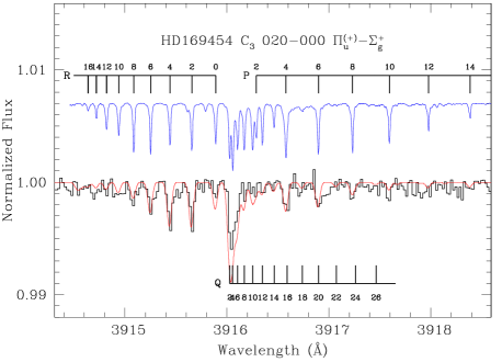
Figure 5: Laboratory spectrum (blue line) and astronomical spectrum in the sight line to HD 169454 (black) for the C₃ Ã${}^{1}\Pi_{u}$ - X̃${}^{1}\Sigma_{g}^{+}$ 02⁺0 – 000 band.

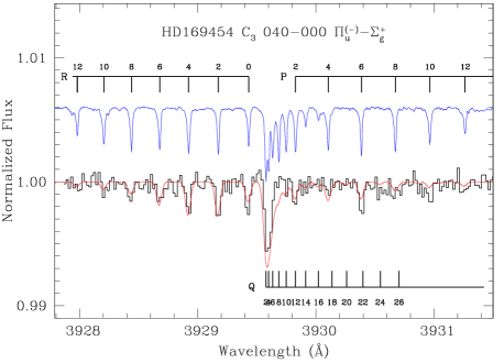
Figure 6: Spectrum in sight line to HD 169454 (black) and laboratory spectrum (blue line) for the C₃ Ã${}^{1}\Pi_{u}$ - X̃${}^{1}\Sigma_{g}^{+}$ 04^-0 – 000 band.

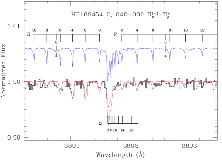
Figure 7: Spectrum in sight line to HD 169454 (black) and laboratory spectrum (blue line) of the C₃ Ã${}^{1}\Pi_{u}$ - X̃${}^{1}\Sigma_{g}^{+}$ 04⁺0 – 000 band. Perturber lines are marked with (*); see text.

Figure 8: Spectrum in sight line to HD 169454 (black) and laboratory spectrum (blue line) of the C₃ Ã${}^{1}\Pi_{u}$ - X̃${}^{1}\Sigma_{g}^{+}$ 002-000 band.

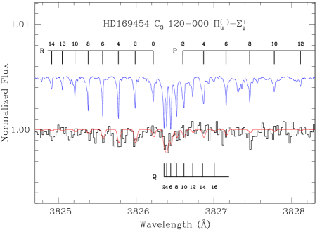
Figure 9: Spectrum in sight line to HD 169454 (black) and laboratory spectrum (blue line) of the C₃ Ã${}^{1}\Pi_{u}$ - X̃${}^{1}\Sigma_{g}^{+}$ 120 – 000 band.

3.5 ÖX̃ 02⁺0 — 000 band at 3916 Å

Entries for the line list are taken from the present laboratory spectrum, shown in Fig. 5, and extended to higher-$J$ transitions based on the deduced molecular constants. As the absolute wavelength calibration relies on the observational spectrum towards HD 169454, the wavelength positions in this band are of a lower accuracy, at the level of $\sim 0.05$ Å.

3.6 ÖX̃ 04^-0 – 000 band at 3930Å

The line list is extracted from the present laboratory data, shown in Fig. 6, and extended to higher-$J$ transitions. Previously reported data by Gausset et al. (1965) and Balfour et al. (1994) do not reproduce the observed spectrum in a consistent manner, likely for misassign as explained in Section 3.4.

3.7 ÖX̃ 04⁺0 – 000 band at 3802 Å

The line list is extracted from the present laboratory data, shown in Fig. 7. Extra lines in the laboratory spectrum marked with an asterisk (*) are associated with perturbation features; based on combination differences these extra lines are assigned as R(6) and P(8) lines.

3.8 ÖX̃ 002-000 band at 3794 Å

The line list is extracted from the laboratory data shown in Fig. 8. Spectroscopic constants for the upper state are derived, yielding more accurate values than in Chen et al. (2010). Large residuals of $\sim$0.05 Å are found indicating perturbations in the upper state for $J>14$ transitions. Therefore, the line list of this band is not extended beyond this $J$ value.

3.9 ÖX̃ 120 – 000 band at 3826 Å

The line list for this band is extracted from the laboratory data. Due to its weakness, this band is barely visible towards HD 169454. However the detection of this band, based on the low-$J$ Q branch lines clearly visible in Fig. 9, is certain. The quality of the data is not of sufficient accuracy to determine line strengths or column densities.

The line lists providing the C₃ molecular data are presented in Table 3 for the Ã-X̃ 000-000 band taking into account effect of perturbations, in Table 4 for regular transitions only, and in Table 5 for the vibronic bands probing excited vibrations in the upper state, with exception of the 120-000 band system. For a full list of laboratory line positions of the Ã-X̃ 000-000 band and a more detailed account of the perturbation analysis we refer to Haddad et al. (2014).

Table 3: The C₃ line list for the Ã-X̃ 000-000 band as obtained from the present analysis. Perturber lines are marked with an asterisk (*).

Wavelength	Line	$f_{JJ}$	EW	Ncol
(Å)		($\times$103)	(mÅ)	(1012 cm-2)
4050.075	R(14)	3.49	0.10$\pm$0.03	0.20$\pm$0.06
4050.191	R(12)	3.58	0.16$\pm$0.03	0.31$\pm$0.06
4050.327	R(10)	3.73	0.21$\pm$0.03	0.39$\pm$0.06
4050.401*	R(6)	0.58	0.03$\pm$0.02	0.36$\pm$0.24
4050.484	R(8)	3.95	0.37$\pm$0.04	0.65$\pm$0.07
4050.567*	R(4)	0.49	0.08$\pm$0.03	1.12$\pm$0.42
4050.661	R(6)	4.21	0.74$\pm$0.07	1.21$\pm$0.11
4050.746*	R(2)	0.45	0.08$\pm$0.04	1.22$\pm$0.61
4050.857	R(4)	4.44	1.06$\pm$0.11	1.64$\pm$0.17
4051.055	R(2)	3.78	0.96$\pm$0.10	1.75$\pm$0.18
4051.190*	R(2)	2.08	0.22$\pm$0.05	0.73$\pm$0.17
4051.255	R(0)	4.22	0.41$\pm$0.08
4051.396*	R(0)	10.58	0.36$\pm$0.12
4051.448	Q(2)	6.87	1.35$\pm$0.26	1.35$\pm$0.26
4051.506	Q(4)	7.70	1.76$\pm$0.36	1.57$\pm$0.32
4051.578	Q(6)	7.89	1.44$\pm$0.28	1.26$\pm$0.24
4051.782	Q(10)	7.96	0.64$\pm$0.14	0.55$\pm$0.12
4051.820	P(2)	1.06	0.14$\pm$0.07
4051.918	Q(12)	7.97	0.38$\pm$0.06	0.33$\pm$0.05
4052.045	P(4)	1.57	0.56$\pm$0.14	2.45$\pm$0.61
4052.077	Q(14)	7.98	0.27$\pm$0.07	0.23$\pm$0.06
4052.122*	P(6)	0.28	0.09$\pm$0.04	2.21$\pm$0.98
4052.180*	P(4)	0.86	0.15$\pm$0.04	1.20$\pm$0.32
4052.257	Q(16)	7.98	0.20$\pm$0.03	0.17$\pm$0.03
4052.412	P(6)	2.56	0.49$\pm$0.08	1.32$\pm$0.22
4052.459	Q(18)	7.99	0.13$\pm$0.08	0.11$\pm$0.07
4052.521*	P(8)	0.39	0.06$\pm$0.03	1.06$\pm$0.53
4052.683	Q(20)	7.99	0.20$\pm$0.08	0.17$\pm$0.07
4052.782	P(8)	2.82	0.40$\pm$0.08	0.98$\pm$0.20
4053.169	P(10)	2.87	0.30$\pm$0.04	0.72$\pm$0.10
4053.479	Q(26)	7.99	0.08$\pm$0.03	0.07$\pm$0.03
4053.577	P(12)	2.87	0.14$\pm$0.05	0.34$\pm$0.12
4053.783	Q(28)	8.00	0.05$\pm$0.03	0.04$\pm$0.03
4054.005	P(14)	2.86	0.09$\pm$0.03	0.22$\pm$0.07

Table 4: The C₃ line list for the Ã-X̃ 000-000 band as obtained from unperturbed intensities only.

Wavelengtha	Line	$f_{JJ}$	EW	Ncol
(Å)		($\times$103)	(mÅ)	(1012 cm-2)
4050.075	R(14)	4.41	0.10$\pm$0.03	0.16$\pm$0.05
4050.191	R(12)	4.48	0.16$\pm$0.03	0.25$\pm$0.05
4050.327	R(10)	4.57	0.21$\pm$0.03	0.32$\pm$0.05
4050.484	R(8)	4.72	0.37$\pm$0.04	0.54$\pm$0.06
4050.661	R(6)	4.92	0.77$\pm$0.09	1.08$\pm$0.13
4050.857	R(4)	5.33	1.14$\pm$0.14	1.47$\pm$0.18
4051.055	R(2)	6.40	1.26$\pm$0.19	1.36$\pm$0.20
4051.396	R(0)	16.00	0.77$\pm$0.20	0.33$\pm$0.09
4051.448	Q(2)	8.00	1.35$\pm$0.26	1.16$\pm$0.22
4051.506	Q(4)	8.00	1.76$\pm$0.36	1.51$\pm$0.31
4051.578	Q(6)	8.00	1.44$\pm$0.28	1.24$\pm$0.24
4051.782	Q(10)	8.00	0.64$\pm$0.14	0.55$\pm$0.12
4051.918	Q(12)	8.00	0.38$\pm$0.06	0.33$\pm$0.05
4052.045	P(4)	2.67	0.71$\pm$0.18	1.83$\pm$0.46
4052.077	Q(14)	8.00	0.27$\pm$0.07	0.23$\pm$0.06
4052.257	Q(16)	8.00	0.20$\pm$0.03	0.17$\pm$0.03
4052.412	P(6)	2.56	0.58$\pm$0.12	1.56$\pm$0.32
4052.459	Q(18)	8.00	0.13$\pm$0.08	0.11$\pm$0.07
4052.683	Q(20)	8.00	0.20$\pm$0.08	0.17$\pm$0.07
4052.782	P(8)	3.29	0.46$\pm$0.11	0.96$\pm$0.23
4053.169	P(10)	3.43	0.30$\pm$0.04	0.60$\pm$0.08
4053.479	Q(26)	8.00	0.08$\pm$0.03	0.07$\pm$0.03
4053.577	P(12)	3.52	0.14$\pm$0.05	0.27$\pm$0.10
4053.783	Q(28)	8.00	0.05$\pm$0.03	0.04$\pm$0.03
4054.005	P(14)	3.59	0.09$\pm$0.03	0.17$\pm$0.06

^a wavelengths of the regular components

Table 5: The C₃ line list for transitions to excited vibrational levels in the à state.

Wavelength	Line	$f_{JJ}$	EW	Ncol
(Å)		($\times$103)	(mÅ)	(1012 cm-2)
100-000
3879.797	R(8)	0.83	0.09$\pm$0.04	0.81$\pm$0.36
3879.952	R(6)	0.87	0.16$\pm$0.03	1.38$\pm$0.26
3880.132	R(4)	0.93	0.18$\pm$0.03	1.45$\pm$0.24
3880.336	R(2)	1.13	0.18$\pm$0.03	1.20$\pm$0.20
3880.563	R(0)	2.82	0.11$\pm$0.03	0.29$\pm$0.08
3880.705	Q(2)	1.41	0.21$\pm$0.03	1.12$\pm$0.16
3880.750	Q(4)	1.41	0.33$\pm$0.03	1.76$\pm$0.16
3880.820	Q(6)	1.41	0.20$\pm$0.03	1.06$\pm$0.16
3880.916	Q(8)	1.41	0.17$\pm$0.03	0.90$\pm$0.16
3880.953	P(2)	0.28	0.08$\pm$0.03	2.14$\pm$0.80
3881.034	Q(10)	1.41	0.07$\pm$0.03	0.37$\pm$0.16
3881.182	Q(12)	1.41	0.06$\pm$0.03	0.32$\pm$0.16
3881.243	P(4)	0.47	0.07$\pm$0.03	1.12$\pm$0.48
02-0 – 000
3991.620	R(8)	0.93	0.12$\pm$0.03	0.92$\pm$0.23
3991.840	R(6)	0.97	0.16$\pm$0.03	1.17$\pm$0.22
3992.070	R(4)	1.05	0.24$\pm$0.03	1.62$\pm$0.20
3992.317	R(2)	1.26	0.20$\pm$0.04	1.13$\pm$0.23
3992.575	R(0)	3.15	0.14$\pm$0.03	0.32$\pm$0.07
02+0-000
3915.080	R(8)	0.92	0.11$\pm$0.03	0.88$\pm$0.24
3915.246	R(6)	0.96	0.15$\pm$0.03	1.15$\pm$0.23
3915.435	R(4)	1.04	0.22$\pm$0.03	1.56$\pm$0.21
3915.649	R(2)	1.25	0.21$\pm$0.03	1.24$\pm$0.18
3915.884	R(0)	3.13	0.07$\pm$0.03	0.16$\pm$0.07
3916.573	P(4)	0.53	0.14$\pm$0.03	1.95$\pm$0.42
3916.890	P(6)	0.61	0.13$\pm$0.04	1.57$\pm$0.48
3917.225	P(8)	0.64	0.09$\pm$0.03	1.04$\pm$0.35
04-0 – 000
3928.433	R(8)	0.62	0.08$\pm$0.03	0.94$\pm$0.35
3928.672	R(6)	0.65	0.10$\pm$0.04	1.13$\pm$0.45
3928.917	R(4)	0.71	0.12$\pm$0.03	1.24$\pm$0.31
3929.168	R(2)	0.85	0.15$\pm$0.04	1.29$\pm$0.34
3929.425	R(0)	2.11	0.12$\pm$0.03	0.42$\pm$0.10
04+0 – 000
3801.021	R(4)	0.72	0.15$\pm$0.02	1.63$\pm$0.22
3801.239	R(2)	0.87	0.13$\pm$0.03	1.17$\pm$0.27
3801.485	R(0)	2.17	0.06$\pm$0.03	0.22$\pm$0.11
002 – 000
3793.734	R(8)	0.48	0.10$\pm$0.04	1.64$\pm$0.65
3793.864	R(6)	0.51	0.15$\pm$0.04	2.31$\pm$0.62
3794.030	R(4)	0.55	0.20$\pm$0.10	2.85$\pm$1.43
3794.215	R(2)	0.66	0.13$\pm$0.03	1.55$\pm$0.36
3794.426	R(0)	1.66	0.04$\pm$0.03	0.19$\pm$0.14
3794.567	Q(2)	0.84	0.16$\pm$0.04	1.49$\pm$0.37
3794.616	Q(4)	0.84	0.10$\pm$0.03	0.93$\pm$0.28
3794.689	Q(6)	0.84	0.11$\pm$0.03	1.03$\pm$0.28
3794.918	Q(10)	0.84	0.14$\pm$0.07	1.31$\pm$0.65
3795.081	P(4)	0.27	0.07$\pm$0.03	2.03$\pm$0.87

Figure 10: Information on column densities in HD 169454, as derived from seven vibronic bands in the Ã-X̃ system of C₃, presented as Boltzmann plots. Note that the limited energy range of the diagram chosen for better illustration of all seven bands resulted in absence of the higher rotational levels in the 000-000 band.

4 Data analysis; column densities

Equivalent widths of rotationally resolved lines in vibronic bands of the C₃ Ã-X̃ system have been measured using DECH and independently with the deblend task of the IRAF package. Errors of equivalent widths were based on a noise model with constant Gaussian width taken from a measured S/N estimated at 2000. When tracing of the continuum was dubious, a systematic error was added. Further, in case of blends, or broad absorptions underlying spectral lines, the full width at half maximum (FWHM) of a Gaussian profile was fixed to the value of the instrumental width (0.051 Å) for the astronomical observations (corresponding to $R=80,000$). This value for the FWHM of the instrumental profile is confirmed by the best fits to clean absorbing lines. The C₃ line positions were found to be systematically redshifted by a value comparable or smaller than the accuracy of the laboratory measurements, 0.01 Å, corresponding to a maximal redshift of 0.8 km s^-1.

Observations of C₂ in the sight line to HD 169454 with the Ultra High Resolution Facility (Crawford, 1997) indicated the existence of at least two velocity components present in the intervening diffuse cloud. Yet, the components are barely resolved and a possible splitting has been ignored in our analysis. Since the C₃ lines in the present study are relatively weak, W${}_{\lambda}\leq 2$ mÅ, column densities of C₃ can be deduced assuming the cloud to be optically thin, so that the total column density is equal to the sum of those of the velocity components. This assumption may influence the final excitation temperatures but does not affect the observed column densities.

Column densities of the X̃ ground state levels for each quantum number $J$ are derived from the equivalent widths and based on the line lists of Tables 4 and 5. Note that the equivalent widths in Table 4 are sum of regular and perturbed components available from Table 3. The resulting column densities are listed in Table 6 for each band separately. The last column contains the weighted average of all analysed bands. The one-but-last row of Table 6 shows column densities summed over the observed transitions in each separate band. The derived column densities, listed in Table 6, are presented in the form of Boltzmann plots for individual bands in Fig. 10, up to $J=18$. An extended Boltzmann plot for the weighted average column densities of the analysed Ã-X̃ bands, including higher $J$ levels solely dependent on the Ã-X̃ 000-000 band, is presented in Fig. 11. In such plots the negative inverse of the slope of the straight line is equal to the excitation temperature. For each band we show the least square fit for the lowest $J=0,2,4,6$ rotational levels and the resulting value of the excitation temperature. The distribution of the column densities shows a characteristic ”two-temperature” behaviour, as was also found in previous studies (e.g., Maier et al. (2001), see their Fig. 5).

Table 6: Column densities for C₃ quantum states in individual vibronic bands and weighted average of all vibronic bands.

$J$	Energy	Ncol
	(cm-1)	(1012 cm-2)
		000 – 000	100 – 000	02-0 – 000	02+0 – 000	04-0 – 000	04+0 – 000	002 – 000	all bandsa
0	0.0000	0.33$\pm$0.09	0.29$\pm$0.08	0.32$\pm$0.07	0.16$\pm$0.07	0.42$\pm$0.10	0.22$\pm$0.11	0.19$\pm$0.14	0.28$\pm$0.03
2	2.5835	1.27$\pm$0.15	1.17$\pm$0.12	1.13$\pm$0.23	1.24$\pm$0.18	1.29$\pm$0.34	1.17$\pm$0.27	1.52$\pm$0.26	1.23$\pm$0.07
4	8.6112	1.52$\pm$0.15	1.62$\pm$0.13	1.62$\pm$0.20	1.64$\pm$0.19	1.24$\pm$0.31	1.63$\pm$0.22	1.10$\pm$0.26	1.55$\pm$0.07
6	18.0822	1.16$\pm$0.11	1.15$\pm$0.14	1.17$\pm$0.22	1.23$\pm$0.21	1.13$\pm$0.45		1.25$\pm$0.26	1.17$\pm$0.07
8	30.9950	0.57$\pm$0.06	0.89$\pm$0.15	0.92$\pm$0.23	0.93$\pm$0.20	0.94$\pm$0.35		1.64$\pm$0.65	0.65$\pm$0.05
10	47.3475	0.40$\pm$0.04	0.37$\pm$0.16					1.31$\pm$0.65	0.40$\pm$0.04
12	67.1372	0.28$\pm$0.03	0.32$\pm$0.16						0.28$\pm$0.03
14	90.3612	0.18$\pm$0.03							0.18$\pm$0.03
16	117.0160	0.17$\pm$0.03							0.17$\pm$0.03
18	147.0976	0.11$\pm$0.07							0.11$\pm$0.07
20	180.6020	0.17$\pm$0.07							0.17$\pm$0.07
22	217.5244
24	257.8600
26	301.6039	0.07$\pm$0.03							0.07$\pm$0.03
28	348.7507	0.04$\pm$0.03							0.04$\pm$0.03
Obs. Ncol		6.27$\pm$0.28	5.81$\pm$0.36	5.15$\pm$0.44	5.20$\pm$0.39	5.02$\pm$0.74	3.01$\pm$0.36	7.00$\pm$1.04	6.31$\pm$0.18
Tot. Ncola		6.57$\pm$0.29							6.61$\pm$0.19

^a see text for explanation

To assess the quality of the analysis and line lists we have performed a simulation of all observed bands based on the obtained parameters for the column densities and the excitation temperature. Synthetic spectra are computed, assuming an instrumental FWHM of 0.051 Å, and included in Figs. 2-9 as a thin red line. Inspection of the eight vibronic bands observed toward HD 169454 (see Figs. 2-9) shows that intensities in the Q-branch are slightly overestimated in spectra of the bending modes. When using line lists compiled from literature data, this caused a serious problem, particularly in the case of the 04⁺0-000 band, where the best fit to the R branch overestimated the Q band intensity at least twice. With the newly composed line lists (Tables 3 and 5) these discrepancies vanished, suggesting that the origin of the inconsistencies were in erroneous assignments of the lines, and/or improper treatment of perturbations in the spectra.

The excitation temperature of the lowest levels is expected to be close to the gas kinetic temperature in analogy to the excitation model for C₂ (van Dishoeck & Black, 1982). The information of the weighted average column densities of all bands is used to derive an accurate excitation temperature. The low-$J$ rotational lines of the Ã-X̃ 000-000 band are strongly perturbed, but using the procedure of summation of equivalent widths of regular and perturbed transitions we believe to have reduced significantly the effect of unknown intensities of individual components. The excitation temperature of the lowest $J=0,2$, $4$, and $6$ levels determined from the best fit is found to be $22.4^{+1.0}_{-0.9}$ K. The excitation temperature of the high-$J$ tail is $187^{+25}_{-19}$ K (see also Fig. 11).

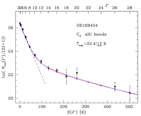
Figure 11: Column density distribution of C₃ X${}^{1}\Sigma_{g}^{+}$ 000 rotational levels towards HD 169454 derived from observations of the Ã-X̃ bands. The dashed line shows the thermal population at 22.4 K obtained from the weighted linear fit to levels $J=0,2,4,6$. The solid red and blue lines show the predictions of the excitation models described in the text.

For the determination of the total column density an estimate for the population of the unobserved levels must be invoked. This is accomplished by fitting the observed average column densities with the analytical formula

$$\ln\frac{\mathrm{N}_{col}(J)}{2J+1}=a\exp(-E(J)/b)+c+d\,E(J),$$ (1)

where $E$ is the excitation energy of level $J$, and $a$, $b$, $c$ and $d$ are free parameters. The population of the lowest $J=0,2,4,6,8$ levels is represented by a linear fit corresponding to an excitation temperature of 22.4 K. Using this approach we have computed the total C₃ column densities (see the last row of Table 6) resulting in a value of N${}_{col}=(6.61\pm 0.19)\times 10^{12}$ cm^-2 for the weighted average over all bands.

The differences between the column densities determined for the individual bands is representative for the overall quality of our data and the procedures followed. The total column density concluded from the weighted average of all bands is shown in Table 7 as a value representative for C₃ along with column densities for other species.

From the present observations it is also possible to deduce a CH column density toward HD 169454 from the lowest Q and R lines in the B-X violet band at 3886.409 and 3890.217 Å, probing both lowest-$J$ $\Lambda$-doublet components, under the assumption that the lines are optically thin. The column density of CH⁺ toward HD 169454 is obtained from the 3597 Å transition in the A-X (1,0) band. The resulting values are included in Table 7.

Table 7: Summary of observed molecular column densities towards HD 169454.

Molecule	Ncol	Texc	Source
	($10^{12}$ cm-2)	(K)
C2	65$\pm$1	19$\pm$2	1
	73$\pm$14	15${}^{+10}_{-5}$	2
	70$\pm$14		3
	160$\pm$29		4
C3	6.61$\pm$0.19	22.4$\pm$1.0	5
	2.24$\pm$0.66a	23.4$\pm$1.4	4
	4.5$\pm$0.3b		3
CH	39.6$\pm$0.3c		5
	46$\pm$8		2
	36.5${}^{+12.6}_{-7.8}$		6
CH+	20.8$\pm$0.2e		5
H2	(8$\times$1020d)		5

^a based on a sample of rotational lines with $J\leq 8$;
^b based on unresolved rotational lines;
^c based on CH line at 3886.409 Å;
^d based on correlation of CH w.r.t. H₂ (Weselak et al. (2004); Fig. 3. therein);
^e based on the CH⁺ line at 3957 Å.
Source: (1) Kazmierczak et al. (2010); (2) Jannuzi et al. (1988); (3) Oka et al. (2003); (4) Ádámkovics et al. (2003); (5) This work; (6) Crawford (1997)

5 Excitation models

Recently, Roueff et al. (2002) (see also Welty et al. (2013)) presented an excitation model of C₃ towards HD 210121. An interesting aspect of their approach was the inclusion of destruction and formation processes of C₃, in view of its short life time in typical diffuse clouds. As a consequence, the initial population of the highest rotational levels in the formation process may not change significantly by collisions before the molecule is destroyed by photodissociation. For a quantitative estimate of the population distribution two crude approximations were made. First, it was assumed that the destruction rate of C₃ is the same in each energetic state. Second, C₃ is assumed to be formed in rotational states following a Boltzmann distribution characterized by a formation temperature, $T_{f}$.

For the analysis of our data, we have performed computations strictly following this approach outlined by Roueff et al. (2002) using their original collisional rates in the first set of models and modified collisional rates as described below in a second set of models. The calculations are performed with the RADEX code of van der Tak et al. (2007). Minor modifications are necessary to include production and destruction terms into the statistical equilibrium equations.

There is some degeneracy in the model parameters providing good fits to the observed populations. A one parameter family of models may be constructed as a function of the gas density, here assumed to be composed of molecular hydrogen. The density $n_{H_{2}}$ is varied in a range between 400 and 5000 cm^-3, since it cannot be determined unambiguously. A $\chi^{2}$-test of the goodness-of-fit was used for the determination of the best fits among the family of models assuming a 1 percent significance level. Values below 400 cm^-3 are ruled out by the fit. The upper bound of 5000 cm^-3 is chosen on physical grounds as a value significantly exceeding the gas density in the sight line to HD 169454 as concluded from models describing C₂ excitation (Kazmierczak et al., 2010; Casu & Cecchi-Pestellini, 2012), $n_{H_{2}}=350-500$ cm^-3. The models are also characterized by the gas kinetic temperature $T_{k}$, the formation temperature $T_{f}$, and the destruction rate $D$ of C₃ per particle in s^-1. The best fits for fixed densities $n_{H_{2}}$ are described by the following sets of ($n_{H_{2}}$, $T_{k}$, $D$) parameters: (400 cm^-3, 12 K, 0.5$\times$10^-9 s^-1), (500 cm^-3, 13 K, $0.6\times 10^{-9}$ s^-1), (1000 cm^-3, 16 K, 1$\times$10^-9 s^-1), and (5000 cm^-3, 18 K, 5$\times$10^-9 s^-1). The formation temperature $T_{f}$ is not well determined and may vary between 150 and 750 K, with a highest probability at 300 K. We estimate uncertainties of 2 K in the gas temperature and up to 30 % in the destruction rate for each model. For higher densities above $n_{H_{2}}=1000$ cm^-3, one observes that the population distribution depends on the ratio of the collisional rate to the destruction rate, $n_{H_{2}}q_{ul}/D$, with $q_{ul}$ the rate coefficient. A representative model for $n_{H_{2}}=1000$ cm^-3 is shown in Fig. 11 with the red line. The distribution of column densities in the other models cited above are virtually the same and are not shown.

Recently, Ben Abdallah et al. (2008) computed collisional rates of C₃ colliding with helium for low rotational states $J=0-10$ and for a gas temperature in the range of 5 to 15 K. In our model the rate coefficients are scaled by 1.38 to represent collisions with H₂ instead of He and used in a second tier of calculations based on these collision rates. De-excitations from higher levels are fixed at values from the highest available $J=10$ rotational level. The de-excitation collisional rates of rotational levels of the ground vibrational state are an order of magnitude larger than the $q_{ul}=2\times 10^{-11}$ cm³ s^-1 assumed by Roueff et al. (2002). As a result, the models with the new collisional rates require a much higher destruction rate to fit the observed column densities well. This is shown in the two exemplary models characterized by set of ($n_{H_{2}}$, $T_{k}$, $D$) parameters: (500 cm^-3, 18 K, $12\times 10^{-9}$ s^-1) and (1000 cm^-3, 18 K, $24\times 10^{-9}$ s^-1). Also in this set of models the broad range of formation temperatures between 150 and 750 K with peak probability around 250 K is acceptable. In a large range of densities the gas temperature is virtually constant and amounts to 18 K with a higher uncertainty of 3 K. The representative model corresponding to $n_{H_{2}}$=500 cm^-3 is shown in Fig. 11 as a blue line. Even if the conversion of collisional rates to collisions with H₂ is inaccurate, collisions with only He (20 percent of the molecular hydrogen density) require an increase of the destruction rate $D$ by over a factor two with respect to the original model of Roueff et al. (2002).

The presented models cannot determine uniquely the gas density nor the destruction rate or the formation temperature without additional assumptions made for these parameters. The first set of excitation models requires that $n_{H_{2}}$ must be higher than 2000 cm^-3 to produce a gas kinetic temperature $T_{k}$ in agreement with the excitation temperature $T_{exc}$, here 22 K, derived from the low-$J$ curve in the Boltzmann plot. The second set of models does not allow to put any such constraints on the density.

If the destruction of C₃ is mainly caused by photodissociation then the photodissociation rate in the radiative field defined by Draine (1978) amounts to $5\times 10^{-9}$ s^-1 (van Dishoeck, 1988). Assuming that the center of the cloud for a total extinction A_V of 2.8-3.4 (see section 7) is penetrated by such a radiation field and that in the UV-range extinction is twice as high as in the visible range, a destruction rate of $0.5\times 10^{-9}$ follows. Hence, a significant enhancement of the radiation field is necessary to explain the results of models with collisional rates based on computations by Ben Abdallah et al. (2008). Another possibility, not further discussed here, is that other C₃ destruction processes are decisive. Clearly, more detailed research on collisional rates is necessary before the physical conditions of the molecular gas can be deduced in detail from the C₃ column densities.

6 Discussion

Since the first identification of C₃ in diffuse clouds by Maier et al. (2001) estimations of C₃ abundances are prone to large uncertainties due to low signal-to-noise ratios of the astronomical observations. Available determinations of column densities for C₃ towards HD 169454 are summarized in Table 7. Ádámkovics et al. (2003) were able to extract populations of only five rotational levels up to $J=8$. An estimate of the column density was made by Oka et al. (2003) on the basis of the contour shape of the pile of Q-lines. In the present high resolution analysis individual transitions are resolved in the Ã${}^{1}\Pi_{u}$– X̃${}^{1}\Sigma_{g}^{+}$ 000–000 band and complementary information from the vibronic bands is used, yielding accurate column densities for C₃.

The chemical formation pathway of C₃ in diffuse clouds is closely related to two other molecules commonly observed in the optical range, C₂ and CH (see e.g. Oka et al. (2003)). The C₂ molecule provides also information on the gas temperature, analogous to C₃.

The column density of C₂ in the sight line to HD 169454 was analyzed previously. Kazmierczak et al. (2010) derived N_col(C₂) $=10^{13}$ cm^-2 and a gas temperature of 19 K. Recently, Casu & Cecchi-Pestellini (2012) redefined the C₂ excitation model by van Dishoeck & Black (1982), and based on new collisional rates of Najar et al. (2008) it was suggested that this diffuse cloud must be composed of two spatial components. From an analysis of the observational C₂ data of Kazmierczak et al. (2010), they identified a dense component with $n_{H_{2}}=500$ cm^-3 and a more diffuse component of 50 cm^-3 assuming background galactic radiation as in van Dishoeck & Black (1982). The gas temperatures in the two components were estimated at 20 and 100 K, respectively. The parameters of the dense component are very close to those determined by Kazmierczak et al. (2010), $n_{tot}=330$ cm^-3 and $T_{kin}$ = 19 K, using the original model by van Dishoeck & Black (1982).

Column densities of CH based on the strong 4300 Å line in the sight line to HD 169454 have been reported previously (e.g. Jannuzi et al. (1988)). Here we determine a column density from the weaker CH B-X system, which is in agreement with the previous result, but more accurate.

The column density of molecular hydrogen towards HD 169454 was never directly determined. We estimate N(H₂) at $8\times 10^{20}$ cm^-2 indirectly from the correlation of H₂ with CH using a relation found by Weselak et al. (2004). The total column density of N(C₃) = $6.6\times 10^{12}$ cm^-2 then corresponds to a fractional abundance C₃/H₂ = $8.2\times 10^{-9}$.

The present determination of the collisional temperature of $22\pm 1$ K for C₃ compares well with the value of $19\pm 2$ K obtained for C₂ towards the same line of sight (Kazmierczak et al., 2010). Excitation models for C₃ (Roueff et al., 2002) and for C₂ (van Dishoeck & Black, 1982) assume that the lowest rotational levels from which the excitation temperature is determined are close to thermal. This suggests that the gas temperature for both species should be about the same, i.e. $21\pm 2$ K. A detailed analysis in terms of excitation models for C₃ shows that the value of 21 K lies in acceptable range of parameters, with some exceptions for when the gas density $n_{H_{2}}$ is lower than 2000 cm^-3 in the first set of models. At lower gas densities of 350-500 cm^-3, as suggested by the analysis of excitation of C₂ towards HD 169454 (Kazmierczak et al., 2010; Casu & Cecchi-Pestellini, 2012), a lower value for the gas temperature is necessary. This may be attributed to the fact that C₃ should form in the central part of the diffuse cloud toward HD 169454, at a slightly lower gas kinetic temperature. In view of the many uncertainties in the prevailing excitation models we consider these values as in acceptable agreement.

The derived value of the gas temperature is close to that found in detailed models of diffuse molecular clouds including processes on grains (Hollenbach et al., 2009). For A_V = 1.7 the gas kinetic temperature for $n=10^{3}$ cm^-3 and radiation field expressed in units of the Draine field intensity G₀ = 1 is in the range between 15 and 20 K (see Fig. 11 in Hollenbach et al. (2009)) and similarly for $n=10^{4}$ cm^-3 and G₀=10 (see Fig. 7 in Hollenbach et al. (2009)). The excitation model for C₂ allows an estimation of the ratio of $n$ to G₀ and does not constrain the radiation field.

Crawford (1997) observed C₂ and CH (as well as CN) towards HD 169454 detecting two slightly separated (by $0.7\pm 0.1$ km s^-1) velocity components in the C₂ lines. The possible presence of multiple clouds in the sight line does not impair the obtained results, because the lines are optically thin and the excitation conditions and gas densities derived by Crawford (1997) are quite similar. However, presence of multiple clouds may influence the chemical analysis, effectively lowering the optical depth to the external radiation field in each cloud.

7 Interstellar cloud towards HD 169454

The observational data offer another opportunity to analyze the chemical abundances of small carbon chains in a molecular cloud in the sight line to HD 169454. Such a model was presented in an extensive analysis by Jannuzi et al. (1988). Here we use the Meudon PDR code (Le Petit et al., 2006) for the computation of the chemical composition of the plane-parallel cloud irradiated by the average galactic background radiation field.

HD 169454 is a B1 Ia star (Mendoza et al., 1958) with B-V determined at 0.90 (Fernie et al., 1983). This translates to E(B-V) = 1.09 according to Papaj et al. (1993). Assuming the typical total to selective extinction ratio R=3.1, we find that A_V,tot=3.4. The standard mean Galactic extinction curve (Fitzpatrick & Massa, 1990) is used in the model, which seems to reproduce the extinction curve towards HD 169454 (Wegner, 2002) well. We further assume, that the translucent cloud is irradiated from both sides by the far ultraviolet radiation field. The resulting field in the central part of the cloud of total thickness A_V,tot is then reduced by extinction of only half of that. In the case of asymmetric illumination, or of a special arrangement of the cloud in the line of sight, A_V may be even smaller.

We have performed a calculation for a single cloud with a total density of 500 cm^-3 and a gas temperature of 20 K illuminated by the radiation field enhanced with a factor G₀ of 4 relative to the standard value of Draine (1978). The results are shown in Fig. 12. With these parameters we reproduce the observed abundance ratio of C₂/C₃ $\sim$ 10 for A_V=2.36. The prediction for the abundance of C₄ at this A_V value is two orders lower than the abundance of C₃ suggesting that more observational efforts are necessary to detect also C₄ in translucent clouds. The calculated abundance of CH is slightly higher than the observed value. Assuming that the optical extinction A_V lower than the value is estimated from E(B-V), good agreement may be reached also for other combinations of A_V and G₀: e.g. A_V=1.86 and G₀=2, A_V=2.66 and G₀=6.

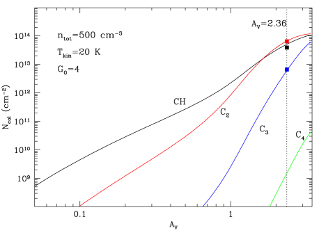
Figure 12: Abundances of CH, C₂, C₃, and C₄ carbon species computed as a function of the total visual absorption A_V.

It is a very complex task to make reasonable assumptions concerning the internal structure of any interstellar cloud. Clouds are likely non-homogeneous and asymmetrically irradiated by neighbouring stars. Another problem is the dust content. As demonstrated recently by Krełowski & Strobel (2012) the abundance ratio of the simple radicals CH and CN also depends on the shape of the extinction curve.

To illustrate the strong dependence on far-UV extinction we display spectra with very distinct C₂ spectral features toward two stars that have practically the same E(B-V). The data, shown in Fig. 13, are obtained from our present observation (HD 147165 in ESO Program 082.C-0566(A)) and from the ESO Archive (HD 210121 in Program 71.C-0513(C)). These spectra show that the C₂ abundance is drastically lower for the diffuse cloud toward HD 147165, which undergoes a low far–UV extinction field, than for the cloud towards HD 210121, which undergoes a high far–UV extinction field. The far-UV extinction curves can be found in Figs. 4.20 and 4.31 in the survey by Fitzpatrick & Massa (2007).

Figure 13: Spectral range of C₂ Phillips (2,0) band towards two objects HD 210121 and HD 147165 with similar colour excesses E(B-V) and different abundances of C₂.

8 Conclusion

We report on a high-quality absorption spectrum, in terms of both resolution and signal-to-noise ratio, of the C₃ molecule towards HD 169454. Besides a fully resolved spectrum of the à – X̃ 000 - 000 band at $\sim 4052$ Å seven further vibronic C₃ bands were identified in the range 3793-4000 Å. These absorptions had been suspected previously (Gausset et al., 1965), but now these bands are unambiguously detected for the first time with UVES-VLT. Four of those vibronic bands have been observed as well along the sight lines to two heavily reddened stars: HD 154368 and HD 73882. The observations are supported by laboratory measurements of all eight bands under high resolution using cavity ring-down laser spectroscopy.

The accurate value for the C₃ column density in the translucent cloud towards HD 169454 was included in an excitation model, applying the Meudon PDR-code by Roueff et al. (2002), yielding good agreement for the column densities of rotational levels. The calculations do not allow to determine gas density and destruction rate uniquely. As far as the rate coefficients and photodissociation rates are established, the model depends on the ratio of gas density to intensity of radiation field. When modifying the model with recently updated collisional rates (Ben Abdallah et al., 2008) the model results in high destruction rates required for C₃, inconsistent with the present understanding of the destruction process.

Observation of carbon chain molecules in optical spectra of diffuse clouds was up to now unsuccessful, except for C₃. All complex organic molecules identified in the interstellar space have been found in dense protostellar clouds. The detection and identification of a number of very weak absorptions of the C₃ molecule raises hope that the forest of narrow absorptions in the blue-violet part of the spectrum towards reddened stars may uncover assignments of heavier carbon species. Many weak as yet unidentified spectral features appear to be molecular lines, rather than noise. The regular pattern of C₃ bands allows for an unambiguous identification, as shown in the present study. Heavier species like C₄ and C₅ would produce more compact patterns due to the smaller rotational constant or due to a strong Q-branch compared to R- and P-branches characteristic for $\Sigma$–$\Pi$ transitions in case of C₅, particularly for low excitation temperature, which may lead to their detection. The assignment of absorption features in the UV-blue spectral range to the C₃ molecule is of relevance in the context of searches for carriers of the diffuse interstellar bands (DIBs). While most of the absorption features detected in translucent clouds in sight-lines toward reddened stars are ascribed to DIBs of unknown origin, the presently observed features can be excluded from the DIB-lists for which carriers are sought.

References

- Ádámkovics et al. (2003) Ádámkovics, M., Blake, G. A., & McCall, B. J. 2003, ApJ, 595, 235
- Balfour et al. (1994) Balfour, W. J., Ca, J., Prasad, C. V. V., & Qian, C. X. W., 1994, J. Chem. Phys., 101, 10343
- Becker et al. (1979) Becker, K. H., Tatarcyk, T., & Radić-Perić, J., 1979, Chem. Phys. Lett., 60, 502
- Ben Abdallah et al. (2008) Ben Abdallah, D., Hammami, K., Najar, F., Jaidane, N., Ben Lakhdar, Z., Senent, M. L., Chambaud, G., & Hochlaf, M., 2008, ApJ, 686, 379
- Casu & Cecchi-Pestellini (2012) Casu, S., & Cecchi-Pestellini, C., 2012, ApJ, 749, 48
- Cernicharo et al. (2000) Cernicharo, J., Goicochea, J. R., & Caux, E., 2000, ApJL, 534, 199
- Chabalowski et al. (1986) Chabalowski, C. F., Buenker, R. J., & Peyerimhoff, S. D., 1986, J. Chem. Phys., 84, 268
- Chen et al. (2010) Chen, C.-W., Merer, A., Chao, J.-W., & Hsu, Y.-C., 2010, J. Mol. Spec., 263, 56
- Clegg & Lambert (1982) Clegg, R. E. S., & Lambert, D. L., 1982, MNRAS, 201, 723
- Crawford (1997) Crawford, I. A., 1997, MNRAS, 290, 41
- Draine (1978) Draine, B. T., 1978, ApJS, 36, 595
- Fernie et al. (1983) Fernie, J. D., 1983, ApJS, 52, 7
- Douglas (1951) Douglas, A. E., 1951, ApJ, 114, 466
- Fitzpatrick & Massa (1990) Fitzpatrick E. L., Massa D., 1990, ApJS, 72, 163
- Fitzpatrick & Massa (2007) Fitzpatrick, E. L., & Massa, D., 2007, ApJ, 663, 320
- Galazutdinov (1992) Galazutdinov, G. A. 1992, Software publicly available via: http://gazinur.com/DECH-software.html
- Galazutdinov et al. (2002a) Galazutdinov, G., Pȩtlewski, A., Musaev, F., Moutou, C., Lo Curto, G., & Krełowski, J., 2002a, A&A, 395, 223
- Galazutdinov et al. (2002b) Galazutdinov, G., Pȩtlewski, A., Musaev, F., Moutou, C., Lo Curto, G., & Krełowski, J., 2002b, A&A, 395, 969
- Gausset et al. (1965) Gausset, L., Herzberg, G., Lagerqvist, A. & Rosen, B. 1965, ApJ, 142, 45
- Gendriesch et al. (2003) Gendriesch, R., Pehl, K., Giesen, T., Winnewisser, G., & Lewen, F., 2003, Z. Naturforsch. 58A, 129
- Giesen et al. (2001) Giesen, T. F., Van Orden, A. O., Cruzan, J. D., Provencal, R. A., Saykally, R. J., Gendriesch, R., Lewen, F., & Winnewisser, G., 2001, ApJL, 551, L181
- Haddad et al. (2014) Haddad, M. A., Zhao, D., Linnartz, H., & Ubachs, W. 2014, J. Mol. Spec., 297, 41
- Haffner & Meyer (1995) Haffner, L. M., & Meyer, D. M., 1995, ApJ, 453, 450
- Heger (1922) Heger, M. L., 1922, Lick. Obs. Bull. 10, 146
- Hinkle et al. (1988) Hinkle, K. W., Keady, J. J., & Bernath, P. F., 1988, Science, 241, 1319
- Hobbs et al. (2008) Hobbs, L. M., et al., 2008, ApJ, 680, 1256
- Hollenbach et al. (2009) Hollenbach, D., Kaufman, M. J., Bergin, E. A., & Melnick, G. J., 2009, ApJ, 690, 1497
- Huggins (1881) Huggins, W., 1881, Proc. R. Soc. London A, 33, 1
- Jannuzi et al. (1988) Jannuzi, B. T., Black, J. H., Lada, C. J., & van Dishoeck, E. F., 1988, ApJ, 332, 995
- Jongma et al. (1995) Jongma, R. T., Boogaarts, M. G. H., Holleman, I., & Meijer, G., 1995, Rev. Sci. Instrum., 66, 2821
- Jungen & Merer (1980) Jungen, C., & Merer, A. J., 1980, Mol. Phys., 40, 95
- Kazmierczak et al. (2010) Kazmierczak, M., Schmidt, M. R., Bondar, A. & Krełowski, J., 2010, MNRAS, 402, 2548
- Kazmierczak et al. (2010b) Kazmierczak, M., Schmidt, M. R., Galazutdinov, G.A., Betelesky, Y., & Krełowski, J., 2010, MNRAS, 408, 1590
- Kerr et al. (1998) Kerr, T. H., Hibbins, R. E., Fossey, S. J., Miles, J. R., & Sarre, P. J., 1998, ApJ, 495, 941
- Krełowski & Strobel (2012) Krełowski, J., & Strobel, A., 2012, Astron. Nachrichten, 333, 60
- Linnartz et al. (2000) Linnartz, H., Vizert, O., Motylewski, T., & Maier, J. P., 2000, J. Chem. Phys., 112, 9777
- Maier et al. (2001) Maier, J. P., Lakin, N. M., Walker, G. A. H., & Bohlender, D. A., 2001, ApJ, 553, 267
- (38) Maier, J. P., Walker, G. A. H., & Bohlender, D. A., 2002, ApJ, 566, 332
- (39) Maier, J. P., Walker, G. A. H., & Bohlender, D. A., 2004, ApJ, 602, 286
- McCall et al. (2003) McCall, B. J., Casaes, R. N., Ádámkovics, M., & Saykally, R. J., 2003, Chem. Phys. Lett., 374, 583
- Mendoza et al. (1958) Mendoza, V., E. E., 1958, ApJ, 128, 207
- Mookerjea et al. (2010) Mookerjea B., et al., 2010, A&A, 521, L13
- Mookerjea et al. (2012) Mookerjea, B., et al., 2012, A&A, 546, A75
- Motylewski & Linnartz (1999) Motylewski, T., & Linnartz, H., 1999, Rev. Sci. Instrum., 70, 1305
- Motylewski et al. (1999) Motylewski, T., Vaizert, O., Giesen, T. F., Linnartz, H., & Maier, J. P., 1999, J. Chem. Phys., 111, 6161
- Najar et al. (2008) Najar, F., Ben Abdallah, D., Jaidane, N., & Ben Lakhdar, Z., 2008 Chem. Phys. Lett, 460, 31
- Oka et al. (2003) Oka, T., Thorburn, J. A., McCall, B. J., Friedman, S. D., Hobbs, L. M., Sonnentrucker, P., Welty, D. E., & York D. G., 2003, ApJ, 582, 823
- Papaj et al. (1993) Papaj, J., Krełowski, J., & Wegner, W., 1993, A&A, 273, 575
- Le Petit et al. (2006) Le Petit, F., Nehmé, C., Le Bourlot, J., & Roueff, E., 2006, ApJS, 164, 506
- Radić-Perić et al. (1977) Radić-Perić, J., Roemelt, J., Peyerimhoff, S. D., & Buenker, R. J., 1977, Chem. Phys. Lett., 50, 344
- Roueff et al. (2002) Roueff, E., Felenbok, P., Black, J. H., & Gry, C., 2002, A&A, 384, 629
- Rousselot et al. (2001) Rousselot, P., Arpigny, C., Rauer, H., Cochran, A. L., Gredel, R., Cochran, W. D., Manfroid, J., & Fitzsimmons, A., 2001, A&A, 368, 689
- Sarre et al. (1995) Sarre, P. J., Miles, J. R., Kerr, T. H., Hibbins, R. E., Fossey, S. J., & Somerville, W. B., 1995, MNRAS, 277, L41
- Schmuttenmaer et al. (1990) Schmuttenmaer, C. A., Cohen, R.C., Pugliano, N., Heath, J. R., Cooksy, A. L., Busarow, K. L., & Saykally, R. J., 1990, Science, 249, 897
- Tanabashi et al. (2005) Tanabashi, A., Hirao, T., Amano, T., & Bernath, P. F., 2005, ApJ, 624, 1116
- Tokaryk & Chomiak (1997) Tokaryk, D. W., & Chomiak, D. E., 1997, J. Chem. Phys., 106, 7600
- van der Tak et al. (2007) van der Tak, F. F. S., Black, J. H., Schöier F. L., Jansen, D. J., & van Dishoeck, E. F., 2007, A&A, 468, 627
- van Dishoeck & Black (1982) van Dishoeck, E. F., & Black, J. H., 1982, ApJ, 258, 533
- van Dishoeck (1988) van Dishoeck E. F., 1988, ASSL, 146, 49
- Wegner (2002) Wegner W., 2002, BaltA, 11, 1
- Welty et al. (2013) Welty, D. E., Howk, J. C., Lehner, N., & Black, J. H., 2013, MNRAS, 428, 1107
- Weselak et al. (2004) Weselak, T., Galazutdinov, G. A., Musaev, F. A., & Krełowski J., 2004, A&A, 414, 949
- Woodall et al. (2007) Woodall, J., Agúndez, M., Markwick-Kemper, A. J., & Millar, T. J., 2007, A&A, 466, 1197
- Zhang et al. (2005) Zhang, G., Chen, K.-S., Merer, A. J., Hsu, Y.-C., Chen, W.-J., Shaji, S., & Liao, Y.-A., 2005, J. Chem. Phys. 122, 244308
- Zhao et al. (2011) Zhao, D., Haddad, M. A., Linnartz, H. L., & Ubachs, W., 2011, J. Chem. Phys., 135, 044307